An Adaptive Procedure for the Global Minimization of a Class of Polynomial Functions

Abstract

The paper deals with the problem of global minimization of a polynomial function expressed through the Frobenius norm of two-dimensional or three-dimensional matrices. An adaptive procedure is proposed which applies a Multistart algorithm according to a heuristic approach. The basic step of the procedure consists of splitting the runs of different initial points in segments of fixed length and to interlace the processing order of the various segments, discarding those which appear less promising. A priority queue is suggested to implement this strategy. Various parameters contribute to the handling of the queue, whose length shrinks during the computation, allowing a considerable saving of the computational time with respect to classical procedures. To verify the validity of the approach, a large experimentation has been performed on both nonnegatively constrained and unconstrained problems.

1. Introduction

Global optimization over continuous spaces is an important field of the modern scientific research and involves interesting aspects in computer science. Given an objective function f modeling a system of points which depends on a set of parameters, the task is to determine the set of parameters which optimizes f. For simplicity, in most cases the optimization problem is stated as a minimization problem.

For high dimensional problems, numerical methods are suggested which construct converging sequences of points by employing local optimizers, for example search methods. In general, procedures of this type are stochastic and rely on intensive computation to explore the solution space, without too deep enquires concerning convergence proofs. Roughly speaking, there are two main approaches: a sampling approach and an escaping approach. Examples of the sampling approach are Pure Random Search algorithms [1], where an extensive sampling of independent points is considered, and Multistart algorithms [2,3], which apply local optimizers to randomly generated starting points; then the best among the found local optima is considered the global optimum. Sampling algorithms have been shown [3] to converge in infinite time with probability 1, but in practice there is no guarantee that the best local solution found in a finite amount of computation is really the global optimum. In the escaping approach, various methods are devised for escaping from an already found local optimum, reaching other feasible points from which to restart a new local optimizer (see for example the Simulated Annealing [4]).

In practice, most algorithms succeed for small and medium-sized problems, but the chance of finding the global optimum worsens considerably when the number of the dimensions increases, due to the necessary limitation of the sampling set size. In any case, the computation of a local solution can be very expensive and the convergence of differently started local procedures to the same local optimum is frequent and should be avoided.

In this paper we propose an adaptive strategy for finding the global minimum of a polynomial function expressed through the Frobenius norm of matrices and tensors. The considered problem is outlined in Section 2. The Multistart algorithm, on which the adaptive strategy is based, is described in Section 3. It implements a particularly tailored local minimization procedure with an ad-hoc stopping condition. The basic step of the adaptive strategy is implemented through a priority queue and consists in splitting the runs starting from different initial points in segments of fixed length. The processing order of the various segments is interlaced, discarding those which appear less promising. The adaptive procedure is described in Section 4. Finally, in Section 5 the validity of the adaptive procedure is verified through a large experimentation on both nonnegatively constrained and unconstrained problems.

2. The Problem

A widely studied problem in literature is the one of nonlinear global minimization

$$\underset{\mathit{x}\in D}{\min }f\left(\mathit{x}\right),$$

(1)

where $D\subseteq {\mathbb{R}}^N$ is a region determined by a set of constraints and $f:D\to {\mathbb{R}}_{+}$ is a polynomial function of degree $d\ge 2$ which models the problem’s objective. Classical examples are $D={\mathbb{R}}_{+}^N$ of nonnegativity constraints, and $D={\mathbb{R}}^N$ when no constraint is given. Problem (1) is NP-hard [5]. In this paper we consider specifically objective functions expressed through the Frobenius norm of an array $\mathcal{A}$ whose elements are low degree polynomials in the entries of $\mathit{x}$:

$$f\left(\mathit{x}\right)={\parallel \mathcal{A}\left(\mathit{x}\right)\parallel }_F^2.$$

(2)

We examine in particular the cases where $\mathcal{A}\left(\mathit{x}\right)$ is a two-dimensional or a three-dimensional matrix. For example, in the two dimensional case, a problem considered in the experimentation looks for two low-rank matrices $W\in {\mathbb{R}}_{+}^{m\times k}$ and $H\in {\mathbb{R}}_{+}^{n\times k}$ such that $M\approx W{H}^T$ according to

$$\underset{W,H\ge O}{\min }f(W,H),\mathrm{where}f(W,H)={\parallel M-W{H}^T\parallel }_F^2,$$

(3)

given a nonnegative matrix $M\in {\mathbb{R}}_{+}^{m\times n}$ and an integer $k<n$. Problem (3), known as Nonnegative Matrix Factorization (NMF), was first proposed in [6] for data analysis and from then on has received much attention. It is a particular case of Problem (1) with $f\left(\mathit{x}\right)$ as in (2), $N=(m+n)k$, $D={\mathbb{R}}_{+}^N$ and $\mathit{x}$ a vectorization of the pair $(W,H)$. In a columnwise vectorization, $\mathcal{A}\left(\mathit{x}\right)$ is the matrix of elements

$$a_{i,j}\left(\mathit{x}\right)=m_{i,j}-\sum _{r=1}^k{w}_{i,r}{h}_{j,r}=m_{i,j}-\sum _{r=1}^k{x}_{(r-1)m+i}{x}_{mk+(r-1)n+j}.$$

Since f is a polynomial, the gradient $\nabla f$ and the Hessian ${\nabla }^{2}f$ of f are available. From a theoretical point of view, a simple way to solve Problem (1) in the unconstrained case would be to look for the stationary points $\mathit{x}$ where $\nabla f\left(\mathit{x}\right)=0$ and choose whichever $\mathit{x}$ minimizes f, but this way does not appear to be practical when N is large, even if d is not too large, because finding a global minimum can be a very difficult task when f has many local minima. For this reason, numerical methods have been proposed which do not try to solve $\nabla f\left(\mathit{x}\right)=0$. Anyway, many numerical methods take advantage of derivative information to improve the computation.

When the dimension N is very large, also numerical methods which require at the same time $O\left(N\right)$ active points might be impracticable. This is the case, for example, of methods such as Nelder–Mead algorithm [7] which works on a polytope of $N+1$ vertices, or Differential Evolution [8] which generates at each iteration a new population of more than $N+1$ points, or Simulated Annealing [9] which for the continuous minimization uses a downhill simplex of $N+1$ points. In this paper we propose a method which allows solving Problem (1) also when N is very large. To validate its performances against other methods, it is necessary to restrict our experimentation to dimensions where the other methods could still compute reliable solutions.

3. A Multistart Algorithm

Multistart algorithms are widely used heuristics for solving Problem (1) [2,3]. Over the years, many variants and generalizations have been produced. We consider here its basic form which consists of the following steps:

• start with a fixed number q of independent initial points ${\mathit{x}}_0^{\left(r\right)}$, $r=1,\dots ,q$, randomly generated.
• For $r=1,\dots ,q$, a local optimizer, say $\mathcal{L}$, is applied to ${\mathit{x}}_0^{\left(r\right)}$ to find an approximation of a local minimum. We assume $\mathcal{L}$ to be an iterative procedure which, in the constrained case, takes on the nonnegativity of $\mathit{x}$ and denote by ${\mathit{x}}_{\nu }^{\left(r\right)}$, $\nu =1,2,\dots$, the sequence of points computed until a suitable stopping condition is satisfied. The corresponding function values $f({\mathit{x}}_{\nu }^{\left(r\right)})$ estimate the quality of the approximation. Both the chosen procedure $\mathcal{L}$ and the stopping condition employed by $\mathcal{L}$ are of crucial importance. Ideally, the stopping condition should verify whether the local minimum has been reached within a given tolerance $ϵ$, but of course more practical tests must be used.
• When all the q points ${\mathit{x}}_0^{\left(r\right)}$ have been processed, the point ${\mathit{x}}_{\nu }^{\left(r\right)}$ with the smallest function value $f({\mathit{x}}_{\nu }^{\left(r\right)})$ is selected as an approximation of the global minimum. It is evident that the minimum found in this way is not guaranteed to suitably approximate the global minimum, even if a large number of starting points is considered.

In the experimentation we have implemented a version of the basic Multistart algorithm, here denoted by MS, as reference. The chosen local optimizer $\mathcal{L}$ is particularly suitable for the problems we are considering and exploits the differentiability of the function $f\left(\mathit{x}\right)$. Its execution time turns out to be much smaller than what is generally expected from a library method, which relies on general purpose procedures as local optimizers and does not exploit the differentiability information. The stopping condition we have implemented monitors the flatness of the approximation by assuming ${\mathit{x}}_{\nu }^{\left(r\right)}$ as an acceptable approximation of a local minimum when

$$(\max \mathit{g}-\min \mathit{g})/\mathrm{mean}\mathit{g}\le ϵ,\mathrm{where}\mathit{g}=[f({\mathit{x}}_{\nu -2}^{\left(r\right)}),f({\mathit{x}}_{\nu -1}^{\left(r\right)}),f({\mathit{x}}_{\nu }^{\left(r\right)})].$$

(4)

Of course, if an index $\nu$ exists such that $f({\mathit{x}}_{\nu }^{\left(r\right)})=0$, the algorithm stops and condition (4) is not tested. The tolerance $ϵ$ is set equal to some power of the machine $eps$. As usual, a maximum number $d_{\max }$ of allowed iterations is imposed to each run.

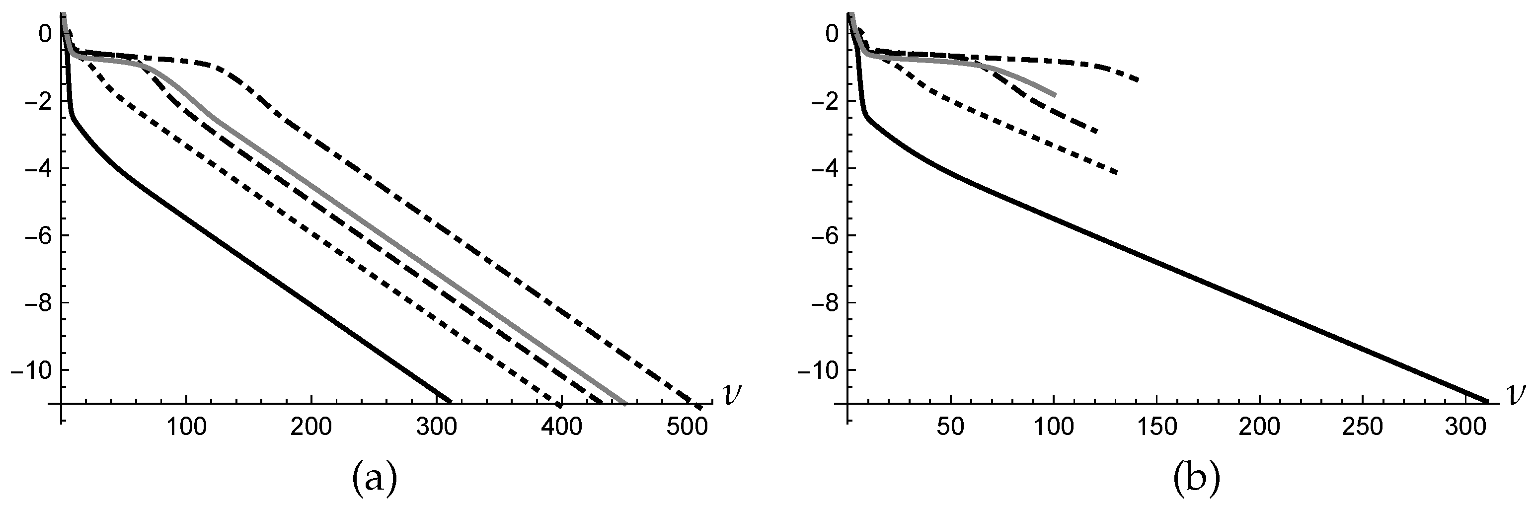
As an example, we have applied MS to one of the problems described in Section 5.3, namely problem $10\times 5\times 15(5,3)$, generating $q=5$ initial points. Figure 1a shows the log plot of the histories $f({\mathit{x}}_{\nu }^{\left(r\right)})$, $\nu =1,2,\dots$, computed by MS for $r=1,\dots ,q$ using the stopping condition (4) with $ϵ={10}^{-12}$. All the sequences converge to the same local minimum, but one (plotted with black solid line) requires 300 iterations and appears to be faster than the others which require from 400 to 500 iterations. The number of iterations of the overall execution is 2100.

Figure 1. (a) History plots of MS; (b) History plots of AD.

Letting the local algorithm run until convergence for all the starting points is a time-consuming procedure, in particular when the iterates obtained from many different starting points lead to the same local minimum. A reasonable approach, that we presently propose, modifies this procedure adaptively. It is based on an efficient premature recognition of the more promising runs of the local algorithm and interrupts with high probability the runs which may lead to already found local minima or to local minima of larger value than those already found.

4. An Adaptive Procedure

Because of the large computational cost of the strategy described in the previous section, the straightforward implementation can be profitably applied only to small problems. For this reason we propose here a heuristic approach, which we denote by the name AD, suitable for large problems whose basic step consists in the splitting of the runs in segments of a fixed length $\lambda$. Each segment, identified by the index r, $r=1,\dots ,q$, stores the partial solution produced at the end of the $\lambda$ iterations, which will be used as the starting point for the next run with the same index r. The processing order of the various segments is modified by interlacing the computation of segments with different indices r. This strategy requires segments corresponding to different r’s to be available at any moment of the computation. The segments, which appear to be the more promising ones depending on the behavior of the computed function values, are carried on and the other segments are discarded.

The strategy is accomplished using a priority queue $\mathcal{Q}$ whose items have the form

$$Y=\{r,h,\mathit{x},\mathit{g},\delta ,\chi \},r=1,\dots ,q,$$

where

• $r\in \{1,\dots ,q\}$ is the index of the segment; it identifies the seed chosen for the random generation of the initial point following a uniform distribution between 0 and 1.
• $h=h^{\left(r\right)}$ is the number of iterations computed until now by $\mathcal{L}$ in all the segments with the same index r, i.e., starting with ${\mathit{x}}_0^{\left(r\right)}$.
• $\mathit{x}={\mathit{x}}_h^{\left(r\right)}$ is the partial solution computed by $\mathcal{L}$ at the end of the current rth segment.
• $\mathit{g}=[f({\mathit{x}}_{h-2}^{\left(r\right)}),f({\mathit{x}}_{h-1}^{\left(r\right)}),f({\mathit{x}}_h^{\left(r\right)})]$ is the array containing the function values of the last three points computed by $\mathcal{L}$ in the current rth segment.
• $\delta =f({\mathit{x}}_{h-1}^{\left(r\right)})-f({\mathit{x}}_h^{\left(r\right)})$ is an estimate of the decreasing rate of the function.
• $\chi ={\chi }^{\left(r\right)}$ is the priority of the item, which rules the processing order of the various segments according to the minimum policy.

The belonging of an element to an item Y is denoted by using the subscript $\left(Y\right)$, for example $r_{\left(Y\right)}$ denotes the index of item Y.

During the computation three global quantities, $g_{\min }$, ${\mathit{x}}_{\min }$, and $r_{\min }$, play an important role:

• $g_{\min }$ is the minimum of all the function values computed so far relative to all the items already processed
• ${\mathit{x}}_{\min }$ is the computed point corresponding to $g_{\min }$ and $r_{\min }$ is the index of the item where $g_{\min }$ has been found.

The priority is defined by $\chi =\gamma +\xi$, where $\gamma ={\log }_{10}(f\left(\mathit{x}\right)/g_{\min })$ measures the accuracy of the last computed iterate in the current segment and $\xi =h/\lambda$ measures the age of the computation of the rth seed. Between two items which have the same age, this expression favors the one with the better accuracy and, between two items which have comparable accuracies, it favors the younger one, that is the quicker one. The inclusion of the age into the priority is important to avoid that only the best item is processed and all the other items are ignored. In fact, with the increase of the age, also items which had been left behind take their turn.

At the beginning the initial points ${\mathit{x}}_0^{\left(r\right)}$, $r=1,\dots ,q$, are randomly generated and $g_{\min }={\min }_{r=1,\dots ,q}f({\mathit{x}}_0^{\left(r\right)})$ is set. The initial priorities are defined by ${\chi }^{\left(r\right)}={\log }_{10}(f({\mathit{x}}_0^{\left(r\right)})/g_{\min })$ and the queue is formed by the q items

$$\{r,h,{\mathit{x}}_0^{\left(r\right)},\mathit{g},\delta ,{\chi }^{\left(r\right)}\},\mathrm{for}r=1,\dots ,q,$$

(5)

where $h=\delta =0$ and $\mathit{g}$ is a void array.

The length of the queue, i.e., the number of items in $\mathcal{Q}$, is found by calling the function Length. At the beginning the length is q and it is modified by the functions:

• Y = Dequeue $\left(\mathcal{Q}\right)$ returns the item Y which has the smallest priority and deletes it from $\mathcal{Q}$,
• Enqueue$(\mathcal{Q},Y)$ inserts the item Y into $\mathcal{Q}$.

A further function Maxdelta $\left(\mathcal{Q}\right)$ returns the largest value among the quantities $\delta$ of all the items in $\mathcal{Q}$.

During the computation the following quantities deriving from $\mathit{g}={\mathit{g}}_{\left(Y\right)}$, $h=h_{\left(Y\right)}$ and $\delta ={\delta }_{\left(Y\right)}$ are referred (their expressions have been tested by an ad hoc experimentation):

• $\vartheta =(\max \mathit{g}-\min \mathit{g})/\mathrm{mean}\mathit{g}$ measures the flatness of the last computed values of f according to (4),
• $\phi =\delta /\mathrm{mean}\mathit{g}$ measures the decreasing rate of f. If $\phi <0$ the last computed iteration increases over the preceding one. Only small increases, corresponding to limited oscillations, are tolerated,
• $c={(1-2^{-\xi /\lambda })}^2+0.5(f\left(\mathit{x}\right)-g_{\min })/f\left(\mathit{x}\right)$ measures the discarding level. The larger c, the higher the probability of discarding the item. Among items which have comparable values $f\left(\mathit{x}\right)$, the older one has greater probability to be discarded.

Three other functions are needed:

• Random$\left(n\right)$ generates n numbers uniformly distributed over $[0,1]$.
• The local minimization algorithm $\mathcal{L}$ is applied for the predefined number $\lambda$ of iterations (in the experiments we assume $\lambda =10$) and returns $\mathit{x}$, $\mathit{g}$, the minimum $\widehat{g}$ of the function values of the current segment, its corresponding point $\widehat{\mathit{x}}$, the number $\nu$ of performed iterations and the decreasing rate $\delta$. Since algorithm AD is based on the splitting into segments of the run corresponding to a single starting point, the local optimizer $\mathcal{L}$ needs to be stationary, in order to get a computation which gives the same numerical values as if a single run had been performed without segmentation.
• The following Boolean function Control verifies whether an item is promising (i.e., must be further processed) or not. For notes (a)–(e) see the text.

Function Control$\left(Y\right)$;

the selected item Y is enqueued again if True is returned, otherwise it is discarded.

$\mathit{g}={\mathit{g}}_{\left(Y\right)}$;   $h=h_{\left(Y\right)}$;   $\delta ={\delta }_{\left(Y\right)}$;   compute $\vartheta$, $\phi$ and c;

if $\phi <-0.6$ then return False;   (a)

if $\vartheta <ϵ$, then return False;   (b)

if Length $\left(\mathcal{Q}\right)>2$ and $\delta \ge$ Maxdelta$\left(\mathcal{Q}\right)$ then return True;   (c)

if $r_{\left(Y\right)}=r_{\min }$, then return True;   (d)

if Random $\left(1\right)<c$ then return False;   (e)

return True;

The decision on which course to choose depends mainly on the flatness, but other conditions are also taken into consideration as described in the following notes:

(a)

large oscillations are not allowed,

(b)

the flatness level has been reached,

(c)

the selected item decreases more quickly than other items in the queue,

(d)

the selected item has the same index r of the item where $g_{\min }$ has been found,

(e)

if none of the preceding conditions holds, the selected item is discarded with probability given by its discarding level.

After the initialization of the queue, the adaptive process AD evolves as follows: an item Y is extracted from the queue according to its priority ${\chi }_{\left(Y\right)}$. When enough iterations ($6\lambda$ iterations in the experiments) have been performed for stabilizing the initial situation, the function Control is applied, and if Y is recognized promising, the function $\mathcal{L}$ is applied to point ${\mathit{x}}_{\left(Y\right)}$. A new item is so built and inserted back into $\mathcal{Q}$. If the computed $f\left(\widehat{\mathit{x}}\right)$ is smaller than $g_{\min }$, then $g_{\min }$, ${\mathit{x}}_{\min }$ and $r_{\min }$ are updated. Otherwise, if Y is not promising, no new item is inserted back into $\mathcal{Q}$, i.e., Y is discarded. At the end, ${\mathit{x}}_{\min }$ and $f\left({\mathit{x}}_{\min }\right)$ are returned. A bound $d_{\max }$ is imposed on the number of iterations of the overall execution.

Our proposed algorithm is implemented in the following function Chi.

function Chi$\left(q,\lambda ,ϵ,d_{\max }\right)$;

for $r=1,\dots ,q$ let ${\mathit{x}}_0^{\left(r\right)}=$ Random (N);

initialize $r_{\min },{\mathit{x}}_{\min },g_{\min },$;   initialize $\mathcal{Q}$ according to (5);

$d=0$;

while Length $\left(\mathcal{Q}\right)\ge 1$ and $g_{\min }>ϵ$ and $d<d_{\max }$

Y = Dequeue $\left(\mathcal{Q}\right)$;

$cond=$ True;

if $h_{\left(Y\right)}>6\lambda$ then cond = Control (Y);

if cond then

$(\mathit{x},\mathit{g},\widehat{g},\widehat{\mathit{x}},\nu ,\delta )=\mathcal{L}({\mathit{x}}_{\left(Y\right)},\lambda )$;

d = d + ν;   h = hY + ν;    χ = log10(f(x)/gmin)+h/λ;

Enqueue ($\mathcal{Q}$,{r(Y),h,x,g,δ,χ});

if $\widehat{g}$ < gmin then gmin = $\widehat{g}$; xmin = $\widehat{\mathit{x}}$; rmin = r(Y);

end if

end while

returnxmin and f(xmin);

Figure 1b shows the log plots of the histories $f({\mathit{x}}_{\nu }^{\left(r\right)})$ obtained by applying AD to the same problem of the example considered in Section 3 with MS, using also the same $q=5$ initial points. Only the sequence plotted with the black solid line survives in the queue, while all the other sequences are discarded from the queue at different steps of the computation. At the end 800 overall iterations have been performed, compared with the 2100 of MS, as it is evident from the two figures, pointing out the outperformance of AD on MS.

5. Experimentation

The experimentation is performed with a 3.2 GHz 8-core Intel Xeon W processor machine using IEEE 754-64 bit double precision floating point format (with $eps=2.22\times {10}^{-16}$) and is carried out on the three nonnegatively constrained test problems described in Section 5.1, Section 5.2 and Section 5.3 and on the unconstrained test problem described in Section 5.4. The following methods are applied to each test problem.

• Class 1 methods: library versions of Nelder–Mead method (denoted in the tables by the name NM), Differential Evolution (denoted DE) and Simulated Annealing (denoted SA). These methods are run for at most 200 iterations and are applied for comparison purpose.
• Class 2 methods: the Multistart procedure described in Section 3 (denoted MS) and the adaptive procedure described in Section 4 (denoted AD). Two values for the tolerance $ϵ$ in (4) are used by MS and AD, namely ${ϵ}_1={10}^{-8}\sim ep{s}^{1/2}$ and ${ϵ}_2={10}^{-12}\sim ep{s}^{3/4}$. The names MS1 and AD1 refer to ${ϵ}_1$ and the names MS2 and AD2 refer to ${ϵ}_2$. The number of randomly generated initial points is $q=10$. The bound to the number of iterations for each run of MS is $d_{\max }=1000$, while the overall number of iterations of AD is bounded by $d_{\max }=5000$.

With Class 2 methods the procedure $\mathcal{L}$ used as local minimizer differs according to the presence of constraints or not. In the test problems two different situations occur:

• The problem has a region D related to nonnegativity constraints. In this case, a block nonlinear Gauss–Seidel scheme [10] is implemented as $\mathcal{L}$, in order to find constrained local minima of $f\left(\mathit{x}\right)$. The vector $\mathit{x}$ is decomposed into $\mu$ disjoint subvectors, cyclically updated until some convergent criterium is satisfied. The convergence of this scheme, more specifically called in our case Alternating Nonnegative Least Squares (ANLS), is analyzed in [10]. We apply it for the particular case of Problem (1) with $f\left(\mathit{x}\right)$ as in (2) in the two-dimensional case ($\mu =2$ in Section 5.1 and Section 5.2) and in the three-dimensional case ($\mu =3$ in Section 5.3).
• The problem is unconstrained (Section 5.4). In this case the local minimizer $\mathcal{L}$ is a library procedure based on Levenberg-Marquardt method.

The aim of the experimentation is:

• To analyze, in terms of both execution time and accuracy, the effects on the performance of Class 2 methods of the two chosen values for the tolerance $ϵ$ used in the stopping condition (4). Of course, we expect that a weaker request for the tolerance (${ϵ}_1={10}^{-8}$) would result in lower accuracy and time saving than a stronger request (${ϵ}_2={10}^{-12}$). This issue is experimentally analyzed by comparing the performances of method MS1 with those of method MS2 and the performances of method AD1 with those of method AD2.
• To compare the performances of the adaptive and non adaptive procedures of Class 2. We wonder whether the adaptive procedure, with its policy of discarding the less promising items, can overlook the item which eventually would turn out to be the best one. This issue is experimentally analyzed by comparing the performances of method MS1 with those of method AD1 and the performances of method MS2 with those of method AD2.
• To compare the performances of Class 1 and of Class 2 methods. Naturally, we expect that in the case of constrained problems the execution times of Class 1 methods, which implement general purpose procedures, would be larger than those of Class 2, specifically tailored to functions of type (2). Beforehand, it is not clear whether the latter ones would pay the time saving with a lower accuracy.

For each problem we assume that an accurate approximation of the solution $f^{*}$ of (1) is known. In the tables two performance indices are listed:

• the execution time (denoted $time$) in seconds. In order to get a more reliable measure for this index, the same problem is run 5 times with each starting point and the average of the measures is given in the tables as $time$.
• the quantity $lerr=-{\log }_{10}(f\left({\mathit{x}}_{\min }\right)-f^{*})$, rounded to the first decimal digit, as a measure of accuracy. Approximately, $lerr$ gives the number of exact decimal digits obtained by the method. The larger $lerr$, the more accurate the method. When a method produces a very good value $f\left({\mathit{x}}_{\min }\right)$ such that $f\left({\mathit{x}}_{\min }\right)-f^{*}\sim eps$, the case is marked by the symbol +.

We give now a description of the test problems together with their numerical results.

5.1. The Nonnegative Matrix Factorization

The first test problem is the NMF problem (3) already outlined in Section 2, i.e., given $M\in {\mathbb{R}}_{+}^{m\times n}$ and $k<n$, we look for the basis matrix $W\in {\mathbb{R}}_{+}^{m\times k}$ and the coefficient matrix $H\in {\mathbb{R}}_{+}^{n\times k}$ which minimize $f(W,H)=\parallel M-W{H}^T{\parallel }_F^2$ under the constrains $W,H\ge O$.

ANLS is applied to $f(W,H)$ with $\mu =2$. An initial $W_0\in {\mathbb{R}}_{+}^{m\times k}$ is chosen and the sequences

$$\left\{\begin{array}{c}{H}_{\nu }=\underset{H\ge 0}{\mathrm{argmin}}{\parallel M-W_{\nu -1}{H}^T\parallel }_F^2,\hfill \\ W_{\nu }=\underset{W\ge 0}{\mathrm{argmin}}{\parallel M^T-H_{\nu }{W}^T\parallel }_F^2,\hfill \end{array}\right.$$

(6)

for $\nu =1,2,\dots$, are computed.

Although the original problem (3) is nonconvex, subproblems (6) are convex and can be easily dealt with. In the experimentation we use for (6) the Greedy Coordinate Descent method (called GCD in [11]), which is specifically designed for solving nonnegative constrained least squares problems. The attribute “Greedy” refers to the selection policy of the elements updated during the iteration, based on the largest decrease of the objective function. In our tests this method has shown to be fast and reliable. The corresponding code can be found as Algorithm 1 in [11].

For the experimentation, given the integers m, n and $h\le \min \{m,n\}$, two matrices $A\in {\mathbb{R}}_{+}^{m\times h}$ and $B\in {\mathbb{R}}^{n\times h}$ are generated with random elements uniformly distributed over $[0,1]$ and the matrix $M=A{B}^T$ is constructed. The test problem (3) requires computing the NMF of M, i.e., given an integer $k\le h$, two matrices $W\in {\mathbb{R}}_{+}^{m\times k}$ and $H\in {\mathbb{R}}_{+}^{n\times k}$ such that $M\approx W{H}^T$ are to be found. The following cases are considered

$$\begin{array}{c}m=20,n=10,h=5,\mathrm{with}k=3\mathrm{and}k=5,\hfill \\ m=40,n=30,h=10,\mathrm{with}k=5\mathrm{and}k=10.\hfill \end{array}$$

The dimension of the solution space is $N=(m+n)k.$ In the cases $k=h$ we expect $f^{*}=0$. The results are shown in Table 1.

Table 1. Execution times and accuracies for nonsymmetric Nonnegative Matrix Factorization (NMF) problems.

m × n (h, k)	N	Indices	NM	DE	SA	MS1	MS2	AD1	AD2
$20\times 10(5,3)$	90	$time$	18	42	38	19	27	16	18
		$lerr$	14.1	13.7	13.4	12.9	13.	12.9	13.0
$20\times 10(5,5)$	150	$time$	336	168	536	37	55	7	8
		$lerr$	13.9	13.2	13.6	8.9	+	8.2	+
$40\times 30(10,5)$	350	$time$	617	696	783	200	323	135	148
		$lerr$	12.1	12.4	12.5	6.6	10.8	6.6	10.8
$40\times 30(10,10)$	700	$time$	3158	5011	3929	606	917	183	255
		$lerr$	13.2	11.5	12.2	8.6	12.4	8.6	12.0

In the table we note that Class 1 methods, which use general purpose local optimizers, are more time consuming than Class 2 methods, as expected. Moreover, this gap increases with the dimension N. Averagely, Class 1 methods are more accurate than Class 2 methods. Within the Class 2, each adaptive method is faster than the corresponding non adaptive one, as can be seen by comparing the times in column AD1 with those in column MS1 and the times in column AD2 with those in column MS2. Obviously, MS1 and AD1 give lower accuracies than MS2 and AD2 respectively, due to a weaker request on the flatness imposed by (4). By comparing the measures $lerr$ in column AD2 with those in column MS2, we see that AD2 does not lose accuracy with respect to MS2.

5.2. The Symmetric NMF

In some applications, matrix $M\in {\mathbb{R}}_{+}^{n\times n}$ is symmetric, then the objective function to be minimized becomes $f\left(W\right)=\parallel M-W{W}^T{\parallel }_F^2$, under the constrain $W\ge O$. This problem is known as symmetric NMF (SymNMF). As suggested in [12], the solution $W\in {\mathbb{R}}_{+}^{n\times k}$ can be found through a nonsymmetric penalty problem of the form

$$\underset{W,H\ge O}{\min }{f}_{\alpha }(W,H),\mathrm{with}{f}_{\alpha }(W,H)=\parallel M-W{H}^T{\parallel }_F^2+\alpha {\parallel W-H\parallel }_F^2,$$

$\alpha$ being a positive parameter which acts on the violation of the symmetry. Hence, applying ANLS, we solve alternatively the two subproblems

$$H_{\nu }=\underset{H\ge 0}{\mathrm{argmin}}{\parallel \left[\begin{array}{c}M\\ \sqrt{{\alpha }_{\nu }}{W}_{\nu -1}^T\end{array}\right]-\left[\begin{array}{c}{W}_{\nu -1}\\ \sqrt{{\alpha }_{\nu }}{I}_k\end{array}\right]H^T\parallel }_F^2,$$

$$W_{\nu }=\underset{W\ge 0}{\mathrm{argmin}}{\parallel \left[\begin{array}{c}M\\ \sqrt{{\alpha }_{\nu }}{H}_{\nu }^T\end{array}\right]-\left[\begin{array}{c}{H}_{\nu }\\ \sqrt{{\alpha }_{\nu }}{I}_k\end{array}\right]W^T\parallel }_F^2.$$

In [12], the sequence of penalizing parameters is constructed by setting

$${\alpha }_{\nu }={\beta }_{\nu }\max M,\mathrm{with}{\beta }_0=1$$

and ${\beta }_{\nu }$ is modified according to a geometric progression of the form ${\beta }_{\nu }={\zeta }^{\nu }$ with the fixed ratio $\zeta =1.01$. We suggest instead to let ${\beta }_{\nu }$ be modified adaptively, as shown in [13].

Symmetric NMF problems arise naturally in clustering. Given n points ${\mathit{p}}_i$ in an Euclidean space and the number k of the required clusters, the clustering structure is captured by a symmetric matrix M, called similarity matrix, whose elements $m_{i,j}$ represent the similarity between ${\mathit{p}}_i$ and ${\mathit{p}}_j$. These similarity values are computed through the Gaussian kernel

$$e_{i,j}=\exp \left(-\frac{\parallel {\mathbf{p}}_i-{\mathbf{p}}_j{\parallel }_2^2}{{\sigma }^2}\right),\mathrm{for}i\ne j,\mathrm{and}{e}_{i,i}=0,$$

(7)

where $\sigma$ is a suitable scaling parameter, followed by the normalized cut

$$m_{i,j}=d_i^{-1/2}{e}_{i,j}{d}_j^{-1/2}\mathrm{where}{d}_i=\sum _{r=1}^n{e}_{i,r},\mathrm{for}i=1,\dots ,n.$$

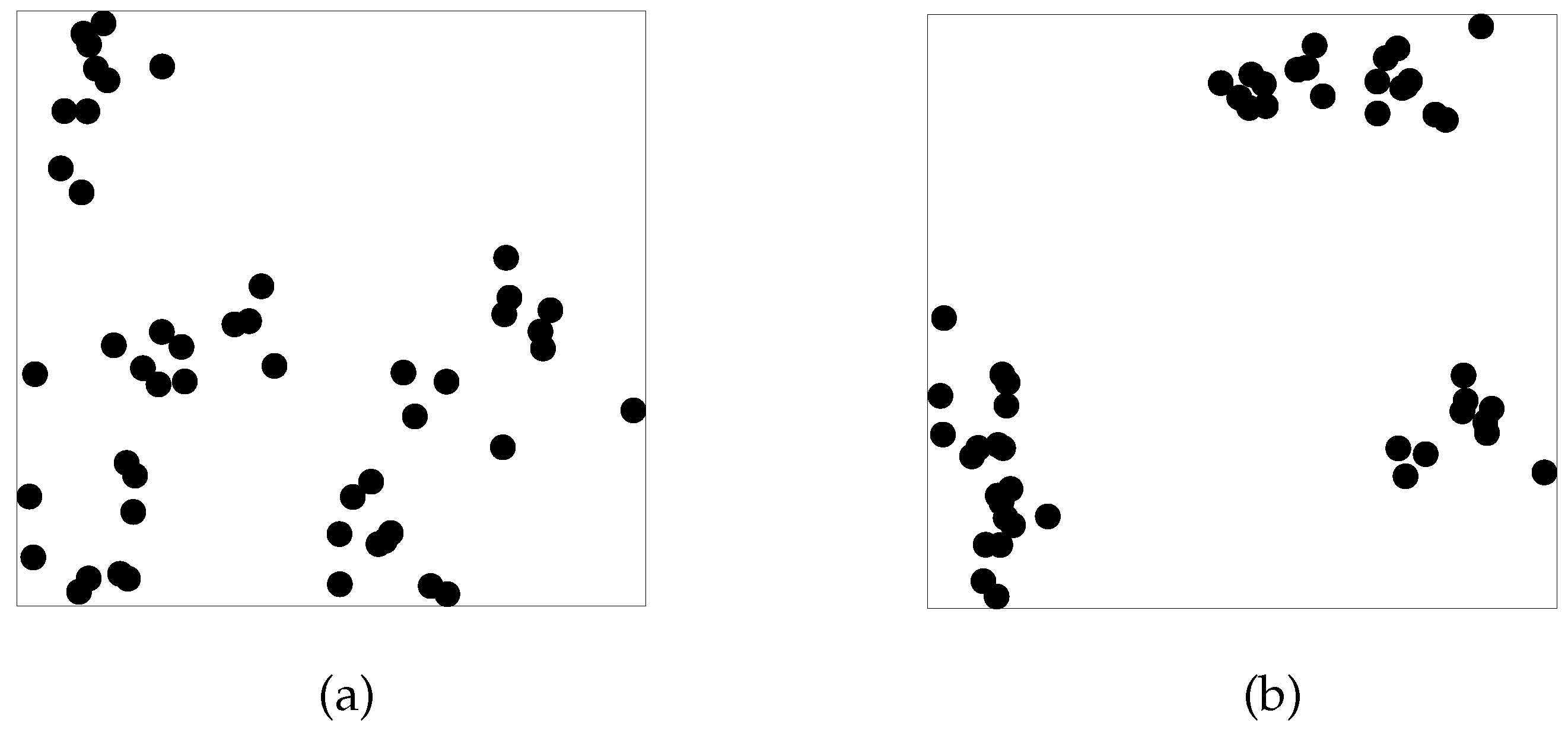
The experimentation deals with two sets $C_1$ and $C_2$ of n points randomly generated in ${\mathbb{R}}^2$ (see Figure 2 for $n=50$).

Figure 2. (a) Set $C_1$ and (b) Set $C_2$ with $n=50$ points.

Set $C_1$ is generated with $n=10,50,100$ and set $C_2$ is generated with $n=50,100,200.$ The number of the required clusters is fixed to $k=5$ for all the cases. The dimension of the solution space is $N=2nk.$ The results are shown in Table 2. On these problems, Class 2 methods outperform Class 1 methods in both the computational time and the accuracy. Moreover, by comparing the measures $lerr$ in column AD1 with those in column MS1 and the measures $lerr$ in column AD2 with those in column MS2, we see that, for each value of the tolerance $ϵ$, the adaptive method and the corresponding non adaptive one share the same accuracy.

Table 2. Execution times and accuracies for symmetric Nonnegative Matrix Factorization (NMF) problems.

cluster	N	Indices	NM	DE	SA	MS1	MS2	AD1	AD2
$C_1,n=10$	100	$time$	5	18	11	10	10	6	6
		$lerr$	+	+	+	+	+	+	+
$C_1,n=50$	500	$ltime$	1232	1092	1363	15	14	12	13
		$err$	8.6	8.6	8.6	+	+	+	+
$C_2,n=50$	500	$time$	991	1138	1085	12	12	11	11
		$lerr$	8.5	8.5	8.5	+	+	+	+
$C_1,n=100$	1000	$time$	7541	8275	7749	108	107	83	87
		$lerr$	8.2	8.3	8.2	+	+	+	+
$C_2,n=100$	1000	$time$	5577	5645	6184	84	94	81	82
		$lerr$	8.6	8.6	8.6	14.8	14.8	14.8	14.8
$C_2,n=200$	2000	$time$	28,003	36,256	37,424	356	421	137	164
		$lerr$	9.2	9.8	9.8	9.0	+	9.0	+

5.3. The Nonnegative Factorization of a 3rd-Order Tensor

Let T be a 3rd-order tensor, i.e., a three-dimensional array whose elements are $t_{i,j,k}$, with $i=1,\dots ,m$, $j=1,\dots ,n$ and $k=1,\dots ,\ell$. A common way to represent graphically T is through its (frontal) slices $T_k$, $k=1,\dots ,\ell$, where $T_k$ is the matrix obtained by fixing to k the third index.

If T can be expressed as the outer product of three vectors $\mathit{u}$, $\mathit{v}$ and $\mathit{z}$, i.e., $T=\mathit{u}\circ \mathit{v}\circ \mathit{z}$, where ∘ denotes the vector outer product, T is called rank-one tensor or triad.

Among the many factorizations of a tensor defined in the literature, we consider here the CANDECOMP/PARAFAC (in the following CP) decomposition (see [14]) into the sum of triads, which extends in a natural way the decomposition of matrices in sum of dyads. Given an integer $\rho$, three matrices $U\in {\mathbb{R}}^{m\times \rho }$, $V\in {\mathbb{R}}^{n\times \rho }$ and $Z\in {\mathbb{R}}^{\ell \times \rho }$ are computed such that

$$T\approx \sum _{s=1}^{\rho }{\mathit{u}}_s\circ {\mathit{v}}_s\circ {\mathit{z}}_s,$$

(8)

where ${\mathit{u}}_s$, ${\mathit{v}}_s$ and ${\mathit{z}}_s$ are the sth columns of U, V and Z (see [14,15]). Elementwise, (8) is written as

$$t_{i,j,k}\approx \sum _{s=1}^{\rho }{u}_{i,s}{v}_{j,s}{z}_{k,s},\mathrm{for}i=1,\dots ,m,j=1,\dots ,n,k=1,\dots ,\ell .$$

The objective function of the CP decomposition of T is

$${\displaystyle f(U,V,Z)=\parallel T-\sum _{s=1}^{\rho }{\mathit{u}}_s\circ {\mathit{v}}_s\circ {\mathit{z}}_s{\parallel }_F^2=\sum _{i=1}^m\sum _{j=1}^n\sum _{k=1}^{\ell }{\left(t_{i,j,k}-\sum _{s=1}^{\rho }{u}_{i,s}{v}_{j,s}{z}_{k,s}\right)}^2.}$$

(9)

The smallest integer $\rho$ for which (8) holds with equality, i.e., $\min f(U,V,Z)=0$, is the tensor rank of T.

By flattening its slices, the elements of T can be arranged into a matrix. For example, one can leave the ith index and linearize the two other indices, obtaining a matrix which is denoted by $T^{\left(i\right)}$. Thus, $T^{\left(1\right)}\in {\mathbb{R}}^{m\times n\ell }$, $T^{\left(2\right)}\in {\mathbb{R}}^{n\times m\ell }$ and $T^{\left(3\right)}\in {\mathbb{R}}^{\ell \times mn}$ are the matrices whose elements are

$$t_{i,n(k-1)+j}^{\left(1\right)}=t_{j,m(k-1)+i}^{\left(2\right)}=t_{k,m(j-1)+i}^{\left(3\right)}=t_{i,j,k}.$$

These matrices are written in a compact way by using the notation of the Khatri-Rao product, defined as follows. Given two matrices $A\in {\mathbb{R}}^{m\times h}$ and $B\in {\mathbb{R}}^{n\times h}$, the Khatri-Rao product $A\odot B$ is the $mn\times h$ matrix

$$A\odot B=[{\mathbf{a}}_1\otimes {\mathbf{b}}_1|{\mathbf{a}}_2\otimes {\mathbf{b}}_2|\dots |{\mathbf{a}}_h\otimes {\mathbf{b}}_h],$$

where ${\mathbf{a}}_i$ and ${\mathbf{b}}_i$ are the ith columns of A and B respectively, and ⊗ denotes the Kronecker product of two vectors. With this notation (8) becomes

$$T^{\left(1\right)}\approx U{(Z\odot V)}^T,T^{\left(2\right)}\approx V{(Z\odot U)}^T,T^{\left(3\right)}\approx Z{(V\odot U)}^T.$$

(10)

In the experimentation we consider the nonnegatively constrained CP decomposition and minimize (9) by applying ANLS as the local minimizer to the three matrices given in (10). Having fixed nonnegative $U_0$ and $V_0$, the computation proceeds alternating on three combinations as follows

$$Z_{\nu }=\underset{Z\ge 0}{\mathrm{argmin}}f(U_{\nu -1},V_{\nu -1},Z)=\underset{Z\ge 0}{\mathrm{argmin}}{\parallel T^{\left(3\right)T}-\left(V_{\nu -1}\odot U_{\nu -1}\right)Z^T\parallel }_F^2$$

$$U_{\nu }=\underset{U\ge 0}{\mathrm{argmin}}f(U,V_{\nu -1},Z_{\nu })=\underset{U\ge 0}{\mathrm{argmin}}{\parallel T^{\left(1\right)T}-\left(Z_{\nu }\odot V_{\nu -1}\right)U^T\parallel }_F^2$$

$$V_{\nu }=\underset{V\ge 0}{\mathrm{argmin}}f(U_{\nu },V,Z_{\nu })=\underset{V\ge 0}{\mathrm{argmin}}{\parallel T^{\left(2\right)T}-\left(Z_{\nu }\odot U_{\nu }\right)V^T\parallel }_F^2$$

for $\nu =1,2,\dots$

For the experimentation, given the integers m, n, ℓ and h, three matrices A with columns ${\mathbf{a}}_s\in {\mathbb{R}}_{+}^m$, B with columns ${\mathbf{b}}_s\in {\mathbb{R}}_{+}^n$ and C with columns ${\mathbf{c}}_s\in {\mathbb{R}}_{+}^{\ell }$ are generated for $s=1,\dots ,h,$ with random elements uniformly distributed over $[0,1]$. The tensor $T={\sum }_{s=1}^h{\mathit{a}}_s\circ {\mathit{b}}_s\circ {\mathit{c}}_s$ is then constructed. Given an integer $\rho$, the proposed problem requires computing the CP decomposition (8) of T into the sum of $\rho$ triads under nonnegative constraints. The problem is dealt with for the two cases $\rho =h$ and $\rho <h$. The following cases are considered

$$\begin{array}{c}m=10,n=5,\ell =15,h=5,\rho =3,\hfill \\ m=10,n=5,\ell =15,h=5,\rho =5,\hfill \\ m=10,n=20,\ell =30,h=8,\rho =4,\hfill \\ m=10,n=20,\ell =30,h=5,\rho =5.\hfill \end{array}$$

The dimension of the solution space is $N=(m+n+\ell )\rho .$ In the cases $\rho =h$ we expect $f^{*}=0$. The results are shown in Table 3. From the point of view of the computational time, the performances of Class 1 and Class 2 methods agree with those seen in the other tables. From the point of view of the accuracy, Class 2 methods with the stronger request ${ϵ}_2$ for the tolerance are competitive with Class 1 methods.

Table 3. Execution times and accuracies for nonnegative CANDECOMP/PARAFAC (CP) problems.

m × n × ℓ (h, ρ)	N	Indices	NM	DE	SA	MS1	MS2	AD1	AD2
$10\times 5\times 15(5,3)$	90	$time$	244	268	217	36	58	17	19
		$lerr$	11.3	9.6	9.8	7.1	11.1	7.1	10.9
$10\times 5\times 15(5,5)$	150	$time$	805	1024	580	111	182	32	40
		$lerr$	13.1	13.0	10.2	8.1	12.0	8.1	12.0
$10\times 20\times 30(8,4)$	240	$time$	6898	5743	4993	195	364	92	109
		$err$	7.8	8.7	9.3	5.3	9.3	5.2	9.1
$10\times 20\times 30(5,5)$	300	$time$	2050	9782	14548	223	334	82	92
		$lerr$	12.3	14.5	9.8	8.3	12.0	8.3	12.0

5.4. Tensor Factorization for the Matrix Product Complexity

The theory of matrix multiplication is strictly related to tensor algebra. In particular, the concept of tensor rank plays an important role in the determination of the complexity of the product of matrices [16]. We consider here the case of square matrices.

Given $A,B\in {\mathbb{R}}^{n\times n}$, the elements of $C=AB$ can be written in the form

$$c_{r,s}={\mathit{a}}^T{K}_{r,s}\mathit{b},r,s=1,\dots ,n,$$

where $\mathit{a}$ and $\mathit{b}$ are the vectors obtained by vectorizing columnwise A and rowwise B, i.e.,

$$\begin{array}{c}{\mathit{a}}^T=[a_{1,1},\dots ,a_{n,1},a_{1,2},\dots ,a_{n,2},\dots ,a_{1,n},\dots ,a_{n,n}]\in {\mathbb{R}}^{n^2},\hfill \\ {\mathit{b}}^T=[b_{1,1},\dots ,b_{1,n},b_{2,1},\dots ,b_{2,n},\dots ,b_{n,1},\dots ,b_{n,n}]\in {\mathbb{R}}^{n^2},\hfill \end{array}$$

and $K_{r,s}\in {\mathbb{R}}^{n^2\times n^2}$ is expressed by the Kronecker product $K_{r,s}=I_n\otimes H_{r,s}$ where the $n\times n$ matrix $H_{r,s}$ has elements $h_{i,j}={\delta }_{r,i}{\delta }_{s,j}$. The associated 3rd order tensor $T\in {\mathbb{R}}^{n^2\times n^2\times n^2}$ is the one whose slides are $K_{r,s}$, i.e., the elements of T are $t_{i,j,k}={\left(K_{r,s}\right)}_{i,j}$, with $k=n(r-1)+s$. Most elements of T are null.

A reduction of the representation is obtained when A is triangular. For example, in the case of an upper triangular matrix A of size n, $\mathit{a}$ can be represented by the $n(n+1)/2$ elements

$${\mathit{a}}^T=[a_{1,1},a_{1,2},a_{2,2},\dots ,a_{1,n},\dots ,a_{n,n}],$$

with a resulting reduction in the first dimension of the matrices $K_{r,s}$. If B is a full matrix, the associated tensor has $n^2\times n(n+1)/2\times n^2$ elements.

A fact of fundamental relevance is that the complexity of the computation of the product $AB$, i.e., the minimum number of nonscalar multiplications sufficient to compute the product, is equal to the tensor rank of T. In the experimentation we consider problems of the form (9) for a given integer $\rho$. If the minimum is equal to zero, then the tensor rank of T is lower than or equal to $\rho$. The difficulty which characterizes these problems is due to the presence of large regions of near flatness of f, leading to a slow convergence to local minima. The difficulty increases when the parameter $\rho$ decreases.

The dimension of the solution space is $N=3n^2\rho$ when both A and B are full, and is $N=(2n^2+n(n+1)/2)\rho$ when one of the matrix is triangular. In the tests we consider the following cases with matrices A and B of size $n=3$ and $\rho$ such that $f^{*}=0$.

• Problems TF3$\left(\rho \right)$: A is a triangular matrix and B is a full matrix, with $\rho =16,17,18,$
• Problems FF3$\left(\rho \right)$: A and B are full matrices, with $\rho =24,25,$ $26,27.$

The results are shown in Table 4.

Table 4. Execution times and accuracies for the tensor factorization associated to matrix product complexity.

Problem (ρ)	N	Indices	NM	DE	SA	MS1	MS2	AD1	AD2
$TF3\left(16\right)$	384	$time$	1015	1102	1138	1920	1917	393	5770
		$lerr$	3.5	3.4	3.0	7.6	7.6	8.0	12.0
$TF3\left(17\right)$	408	$time$	457	370	1161	1097	1104	37	53
		$lerr$	8.5	8.7	6.5	+	+	8.2	+
$TF3\left(18\right)$	432	$time$	1070	816	432	146	167	35	35
		$lerr$	7.6	8.1	9.6	+	+	+	+
$TF3\left(24\right)$	648	$time$	3485	3501	3724	3640	4086	255	257
		$lerr$	3.8	3.3	4.0	+	+	13.1	13.1
$TF3\left(25\right)$	675	$time$	643	2263	3145	2503	2783	217	219
		$lerr$	−	7.8	6.9	+	+	+	+
$TF3\left(26\right)$	702	$time$	2633	2320	2639	1689	2880	146	197
		$lerr$	7.8	8.1	8.2	+	+	8.7	+
$TF3\left(27\right)$	729	$time$	1356	1138	2502	1016	1523	210	210
		$lerr$	9.6	9.6	8.3	+	+	+	+

The low accuracies of Class 1 methods point out the effective difficulty of the problems. In one case a method of Class 1 fails to give an acceptable solution and this fact is marked by the symbol −. In this case there is not a great discrepancy between the computational times of Class 1 methods and non adaptive Class 2 methods, as can be seen by comparing the times in columns NM, DE and SA with those in columns MS1 and MS2. Typically, the adaptive methods lower the computational time while maintaining better accuracies. Only for the first problem, a much better accuracy of AD2 is paid by a much larger computational time.

From the point of view of the accuracy, Class 2 methods definitely outperform Class 1 methods.

5.5. Summary of the Results

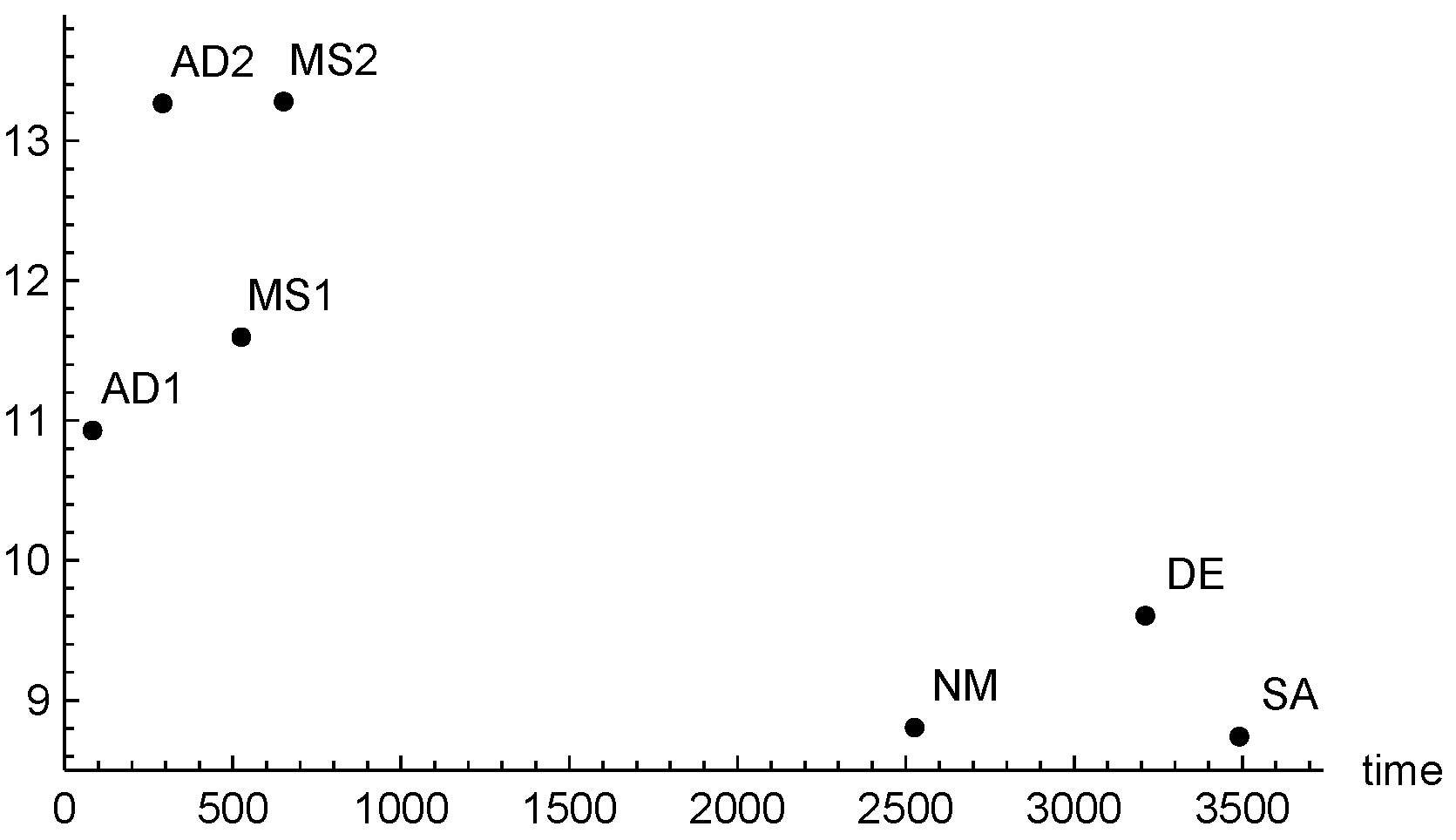
First, we analyze the effect of the chosen tolerance on Class 2 methods. The experiments confirm the expectation that stronger tolerance requests, which pay in terms of larger execution time, in general lead to more accurate results. The comparison of the performances of Class 1 and Class 2 methods shows that the accuracy of MS2 and AD2 does not appear to suffer too much with respect to the accuracy of Class 1 methods, in spite of the fact that they enjoy a much smaller execution time.

In order to summarize the results of the experimentation, we plot in Figure 3 the average of all the values of $lerr$, taken as a measure of the methods accuracy on all the problems, versus the averaged $time$. The larger the ordinate value, the more accurate the method.

Figure 3. Average $lerr$ (taken as a measure of accuracy) versus $time$.

From the figure we see that, on average, the adaptive procedure AD2 not only is faster, but also gives comparable accuracy with MS2. This is due to the fact that the computational effort of AD2 is focused where it is more useful and is not wasted.

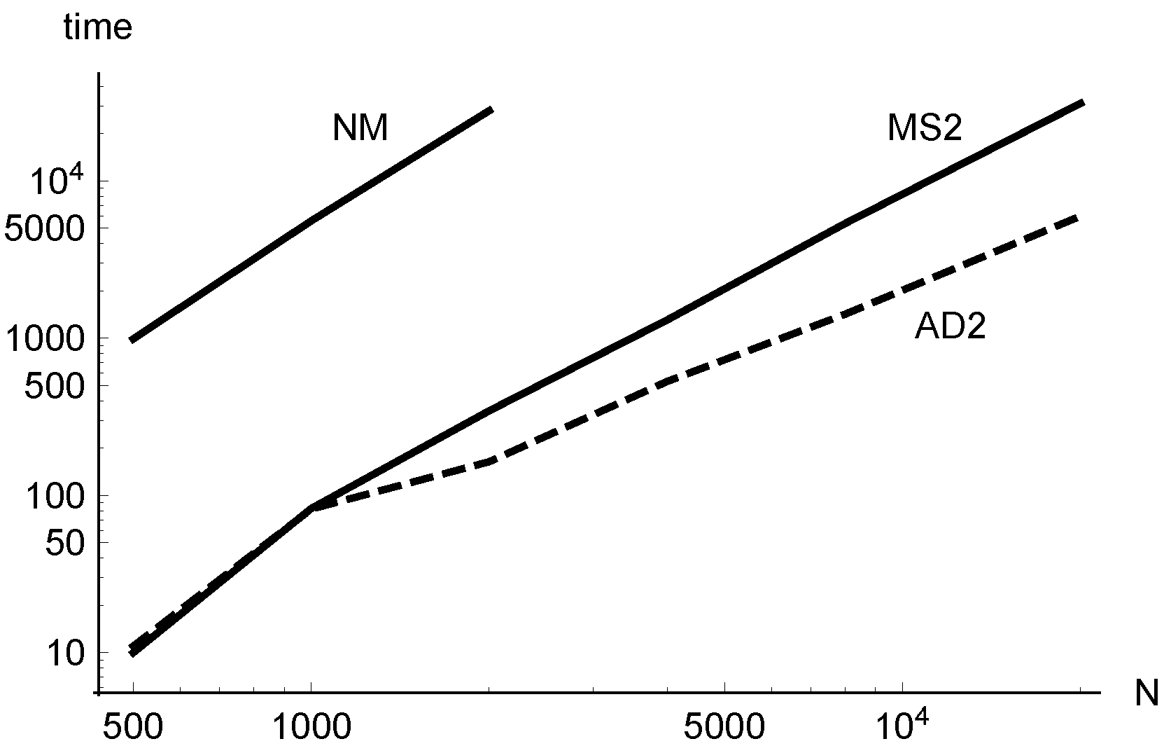
To study how $time$ depends on N, we need data corresponding to large values of N. A problem for which it is possible to obtain these data is the symmetric NMF applied to clustering. In fact, in this case it is easy to construct problems of the same type with increasing dimensions.

Figure 4 gives an idea of the time performance of the methods when they are applied to the cluster problem $C_2$. Class 2 methods have been run with increasing dimensions until $n=2000$, corresponding to size $N=$ 20,000. The execution times of AD2 (dashed line) and MS2 (solid line) are plotted together with the times of NM (solid line), chosen as the representative of Class 1 for $N\le 2000$ (larger dimensions for Class 1 methods could not be considered). For the lower dimensions, the use of the adaptive method does not give advantages, because of the initialization overhead (due to the $6\lambda$ iterations performed for stabilization before starting the adaptive strategy). This is shown by the overlap of the plots of AD2 and MS2 in the initial tract.

Figure 4. Log-log plot of the execution times of AD2, MS2, and NM versus N.

The lines which appear in the log-log plot suggest that the asymptotical behavior of the computational cost for increasing N is of the form $\alpha N^{\beta }$. Very similar values of $\beta$ suggest that the costs of MS2 and NM have roughly the same order, while the cost of AD2 has a lower order. It is evident that the multiplicative constant $\alpha$, whose log is readable from the vertical offset of the lines, of MS2 and AD2 is very lower than the one of NM.

6. Conclusions

In this paper an adaptive strategy, called AD, has been introduced for finding the global minimum of a polynomial function expressed through the Frobenius norm of matrices and tensors. The strategy is based on a heuristic approach to the Multistart algorithm. To compare the proposed method with some classical library methods, an extensive experimentation has been performed on both nonnegatively constrained and unconstrained problems, which include the nonnegative factorization of matrices and tensors and the determination of the tensor rank associated to the matrix product complexity. The proposed method allows a considerable saving of the computational time and comparable accuracy with respect to classical procedures.