Image Error Concealment Based on Deep Neural Network

Abstract

In this paper, we propose a novel spatial image error concealment (EC) method based on deep neural network. Considering that the natural images have local correlation and non-local self-similarity, we use the local information to predict the missing pixels and the non-local information to correct the predictions. The deep neural network we utilize can be divided into two parts: the prediction part and the auto-encoder (AE) part. The first part utilizes the local correlation among pixels to predict the missing ones. The second part extracts image features, which are used to collect similar samples from the whole image. In addition, a novel adaptive scan order based on the joint credibility of the support area and reconstruction is also proposed to alleviate the error propagation problem. The experimental results show that the proposed method can reconstruct corrupted images effectively and outperform the compared state-of-the-art methods in terms of objective and perceptual metrics.

1. Introduction

Reliably delivering high-quality multimedia data is a significant task for applications such as television broadcasting. However, the transmission channel is not always satisfactory. When multimedia data are transmitted over error-prone channels or bandwidth-limited channels, packet loss will greatly reduce the quality of the received multimedia data. A straightforward way to alleviate this problem is to retransmit that multimedia data. However, retransmission is unavailable in many practical applications, especially under certain real-time constraints such as live broadcast and multicast. Therefore, it is crucial to develop error concealment techniques to reconstruct the received error multimedia data in order to guarantee the quality of transmission.

Image error concealment (EC), as a post-processing method, reconstructs the missing pixels without the need to modify the encoder or change the channel conditions [1]. The basic idea behind EC is to predict the missing pixels by using the correctly received ones in the current frame or adjacent frames based on the spatial or temporal correlations. According to which kind of correlation is utilized, EC methods can be classified into three categories: spatial EC (SEC) [2,3,4,5,6,7,8,9,10,11,12,13,14,15], temporal EC (TEC) [16,17,18,19,20,21,22], or spatial–temporal EC (STEC) [23,24,25,26]. In the case that the neighbor frames are not available, the SEC methods only use the information extracted from the neighboring pixels of the missing ones in the current frame. Here, the TEC methods purely take advantage of the temporal correlation. The missing blocks are replaced with similar areas in the previously decoded frames. STEC methods can be considered as a combination of SEC and TEC, which exploits the correlation in both spatial and temporal domains. Considering that the temporal correlation or information does not always exist (for example, the corrupted images are still images), therefore, we focus on the SEC methods in this paper and reconstruct the missing pixels using only the spatial information.

SEC methods reconstruct the missing pixels by utilizing the correctly received ones in adjacent regions based on the natural images that have local correlation. Sun and Kwok [4] reconstructed the missing blocks by utilizing the spatially correlated edge information, which was extracted from a large local neighborhood of surrounding pixels. This method also can be viewed as an alternating projection onto convex sets (POCS) method. It performs well in reconstructing the major edges, but may incur objectionable false edges in smooth areas. Li and Orchard [6] proposed a sequential recovery method based on orientation adaptive interpolation (OAI). In this method, the previously recovered pixels can be used in the recovery afterward. This sequential pixel-wise manner can improve the capability of capturing important edge features from the surroundings. Jan et al. [7] concealed missing image blocks based on the concept of visual clearness (VC) of edge. They used Hough transform to find the relevant edges and employed the visually clearest ones for interpolating. As several directional interpolations are combined through visual clearness, more complex textures can be reconstructed. However, it is hard to accurately determine the visual clearness. Shirani et al. [27] treated natural images as Markov random fields (MRF). They reconstructed the missing pixels by exploiting the information from wide neighborhoods. This method gained a visually comfortable but sometimes may blur details. In [28], Koloda et al. suggested using multivariate kernel density estimation (MKDE) to conceal the corrupted images. Furthermore, a minimum mean square error (MMSE) estimator was exploited to recover missing pixels in [10]. The estimator employs a probability density function obtained by kernel density estimation (KDE). More recently, Liu et al. [8] reconstructed missing pixels through an adaptive linear predictor (ALP). The predictor can automatically tune its order and support shape according to the local contexts. In addition, they proposed an uncertainty-based scan order to alleviate the error propagation problem. However, they only considered the uncertainty of the neighbor pixels of the missing pixels, while the credibility of the reconstruction also influences the error propagation. In [29], over-completed dictionaries were learned for recovering missing pixels. They trained two dictionaries individually for the missing part and the available part, and they reconstructed the missing part through a local correlation model that was trained to bridge the two dictionaries. In [14], they proposed a Gaussian-weighted non-local texture similarity measure to obtain multiple candidate patches for each target patch, using the non-local texture measure. Therefore, their algorithm is capable of reproducing the underlying textural details.

Neural network, as a powerful model, has been proved to be effective in EC tasks [15,20,21]. Shao and Chen [20] exploited a general regression neural network (GRNN) to estimate the motion vectors of the corrupted macro-blocks (MBs). They collected the adjacent motion vectors of the corrupted MBs for training the GRNN at first. Then, the corrupted MBs were reconstructed through the corresponding motion vectors, which were estimated by the GRNN. In [21], deep neural networks were used to predict the optical flow for video error concealment. They designed two parallel networks to separately process the horizontal and vertical motion fields of the optical flows of the previous frame. Then, the combined output of the two networks was used to reconstruct the corrupted portion of the video frames. Both of the aforementioned two methods reconstructed corrupted images by utilizing the information from the adjacent frames of the video. However, reliable adjacent frame information is not available in some situations. For example, corrupted images are not from videos.

Unlike [20,21], we reconstructed the missing pixels through only utilizing the information from the current frame in this paper. We propose a novel EC technique to reconstruct the missing pixels via training a deep neural network. Considering that the natural images have local correlation and non-local self-similarity, we used the local information to predict the missing pixels and the non-local information to correct the predictions. The designed neural network can be divided into two parts: the prediction part and the auto-encoder (AE) part. The first part utilizes the local correlation among pixels to predict the missing ones. The other part extracts image features, which are used to collect similar samples from the whole image. In addition, we propose a novel adaptive scan order based on the joint credibility of the support area and reconstruction to alleviate the error propagation problem. The experimental results show that the proposed algorithm can reconstruct corrupted images effectively and outperforms the compared state-of-the-art methods in terms of peak signal-to-noise ratio (PSNR) and structural similarity (SSIM).

2. Problem Formulation

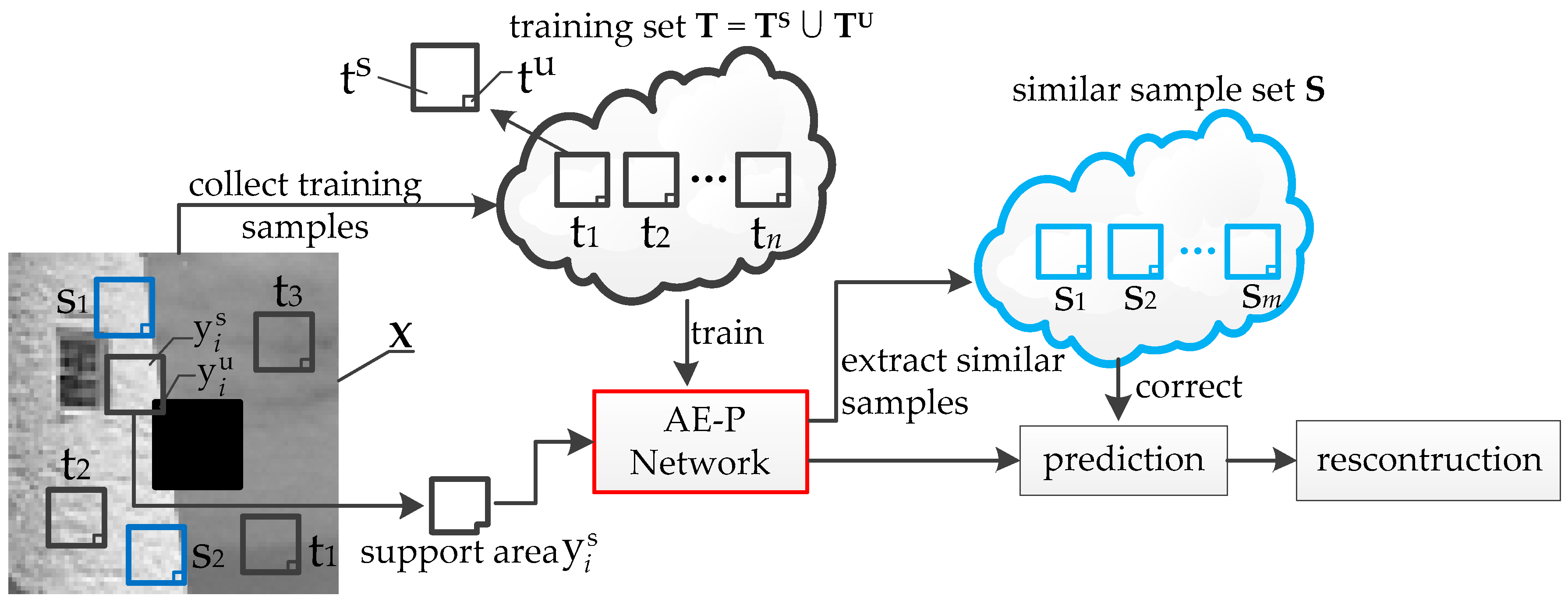
Similar to the other SEC methods, we reconstructed the missing pixels using the correctly received ones. More specifically, we used the local information to predict the missing pixels and non-local information to correct the predictions in this paper.

Let $\mathbf{O}$ be the original image, $\mathbf{X}$ be the corresponding corrupted image, and $\mathbf{X}$ can be divided into an available part, $\mathbf{S}$, and an unavailable part, $\mathbf{U}$; that is, $\mathbf{X}=\mathbf{U}$ ∪ $\mathbf{S}$. Therefore, the EC problem can be considered to reconstruct the unavailable part $\mathbf{U}$ through utilizing the information from the available part $\mathbf{S}$. Without a loss of generality, we suppose that only one pixel is reconstructed at a time. Define ${\mathbf{y}}_i$ as a pixel group that contains pixel $i$, which is located on the contour of $\mathbf{U}$, as shown in Figure 1. Note that ${\mathbf{y}}_i$ can be regarded as a combination of ${\mathbf{y}}_i^{\mathrm{s}}$ and ${\mathbf{y}}_i^{\mathrm{u}}$. ${\mathbf{y}}_i^{\mathrm{u}}$ is the pixel set that contains the missing pixels, and here, it is actually the missing pixel i, since we reconstruct only one pixel at a time. ${\mathbf{y}}_i^{\mathrm{s}}$ is a pixel set formed by the adjacent and available neighbors of ${\mathbf{y}}_i^{\mathrm{u}}$. We call ${\mathbf{y}}_i^{\mathrm{s}}$ a support area of ${\mathbf{y}}_i^{\mathrm{u}}$, since ${\mathbf{y}}_i^{\mathrm{s}}$ can be regarded as the spatial context of ${\mathbf{y}}_i^{\mathrm{u}}$. Obviously, we can estimate ${\mathbf{y}}_i^{\mathrm{u}}$ from ${\mathbf{y}}_i^{\mathrm{s}}$ by utilizing the local correlation of natural images. Considering that natural images have non-local self-similarity properties, in our method, the non-local information is also used in the image reconstruction. We use the non-local information to correct the predictions. The reconstruction of missing pixel ${\mathbf{y}}_i^{\mathrm{u}}$ can be defined as:

$${\widehat{\mathbf{y}}}_i^{\mathrm{u}}=\mathit{\varphi }({\mathbf{y}}_i^{\mathrm{s}})+\lambda \mathit{F}({\mathbf{S}}_i)$$

(1)

where ${\mathbf{y}}_i^{\mathrm{s}}$ is the support area of ${\mathbf{y}}_i^{\mathrm{u}}$ and ${\mathbf{S}}_i$ is a set of samples, which are similar to ${\mathbf{y}}_i^{\mathrm{s}}$. Model $\mathit{\varphi }(·)$ is used to predict the missing pixels through the corresponding support areas. Function $\mathit{F}(·)$ uses the similar sample set ${\mathbf{S}}_i$ to correct the predictions of $\mathit{\varphi }(·)$. $\lambda$ is a factor that balances the corrections and predictions, ${\widehat{\mathbf{y}}}_i^{\mathrm{u}}$ is the final reconstruction that will be used to replace the missing pixel.

In addition, under the sequential framework, the corrupted images are reconstructed pixel by pixel in sequence. The sequence, which is often called a scan order, is very important to the reconstruction performance, since it determines the available context of each missing pixel. After each pixel is reconstructed, we update the available part $\mathbf{S}$ and the unavailable part $\mathbf{U}$. The EC task is accomplished when the unavailable part $\mathbf{U}$ becomes an empty pixel set.

Therefore, the focus of our work is to build a model $\mathit{\varphi }(·)$ for predicting the missing pixels, find an approach to search for useful non-local information, and use it to correct the predictions. Moreover, it is also an important issue to determine an appropriate scan order in our work.

3. Our Proposal

In this work, we propose an EC method that take into account both the local and non-local information in the reconstruction of the corrupted images. More specifically, we exploit the local information to predict the missing pixels and the non-local information to correct the predictions. In our method, a deep neural network is designed to serve as the prediction model $\mathit{\varphi }(·)$ to achieve the EC purpose. The designed neural network can be divided into two parts: the prediction part and the auto-encoder (AE) part. The prediction part utilizes the local correlation among pixels to predict the missing ones. The AE part is used to extract the image features. Through those extracted features, we collected similar samples from the whole image. Since the designed neural network can extract image features through the AE part and predict missing pixels using the prediction part, we call it an AE-P network.

As illustrated in Figure 2, given a corrupted image $\mathbf{X}$, we first collect all the possible samples from the available area to serve as the training set $\mathbf{T}=[{\mathrm{t}}_1,{\mathrm{t}}_2,\dots ,{\mathrm{t}}_n]$, and each sample $\mathrm{t}$ in set $\mathbf{T}$ can be regarded as a combination of an available part ${\mathrm{t}}^{\mathrm{s}}$ and a missing part ${\mathrm{t}}^{\mathrm{u}}$. Here, it should be pointed out that the true value of ${\mathrm{t}}^{\mathrm{u}}$ in training set $\mathbf{T}$ is known. Therefore, the training set $\mathbf{T}$ can be divided into two subsets ${\mathbf{T}}^{\mathrm{s}}$ and ${\mathbf{T}}^{\mathrm{u}}$, which are composed of ${\mathrm{t}}^{\mathrm{s}}$ and ${\mathrm{t}}^{\mathrm{u}}$, respectively. Then, the collected training set $\mathbf{T}$ is used to train the designed AE-P network. More specifically, we train the AE part network through unsupervised learning and the prediction part network through supervised learning. Let ${\mathbf{y}}_i^{\mathrm{u}}$ be the current missing pixel on the contour of the unavailable region, and ${\mathbf{y}}_i^{\mathrm{s}}$ be the corresponding support area. When we input ${\mathbf{y}}_i^{\mathrm{s}}$ into the trained AE-P network, on the one hand, we can get the prediction $\mathit{\varphi }({\mathbf{y}}_i^{\mathrm{s}})$ of the missing pixel through the prediction part network. On the other hand, the AE part network extracts the features of ${\mathbf{y}}_i^{\mathrm{s}}$ by comparing the similarities in the feature domain and the pixel domain. Thus, we searched for samples similar to ${\mathbf{y}}_i^{\mathrm{s}}$ from the whole image, which served as a similar sample set, $\mathbf{S}$, as illustrated in the blue box in Figure 2. Then, we used these similar samples to correct the prediction $\mathit{\varphi }({\mathbf{y}}_i^{\mathrm{s}})$ based on the non-local similarity of the natural images. Therefore, the final reconstruction ${\widehat{\mathbf{y}}}_i^{\mathrm{u}}$ is determined through combining the prediction and correction, as shown in Formula (1). In this way, both the local and non-local information are taken into account for reconstruction. In addition, to alleviate the error propagation problem, we proposed an adaptive scan order based on the joint credibility of the support area and the reconstruction.

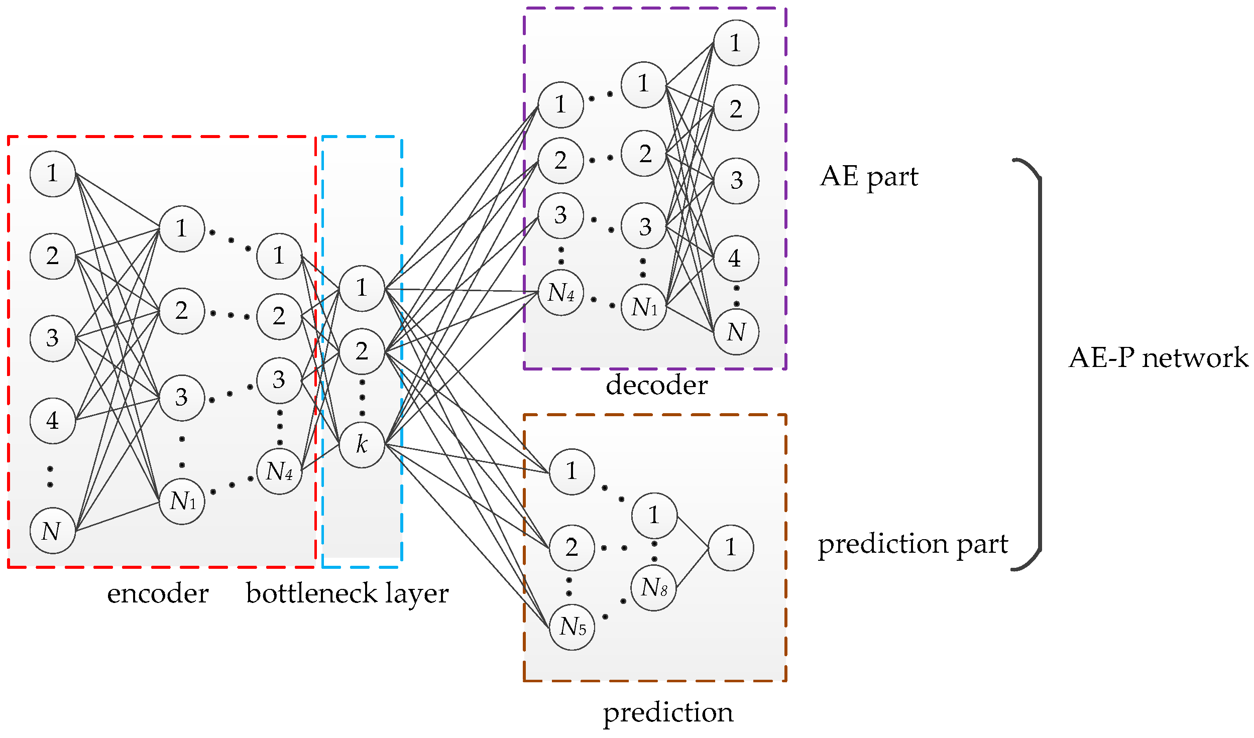
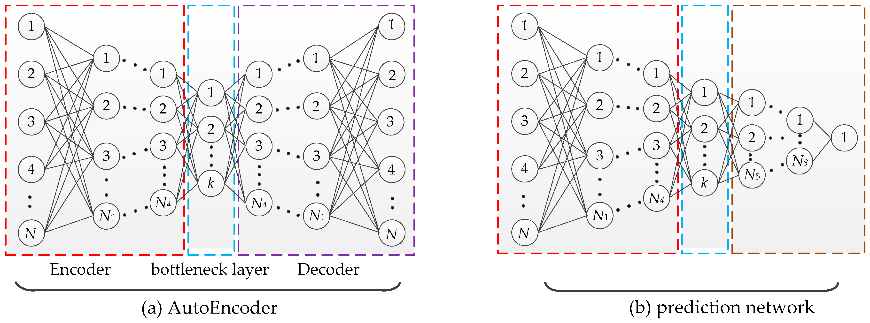
3.1. Design of AE-P Neural Network

In this paper, a deep neural network named the AE-P network is designed to achieve the EC purpose. The network can accomplish two tasks. One is to predict the missing pixels through using the local correlation between the missing pixels and the available pixels. The other is to extract the image features so as to search for feature similar samples. The second task is accomplished through AE, which is short for auto-encoder, as proposed by Hinton [30] in 2006. The AE is an unsupervised learning method that reconstructs the input signal at the output side so as to realize the dimensionality reduction of complex data. A typical AE network consists of an encoder and a decoder. Between the encoder and decoder is the bottleneck layer, which we focus on in our method, since it is the most compact feature representation of input data. The encoder is from the input layer to the bottleneck layer, and the decoder is from the bottleneck layer to the output layer. This bottleneck layer is exactly the data representation after dimensionality reduction. Compared with the traditional dimension reduction methods such as principal component analysis (PCA), the AE network can extract high-level features of the data due to the excellent non-linear representation power of the deep neural network.

To train the AE-P network, we firstly use the subset ${\mathbf{T}}^{\mathrm{s}}$ to train the AE part network through unsupervised learning. Suppose that the samples in ${\mathbf{T}}^{\mathrm{s}}$ are $N$-dimensional data; then, the dimension of the input layer and the output layer of the AE network are $N$, correspondingly. Then, we need to determine the dimension of the bottleneck layer, which is a significant issue in the design of the AE network. In general, the lower dimension of the bottleneck layer, the higher the efficiency of coding at the expense of more information loss. So, it is necessary to balance the coding efficiency and information loss. In our method, we set the dimension of the bottleneck layer to be half that of the input layer. The structure of the deep AE network in our method is shown in Figure 3a, and the optimization of AE network is defined as:

$$\arg \min {\Vert {\mathrm{t}}^{\mathrm{s}}-{\widehat{\mathrm{t}}}^{\mathrm{s}}\Vert }^2$$

(2)

where ${\mathrm{t}}^{\mathrm{s}}$ is the one of sample of subset ${\mathbf{T}}^{\mathrm{s}}$. ${\widehat{\mathrm{t}}}^{\mathrm{s}}$ is the corresponding output of the AE network. As can be seen from the formula, the objective of the optimization of the AE network is to minimize the mean square error between the input and the output.

Next, we use the subset ${\mathbf{T}}^{\mathrm{u}}$ as the corresponding label set of ${\mathbf{T}}^{\mathrm{s}}$ to train the prediction part network through supervised learning. Figure 3b is the structure of the prediction network. The input of the prediction network ${\mathrm{t}}^{\mathrm{s}}$ is the available part of the training samples, which are the same as the input of the AE network. The output are the predictions of the unavailable part pixels of the corresponding samples. Since we reconstruct only one missing pixel at a time, the output layer dimension of the prediction network is one, representing the prediction of the missing pixel. The optimization of AE network is defined as:

$$\arg \min {\Vert {\mathrm{t}}^{\mathrm{u}}-{\widehat{\mathrm{t}}}^{\mathrm{u}}\Vert }^2$$

(3)

where ${\mathrm{t}}^{\mathrm{u}}$ represents the true values of the missing pixels, and ${\widehat{\mathrm{t}}}^{\mathrm{u}}$ represents the corresponding predictions of the prediction network.

Consider that the inputs of the two aforementioned networks are exactly the same; therefore, the front parts of the two networks are designed to be the same. Thus, a new network, which we call the AE-P network, is formed through combining the two networks and sharing the same part. The structure of the AE-P network is shown in Figure 4. The trained AE-P network can predict the missing pixels and extract image features at the same time. As can be observed from the structure, the front part of the AE-P network is the AE, and the network has two different output branches. We first trained the AE network through unsupervised learning. This network corresponds to the first branch of the AE-P network. Then, we kept the parameters of the encoder and only updated the parameters of the prediction part to train the prediction network through supervised learning, which corresponds to the second branch of the AE-P network.

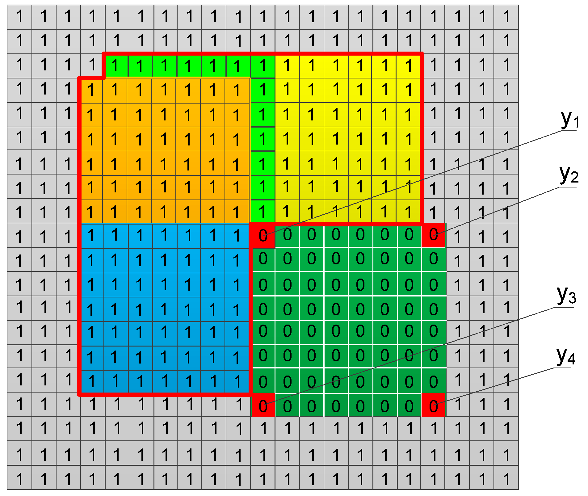
3.2. Training Data Collection

For training the designed AE-P network, we need a large number of samples. In order to collect appropriate training data, a template matching scheme is utilized to match and collect samples from the whole image. A challenging problem of the scheme is how to design the template shape to get the maximum available information. Similar to many SEC methods, templates with a square shape, as shown in Figure 5a, are widely used in training data collecting. The corresponding context of the missing pixel is shown in the blue dotted box in Figure 5b. It can be observed that only the available pixels in area A, which is part of the context, are used to reconstruct the current missing pixel. However, it is true that the pixels in areas B and C also have high correlation with the missing pixel. Thus, the available pixels in areas B and C should also be taken into account in image reconstruction. Since more available information is considered, the reconstruction of the missing pixel will be more reliable.

In order to get more available information from the context, eight templates with different shapes are designed in our method, as shown in Figure 6. These eight templates can be embedded around the missing pixels to augment the information collected from the context. Unlike square templates, which can only match one support area from the context for each missing pixel, we can collect multiple support areas. As illustrated in Figure 7, four support areas, ${\mathbf{y}}_i^{{\mathrm{s}}_1}$, ${\mathbf{y}}_i^{{\mathrm{s}}_2}$, ${\mathbf{y}}_i^{{\mathrm{s}}_3}$, and ${\mathbf{y}}_i^{{\mathrm{s}}_4}$ around the current missing pixel ${\mathbf{y}}_i^{\mathrm{u}}$ can be collected through matching the eight templates in the context. The available information obtained by these four support areas is shown in the blue box in Figure 7. For each support area, a reconstruction will be generated through the trained AE-P network. By combining the reconstructions of these support areas, the final reconstruction is therefore determined through all the available pixels of these support areas. The final reconstruction of the missing pixel ${\mathbf{y}}_i^{\mathrm{u}}$ is determined as:

$${\widehat{\mathbf{y}}}_i^{\mathrm{u}}=\frac{1}{N}{\displaystyle \sum _{j=1}^N{\widehat{\mathbf{y}}}_i^{{\mathrm{u}}_j}}$$

(4)

where ${\widehat{\mathbf{y}}}_i^{{\mathrm{u}}_j}$ is the reconstruction corresponding to the support area ${\widehat{\mathbf{y}}}_i^{{\mathrm{s}}_j}$, $N$ is the number of matched support areas, and ${\widehat{\mathbf{y}}}_i^{\mathrm{u}}$ is the final reconstruction of the missing pixel. This formula shows that the final reconstruction of the missing pixel is the average of the reconstructions corresponding to all of the collected support areas.

Eight templates with different shapes are utilized to collect training data for training the AE-P network in the proposed method. However, the relative location of the missing pixels and the corresponding support area are different among the collected samples. In order to train the AE-P network, we normalized all the collected training samples into a standard shape through rotating and flipping. As shown in Figure 6, we defined the template shape down-left as the standard shape and transformed all the collected training samples into the standard shape. For example, the procedure of transforming the shape from up-left into the standard shape is shown in Figure 8.

In our method, we collected the training data from the available regions of the input-corrupted images. Specifically, we firstly used the designed eight templates to match all the possible samples in the available region. Next, we normalized the collected samples into the standard shape through the aforementioned processing. Then, the normalized collected samples could serve as the training data for training the AE-P network.

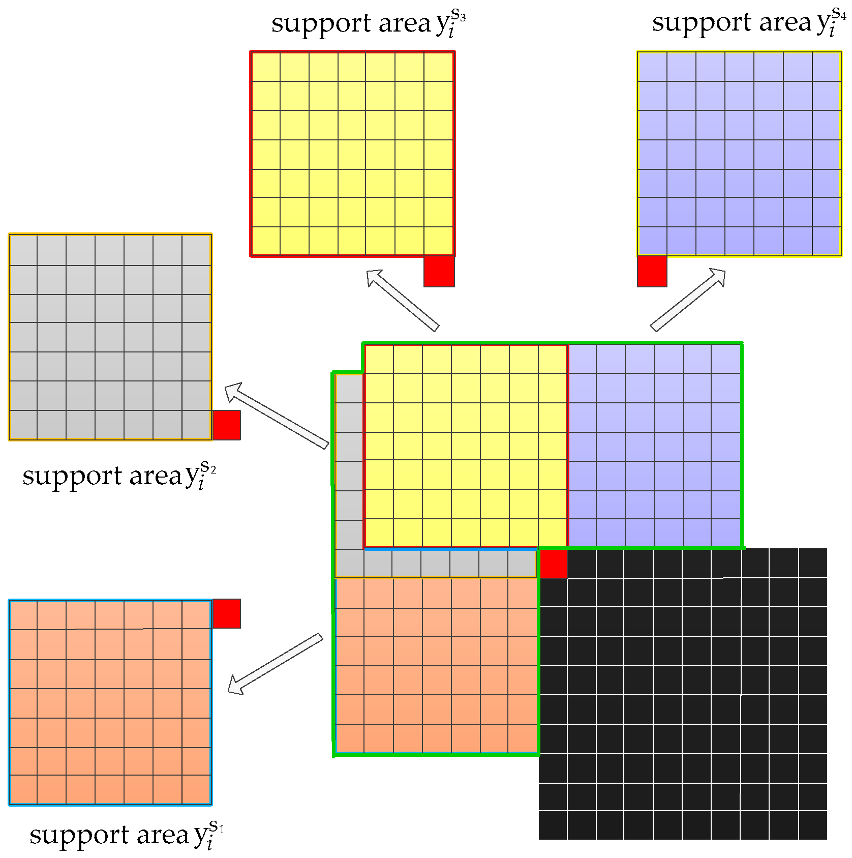
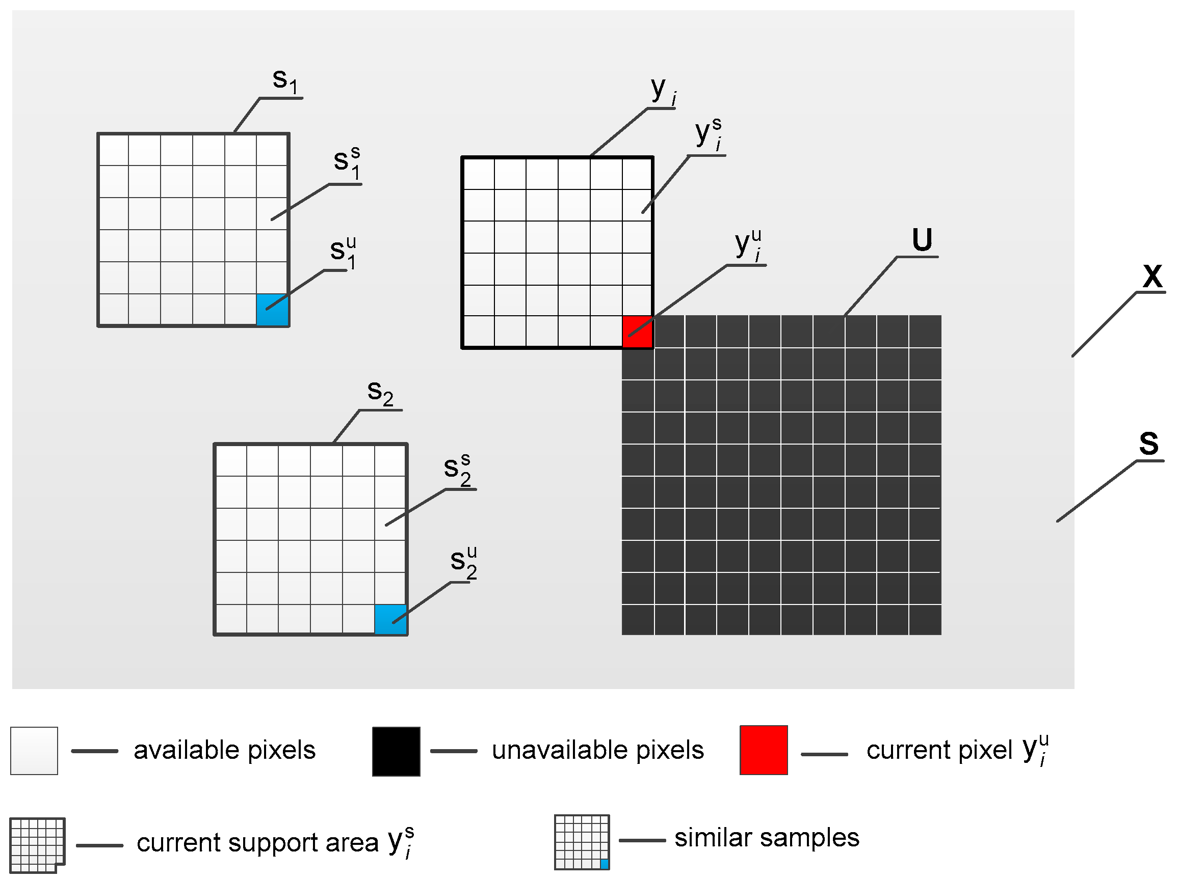
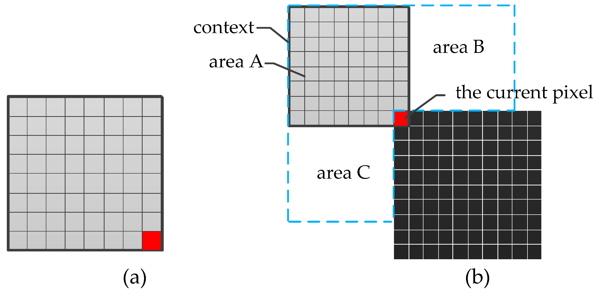
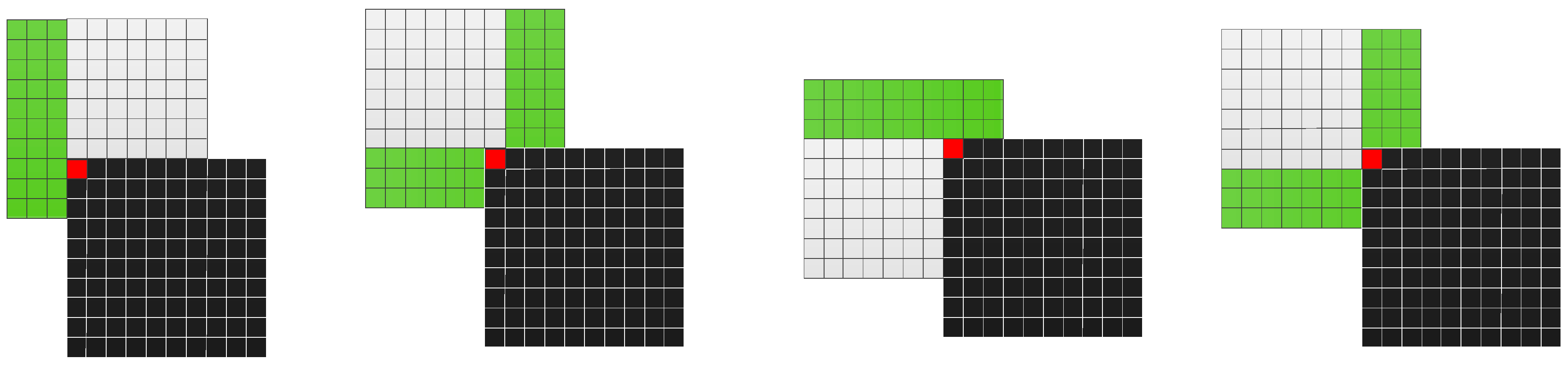
3.3. Similar Data Collection

Error concealment is an ill-posed inverse problem, as the true values of missing pixels are unavailable in practice. Thus, the prediction error, which will reduce the reconstruction performance, is inevitable. In the proposed method, we utilized the AE-P network to reconstruct the missing pixels. Considering that the AE-P network has similar outputs for similar inputs, we assumed that the prediction errors for similar inputs were similar. Based on this assumption, we searched for the data similar to the current input of the AE-P network. Then, the network prediction errors of those data could be used to correct the prediction of the current input. This can reduce the prediction error and improve the reconstruction performance. Many methods such as those in [8,28] collected similar samples in pixel space. However, it is not reliable to measure the similarity of samples in pixel space, since the pixel value in the pixel space represents the gray value. In pixel space, the collected similar samples may only be similar in pixel value, but not in the feature, especially in the texture region. To avoid the drawbacks of collecting similar samples in pixel space, we defined the feature space and collected similar samples in this space. The feature space is composed of the sample features, which are determined through the bottleneck layer of the trained AE-P network. In feature space, the feature similarity between samples is easy to measure, so we can collect samples with more similar features. In addition, the computational complexity is greatly reduced, since the dimension of feature space is much lower than that of pixel space.

The Euclidean distance is used to measure the similarity between samples and the current support area in feature space. We defined $\mathbf{p}$ as the current support area of the current missing pixel, and $\mathbf{q}$ as a collected sample with the same shape as $\mathbf{p}$. $f_{\mathbf{p}}$ and $f_{\mathbf{q}}$ are corresponding feature representations determined through the bottleneck layer of the trained AE-P network; then, the Euclidean distance $D_f(\mathbf{p},\mathbf{q})$ is used to measure the similarity of $\mathbf{p}$ and $\mathbf{q}$ as:

$$D_f(\mathbf{p},\mathbf{q})=\sqrt{{\displaystyle \sum _{i=1}^k{(f_{\mathbf{p}}^i-f_{\mathbf{q}}^i)}^2}}$$

(5)

where $f_{\mathbf{p}}^i$ and $f_{\mathbf{q}}^i$ are the i^th values of $f_{\mathbf{p}}$ and $f_{\mathbf{q}}$, respectively. $k$ is the dimension of the feature space. The formula shows that the smaller the distance, the more similar $\mathbf{p}$ and $\mathbf{q}$ are in the feature space. Formula (5) may fail at measuring the sample similarity in pixel space, since some samples are similar in feature space but very different in pixel space. Therefore, we required these collected similar samples as determined by Formula (5) to be similar to $\mathbf{p}$ in pixel space. We also used the Euclidean distance to measure the similarity between the collected samples and the current support area in pixel space. In order to make the measurement of the similarity in pixel space more reliable, some adjacent pixels of the missing pixel were added in the similarity calculation. As illustrated in Figure 9, the green pixels are the added ones. The similarity between $\mathbf{p}$ and $\mathbf{q}$ in pixel space is defined as follows:

$$D_{\mathbf{p}}(\mathbf{p},\mathbf{q})=\sqrt{{\displaystyle \sum _{i=1}^n{({\overline{\mathbf{p}}}^i-{\overline{\mathbf{q}}}^i)}^2}}$$

(6)

where $\overline{\mathbf{p}}$ and $\overline{\mathbf{q}}$ are the augmented pixel sets corresponding to $\mathbf{p}$ and $\mathbf{q}$, respectively. $n$ is the pixel number of $\overline{\mathbf{p}}$. The formula shows that the smaller the distance, the more similar $\mathbf{p}$ and $\mathbf{q}$ are in pixel space.

Therefore, in our method, we first used Formula (5) to measure the similarity of samples to the current support area $\mathbf{p}$ in feature space and then collected the first n of the most similar samples to form the set ${\mathbf{S}}_j^{\mathrm{n}}=[{\mathbf{s}}_1,{\mathbf{s}}_2,{\mathbf{s}}_3,\dots ,{\mathbf{s}}_n]$. As shown below:

$${\mathbf{S}}_j^{\mathrm{n}}=\{{\mathbf{s}}_i|D_f(\mathbf{p},{\mathbf{s}}_i)<{\tau }_1\}$$

(7)

where ${\mathbf{s}}_i$ is the sample collected through matching the support area $\mathbf{p}$, and ${\tau }_1$ is the threshold selected in practice such that the first n = 500 closest samples were collected. Then, we used Formula (6) to calculate the similarity between the collected samples and the current support area $\mathbf{p}$ in pixel space; we only selected the first m most similar samples to serve as the similar sample set ${\mathbf{S}}_j=[{\mathbf{s}}_1,{\mathbf{s}}_2,{\mathbf{s}}_3,\dots ,{\mathbf{s}}_m]$, as shown below:

$${\mathbf{S}}_j=\{{\mathbf{s}}_i|D_{\mathbf{p}}(\mathbf{p},{\mathbf{s}}_i)<{\tau }_2,\hspace{1em}{\mathbf{s}}_i\in {\mathbf{S}}_j^{\mathrm{n}}\}$$

(8)

where ${\mathbf{s}}_i$ is the sample from set ${\mathbf{S}}_j^{\mathrm{n}}$, and ${\tau }_2$ is the threshold selected in practice such that the first m = 50 closest samples are selected from the set ${\mathbf{S}}_j^{\mathrm{n}}$. In this way, the similar samples we collected are similar both in feature space and pixel space.

3.4. Prediction Error Correct

Since samples that are similar to the current support area can be collected as mentioned in the last section, those similar samples are used to correct the prediction of the current support area. Let ${\mathbf{y}}_i^{\mathrm{u}}$ be the current missing pixel, and suppose that n support areas ${\mathbf{y}}_i^{{\mathrm{s}}_1}$, ${\mathbf{y}}_i^{{\mathrm{s}}_2}$, …, ${\mathbf{y}}_i^{{\mathrm{s}}_n}$ can be collected through matching the templates from the context. For each support area, we collected similar samples to correct the corresponding prediction. We defined ${\mathbf{S}}_j=[{\mathbf{s}}_1,{\mathbf{s}}_2,{\mathbf{s}}_3,\dots ,{\mathbf{s}}_m]$ as the similar sample set corresponding to the support area ${\mathbf{y}}_i^{{\mathrm{s}}_j}$. Suppose that ${\mathbf{s}}_{j,k}$ is the $k^{\mathrm{th}}$ samples in set ${\mathbf{S}}_j$; then, the prediction error $e_k$ of sample ${\mathbf{s}}_{j,k}$ is defined as:

$$e_k=\mathit{\varphi }({\mathbf{s}}_{j,k}^{\mathrm{s}})-{\mathbf{s}}_{j,k}^{\mathrm{u}}\hspace{1em}s.t.\hspace{1em}1\le k\le m$$

(9)

where ${\mathbf{s}}_{j,k}^{\mathrm{s}}$ is the available part of ${\mathbf{s}}_{j,k}$ and ${\mathbf{s}}_{j,k}^{\mathrm{u}}$ is the missing part of ${\mathbf{s}}_{j,k}$. $\mathit{\varphi }({\mathbf{s}}_{j,k}^{\mathrm{s}})$ is the prediction of ${\mathbf{s}}_{j,k}^{\mathrm{u}}$ through the trained AE-P network and ${\mathbf{s}}_{j,k}^{\mathrm{u}}$ is the true value, and $e_k$ is the prediction error produced by the network on the input ${\mathbf{s}}_{j,k}^{\mathrm{s}}$. Let set ${\mathrm{E}}_j=[e_1,e_2,e_3,\dots ,e_m]$ represent the error set corresponding to the input data set ${\mathbf{S}}_j$; then, the correction of the prediction $\mathit{\varphi }({\mathbf{y}}_i^{{\mathrm{s}}_j})$ is derived from the following formula:

$$a_j=-{\displaystyle \sum _{k=1}^m{c}_k}·e_k$$

(10)

where $c_k$ is the proportion of the prediction error $e_k$ in the whole correction $a_j$, and $c_k$ is determined by the similarity between sample ${\mathbf{s}}_k^{\mathrm{s}}$ and ${\mathbf{y}}_i^{{\mathrm{s}}_j}$. $c_k$ obeys the following formulas (11) and (12):

$${\displaystyle \sum _{k=1}^m{c}_k=1}$$

(11)

$$\frac{c_{n1}}{c_{n2}}=\frac{D_f({\mathbf{s}}_{j,n2}^{\mathrm{s}},{\mathbf{y}}_i^{{\mathrm{s}}_j})}{D_f({\mathbf{s}}_{j,n1}^{\mathrm{s}},{\mathbf{y}}_i^{{\mathrm{s}}_j})}$$

(12)

where $c_{n1}$ and $c_{n2}$ are the proportions corresponding to $e_{n1}$ and $e_{n2}$, ${\mathbf{y}}_i^{{\mathrm{s}}_j}$ is the current support area, and $D_f$ is used to calculate the Euclidean distance in feature space. Then, the reconstruction ${\widehat{\mathbf{y}}}_i^{{\mathrm{u}}_j}$ determined through the support area ${\mathbf{y}}_i^{{\mathrm{s}}_j}$ is shown as follows:

$${\widehat{\mathbf{y}}}_i^{{\mathrm{u}}_j}=\mathit{\varphi }({\mathbf{y}}_i^{{\mathrm{s}}_j})+a_j$$

(13)

For each support area, there will be a corresponding reconstruction generated by Formula (13). The final reconstruction ${\widehat{\mathbf{y}}}_i^{\mathrm{u}}$ of the missing pixel ${\mathbf{y}}_i^{\mathrm{u}}$ is the average of those reconstructions, as shown in Formula (4).

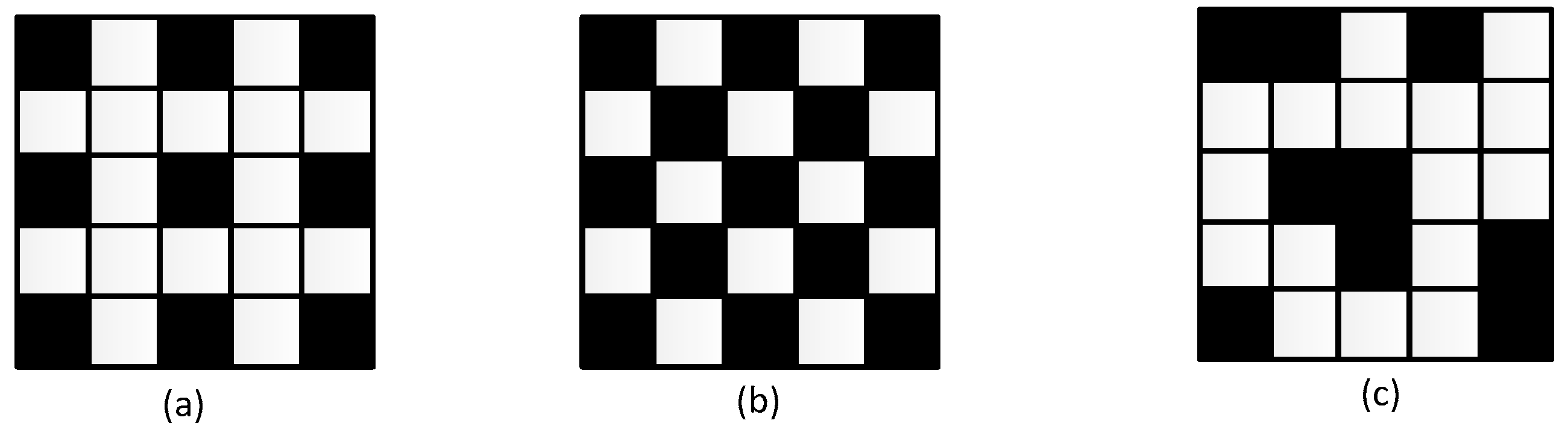
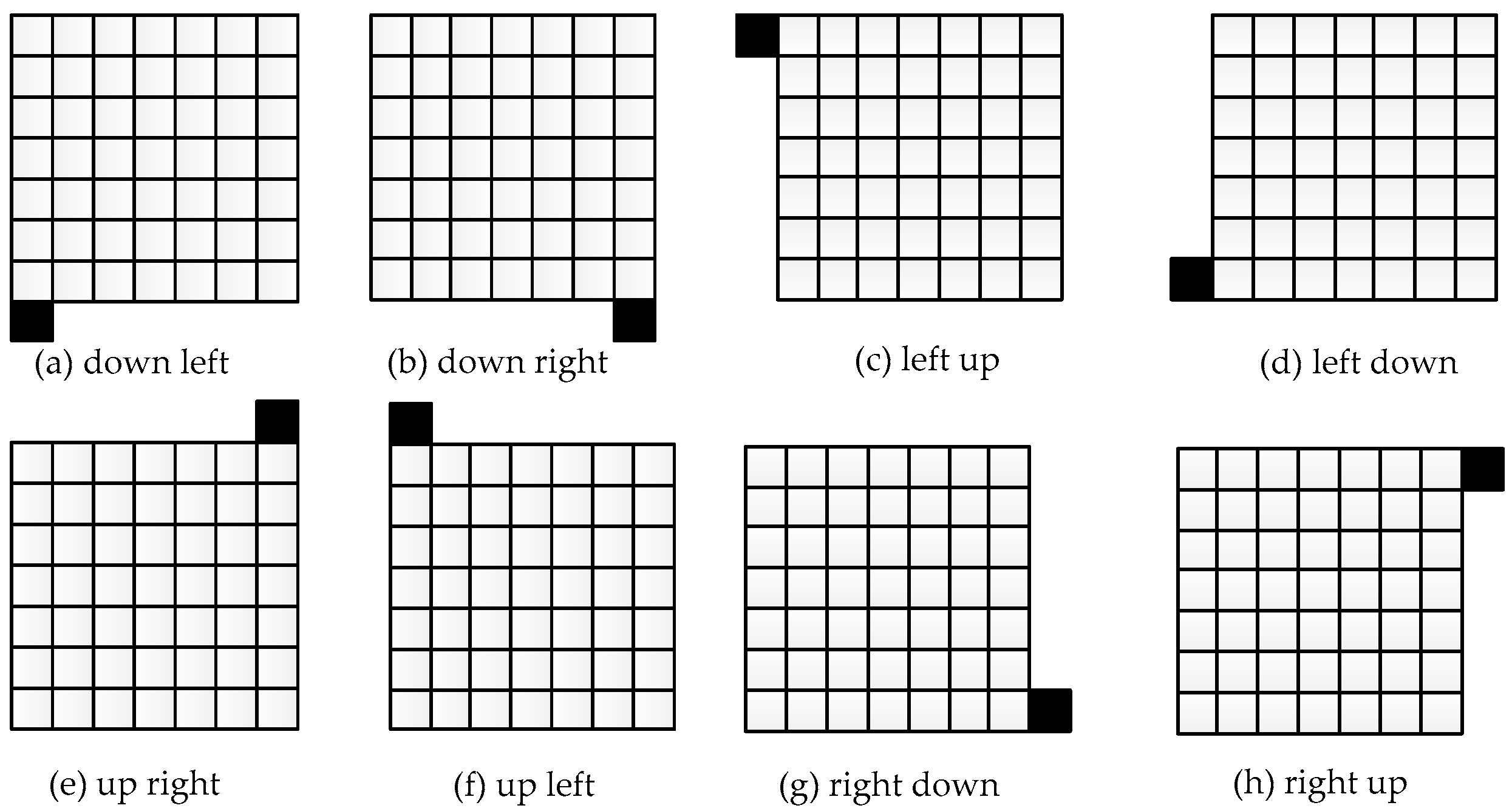
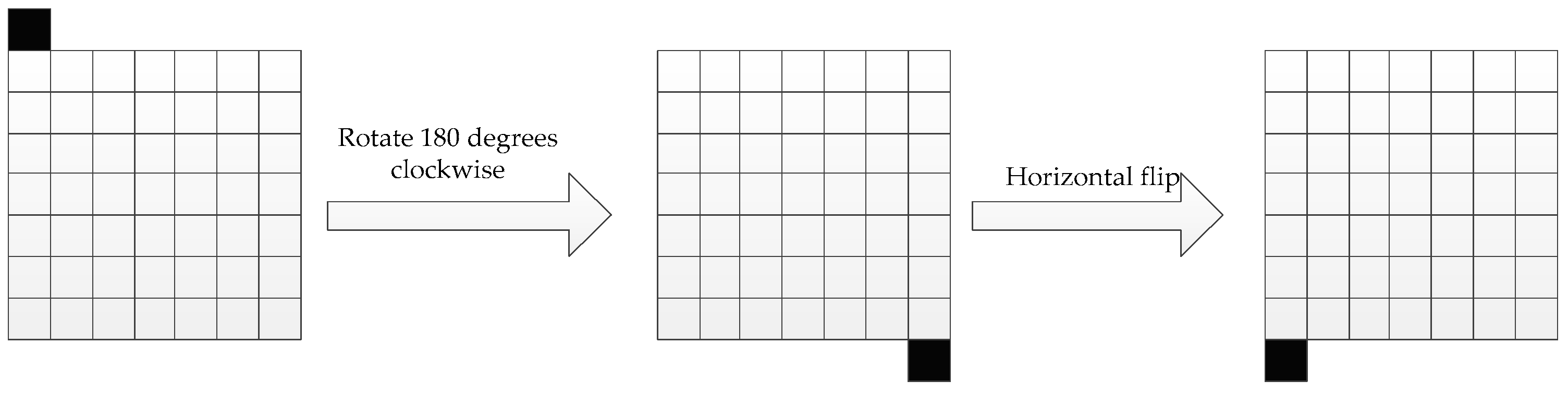
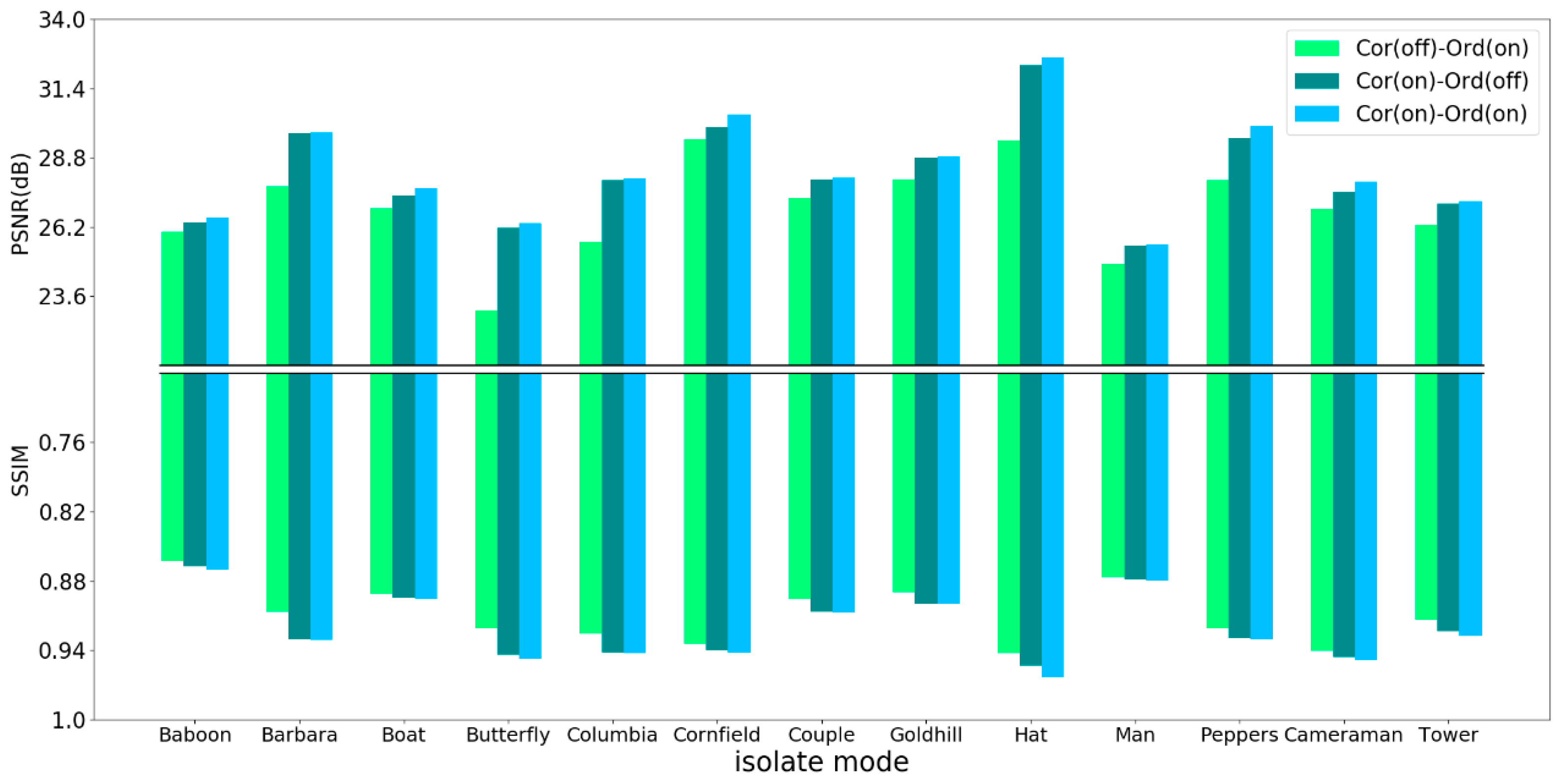
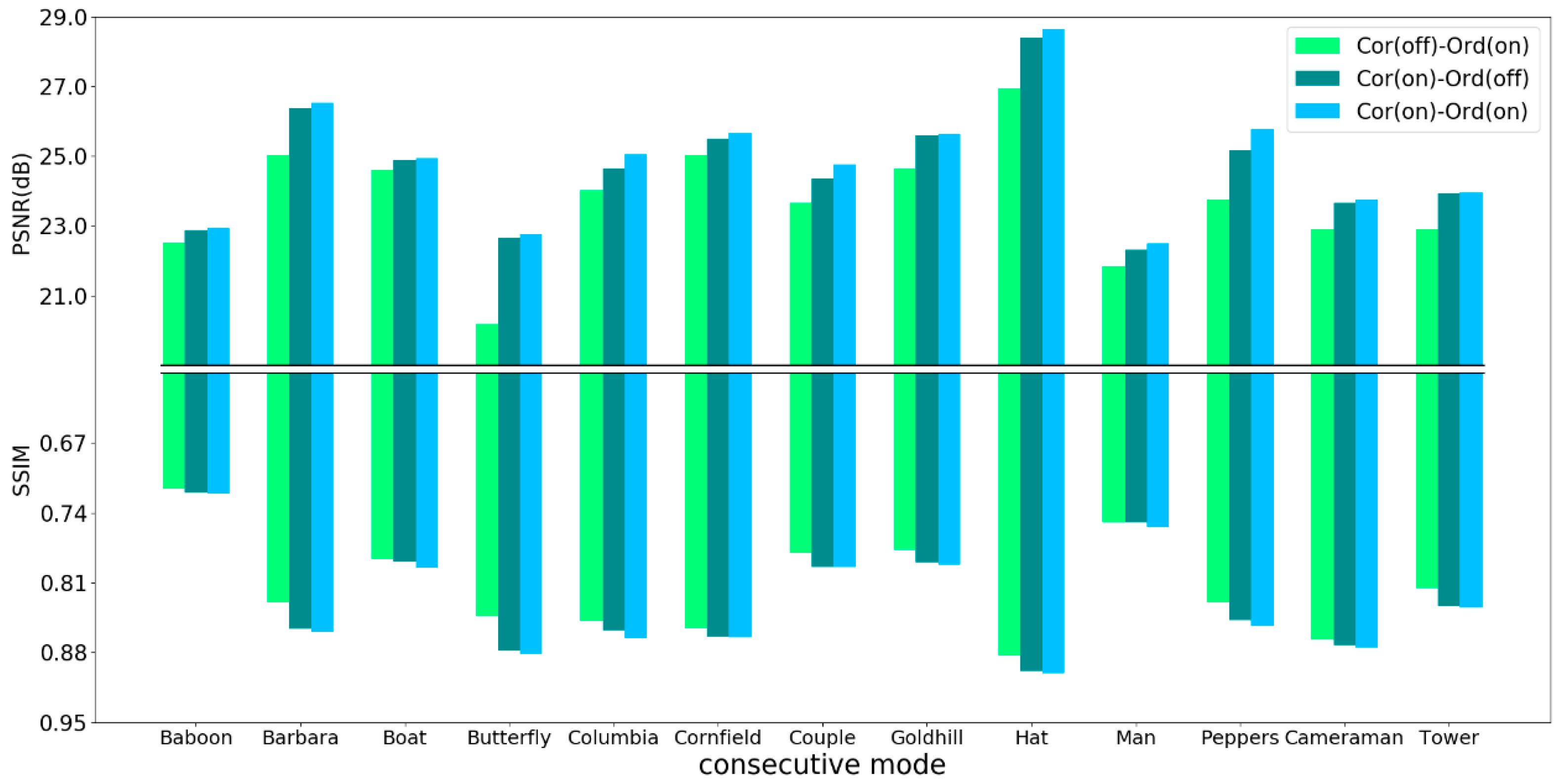
3.5. Adaptive Scan Order

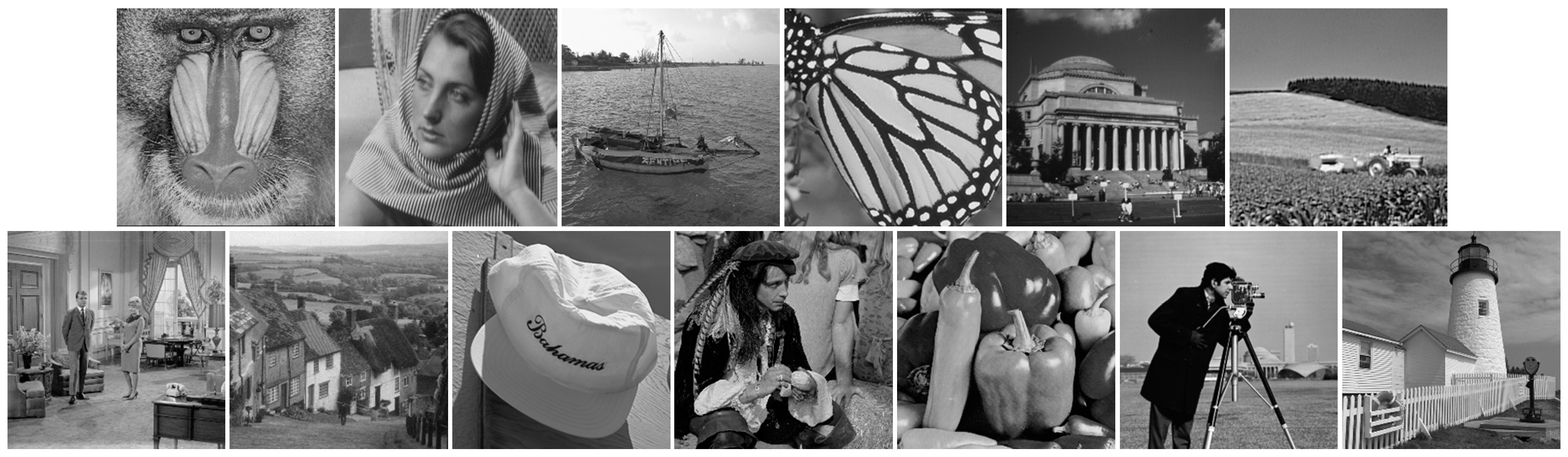
Within the framework of sequential reconstruction, the previously reconstructed pixels will be used in the subsequent pixel reconstruction; hence, the prediction errors will be accumulated and propagated to the later reconstruction. The scan order, which determines the available context of each missing pixel, plays a critical role in the reconstruction performance. A common idea of scan order, as used in [8], is to first reconstruct the missing pixels whose support areas contain more available pixels. Although this scan order has achieved fairly good performance, there are still deficiencies. For example, the scan order will be exactly the same for two different missing areas that have the same area shape. Thus, it is not flexible and conducive for the extension of edges.

In our method, we propose a novel adaptive scan order based on the joint credibility of the support area and reconstruction to alleviate the error propagation problem. The scan order depends not only on the credibility of the support area, but also on the credibility of the missing pixels’ reconstruction. Let $\mathrm{p}(\mathrm{x})$ stand for the confidence of pixel $\mathrm{x}$. Then, the confidences of the pixels in the corrupted image are initialized as:

$$\mathrm{p}(\mathrm{x})=\{\begin{array}{ll}1& \hspace{1em}\mathrm{x} \mathrm{is} \mathrm{the} \mathrm{corresponding} \mathrm{received} \mathrm{pixel}\\ 0& \hspace{1em}\mathrm{x} \mathrm{is} \mathrm{the} \mathrm{missing} \mathrm{pixel}\end{array}$$

(14)

where constant 1 stands for the pixel $\mathrm{x}$ being correctly received, and 0 represents it as missing. We updated the confidence of the missing pixels to 1 after reconstructing them. The confidences of the pixels in the received image were initialized as shown in Figure 10.

For each missing pixel, we find all the possible support areas around it through matching the eight templates. The sum of confidence of all the non-overlapped available pixels in these support areas is used to represent the credibility of the support area of this missing pixel, as shown in the red box in Figure 10. In the process of reconstruction, we firstly reconstructed the missing pixel whose support area had the highest credibility. However, frequently the support areas are the same; as can be seen in Figure 10, the credibility of the support areas of the current pixels ${\mathbf{y}}_1$, ${\mathbf{y}}_2$, ${\mathbf{y}}_3$, and ${\mathbf{y}}_4$ are the same. In this case, we used the credibility of the reconstructions of the current missing pixels to determine the scan order. According to the non-local self-similarity of natural images, similar samples have similar pixel values at the same position. Therefore, we used the deviation between the reconstruction and the pixel value in the same location of the corresponding similar sample to measure the credibility: the lower the deviation, the higher the credibility.

Let ${\mathbf{y}}_i^{\mathrm{u}}$ be the i^th missing pixel that is located on the contour of the available region, and suppose that the n support area ${\mathbf{y}}_i^{{\mathrm{s}}_1},{\mathbf{y}}_i^{{\mathrm{s}}_2},\dots ,{\mathbf{y}}_i^{{\mathrm{s}}_n}$ can be collected through matching the templates. We collected corresponding similar sample sets ${\mathbf{S}}_1,{\mathbf{S}}_2,\dots ,{\mathbf{S}}_n$ from the whole image. Then, the credibility of the reconstruction ${\widehat{\mathbf{y}}}_i^{\mathrm{u}}$ can be represented as:

$$C_i=\frac{1}{\frac{1}{m·n}{\displaystyle \sum _{j=1}^n\sqrt{{\displaystyle \sum _{k=1}^m{({\widehat{\mathbf{y}}}_i^{\mathrm{u}}-{\mathbf{s}}_{j,k}^{\mathrm{u}})}^2}}+\epsilon }}$$

(15)

where ${\widehat{\mathbf{y}}}_i^{\mathrm{u}}$ is the reconstruction of ${\mathbf{y}}_i^{\mathrm{u}}$, and ${\mathbf{s}}_{j,k}^{\mathrm{u}}$ is the true value corresponding to the missing pixel ${\mathbf{y}}_i^{\mathrm{u}}$ in the k^th similar sample of set ${\mathbf{S}}_j$. $\epsilon$ is a constant to ensure that the denominator is not 0. The credibility of the reconstructions of the missing pixels is determined through Formula (15): the higher the credibility, the more reliable the prediction; hence, these missing pixels are reconstructed first.

4. Experiments

In this section, comparative experiments verify the performance of the proposed algorithm. We firstly analyzed the influence of the proposed correction and adaptive scan order to the final EC performance. Then, we compared the proposed method with other state-of-the-art EC methods [4,6,7,9,10,27,31,32] to evaluate our method.

Similar to the work of others, three kinds of block loss were considered in our experiments: a $16\times 16$ regular isolate block losses $\left(\approx 22\% \mathrm{loss} \mathrm{rate}\right)$, $16\times 16$ regular consecutive block losses $\left(\approx 50\% \mathrm{loss} \mathrm{rate}\right)$, and $16\times 16$ random consecutive block losses $\left(\approx 25\% \mathrm{loss} \mathrm{rate}\right)$. This three-loss mode is shown in Figure 11.

For convincing comparisons, 13 widely used images were used as test sets in this paper. Note that we only considered grayscale images; since the color images contain multi-channels, we could reconstruct the color images by reconstructing the channels separately. All of the test images were $256 \times 256$. in size, as illustrated in Figure 12.

In this paper, the size of the designed templates was set to $7\times 7+1$ (that is a combination of a $7\times 7$ square and one pixel to be predicted). The training samples were collected through matching the templates on the test images. Each sample was normalized to the range of [0,1] to serve the active range of ‘tanh’. The two parts of the AE-P network were both 11-layer fully connected networks. We used the ‘elu’ activation function after each layer except for the last layer, and we used the ‘tanh’ activation function after the last layer in order to normalize the output to [0,255], which is the grayscale range. The overview of the AE-P network can be seen in

Table 1. Architectures of the designed AE-P network. After each layer except for the last one we used the ‘elu’ activation function, and after the last layer, we used the ‘tanh’ activation function.

Layer	Number of Neurons
	AE	Prediction
FC 1	49
FC 2	45
FC 3	40
FC 4	35
FC 5	30
FC 6	25
FC 7	30	20
FC 8	35	15
FC 9	40	10
FC 10	45	5
FC 11	49	1

. We used Adam [33] for optimization with the learning rate of the two networks set to 0.001. The batch size was set to 600. In addition, our work is implemented on the Python-Tensorflow platform on Windows 10. The hardware platform used Intel i5 7300H CPU, 8GB of RAM, and NVIDIA GTX 1060 GPU.

In order to compare the quality of reconstruction, the widely used measurement peak signal-to-noise ratio (PSNR) is chosen serve as an objective metric to measure the image quality in our experiments. For a better comparison of structural similarities, the structural similarity (SSIM) index [33] is also used in this paper.

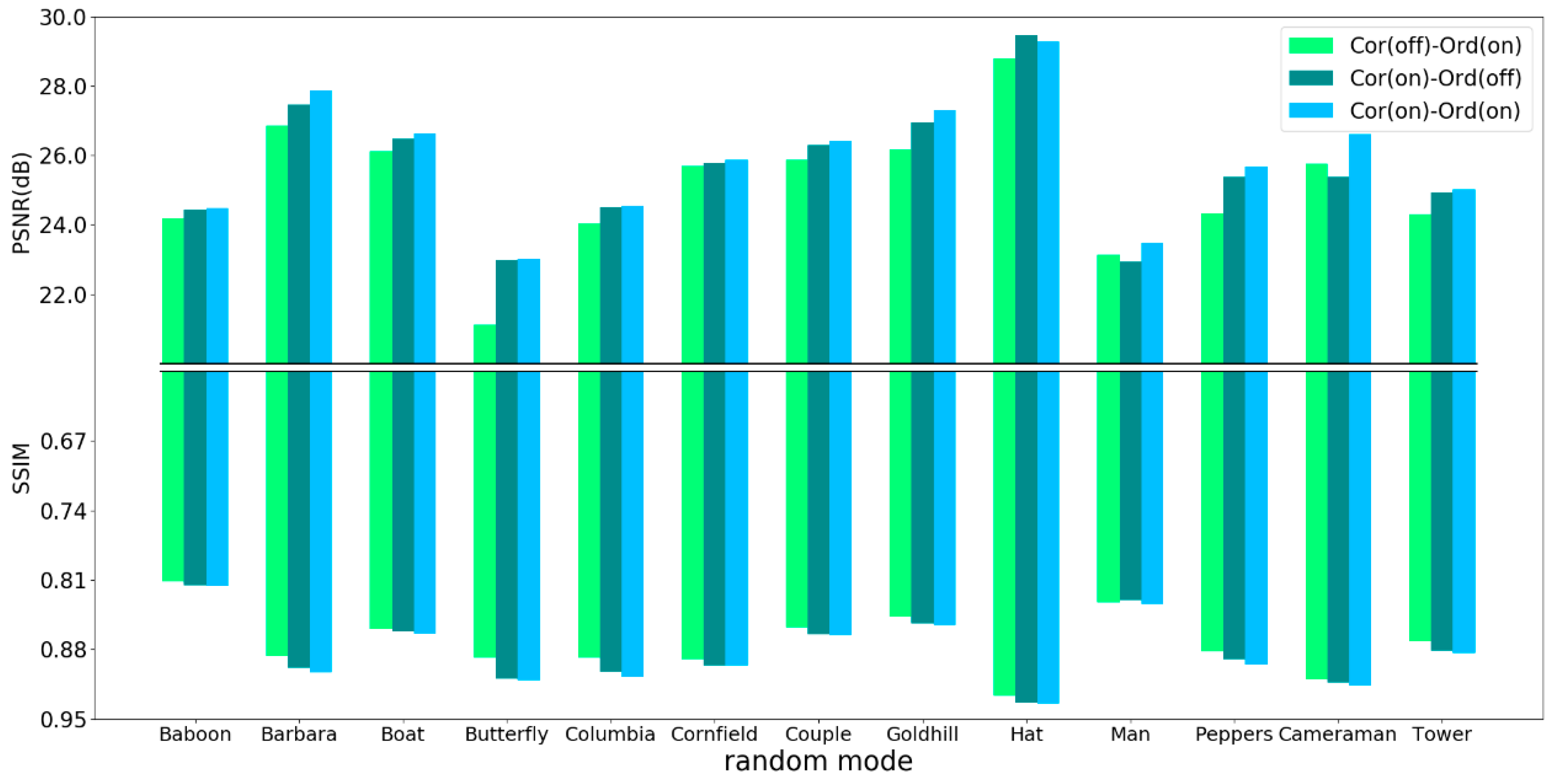
4.1. Comparative Studies

In our method, in order to reduce the prediction error and improve the accuracy of the AE-P network, we corrected the predictions based on the non-local self-similarity of the natural images. Moreover, we proposed an adaptive scan order based on the joint credibility of the support area and reconstruction to alleviate the error propagation problem. To evaluate the influence of the proposed correction and scan order to the final EC performance, we conducted three group comparative experiments corresponding to the three loss modes on the test images. In every group, there were three different scenarios of our method: a scenario that did not use the proposed correction, a scenario that did not use the proposed adaptive scan order, and a scenario that utilized both the proposed correction and the adaptive scan order. For convenience, we named these three scenarios ‘Cor(off)-Ord(on)’, ‘Cor(on)-Ord(off)’, and ‘Cor(on)-Ord(on)’. ‘Cor’ and ‘Ord’ correspond to the proposed correction and scan order, while ‘on’ and ‘off’ in the brackets represent whether they were used or not used. The results of the comparative experiments are shown in Figure 13, Figure 14 and Figure 15.

As can be seen from Figure 13, Figure 14 and Figure 15, in all three loss modes, scenario ‘Cor(on)-Ord(on)’ performed best in almost all of the test images in terms of PSNR and SSIM. In particular, scenario ‘Cor(on)-Ord(on)’ outperformed scenario ‘Cor(off)-Ord(on)’ by a large margin under all the loss modes and test images. The great improvement of reconstruction performance is due to the proposed correction, which can reduce the prediction error effectively. Moreover, it could be observed that the proposed adaptive scan order could also improve the reconstruction performance. Compared with the proposed correction, there is less performance improvement with the scan order. This is because the scan order obtains a better reconstruction performance of the structure, which sometimes produces false edges and leads to the reduction of the PSNR. For example, the scan order fails to improve the reconstruction performance under PSNR in Hat with random loss mode, as shown in Figure 15.

For further evaluation of the influence of the proposed correction and adaptive scan order to the final EC performance, subjective comparisons are given in Figure 16, Figure 17 and Figure 18 corresponding to the three different loss modes. It can be observed that scenario ‘Cor(on)-Ord(on)’ achieved the most comfortable visual and the highest PSNR and SSIM. Specifically, through comparing the method of scenario ‘Cor(off)-Ord(on)’ and the method of scenario ‘Cor(on)-Ord(on)’, we can observe that the proposed correction can greatly improve the reconstruction performance. As shown in the red box in Figure 16c, the bracket inside the red box is disconnected, while the bracket in Figure 16e is connected. We can also observe through the comparison between scenario ‘Cor(on)-Ord(off)’ and scenario ‘Cor(on)-Ord(on)’ that the proposed scan order can improve the reconstruction performance of edges, as shown in the red boxes in Figure 18d,e, respectively.

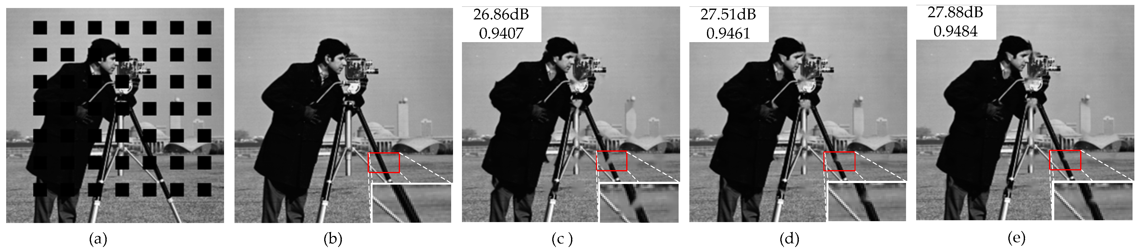
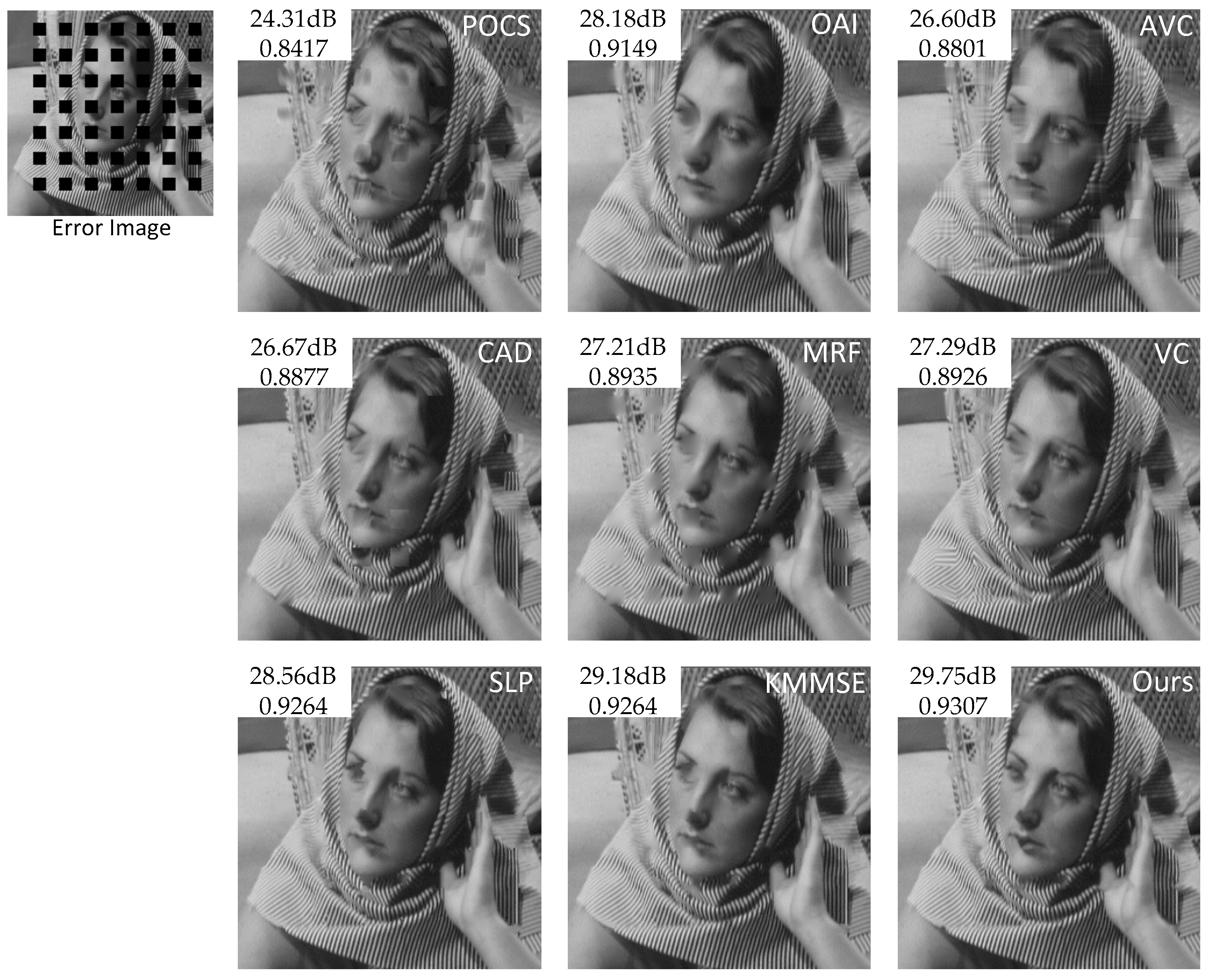
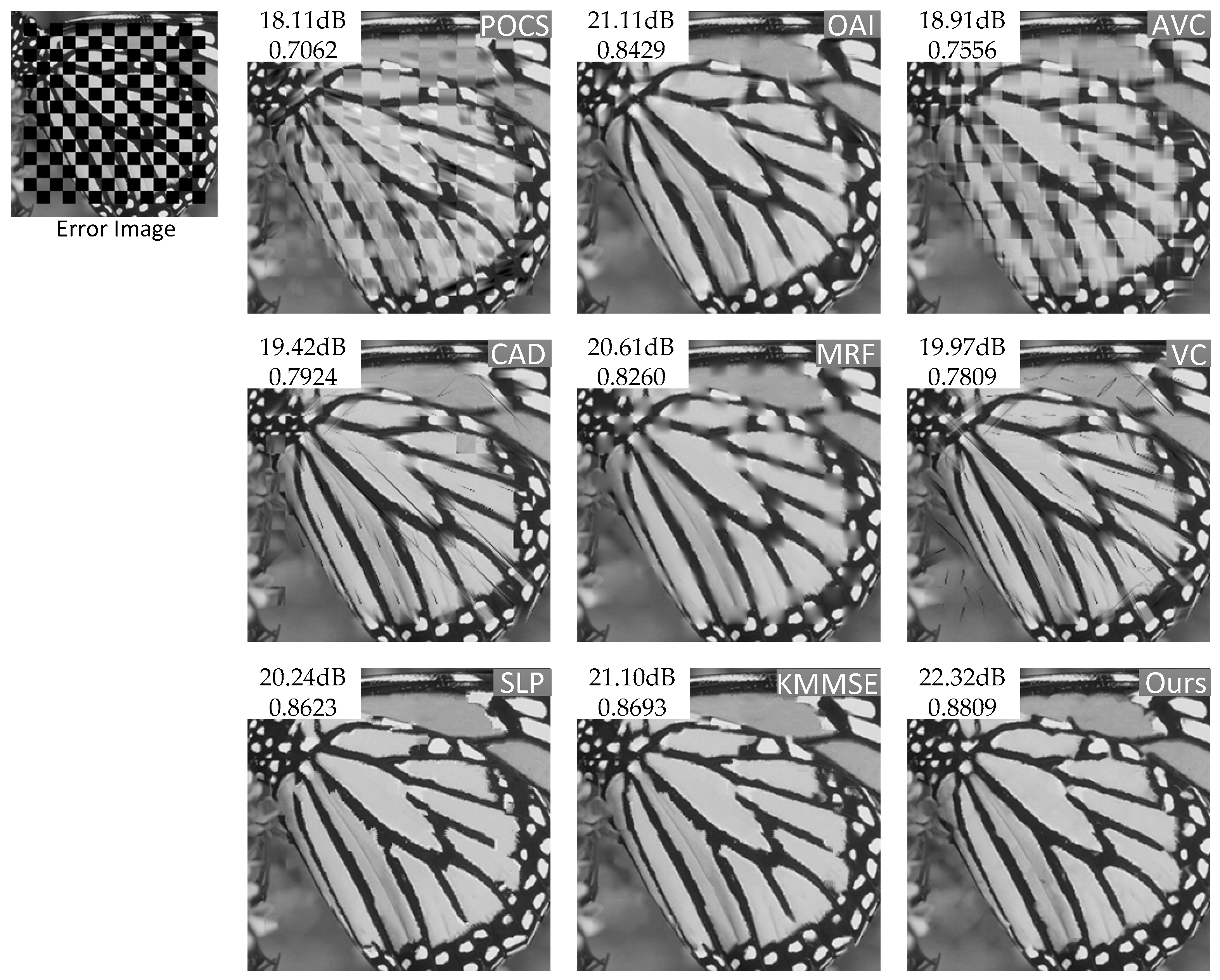
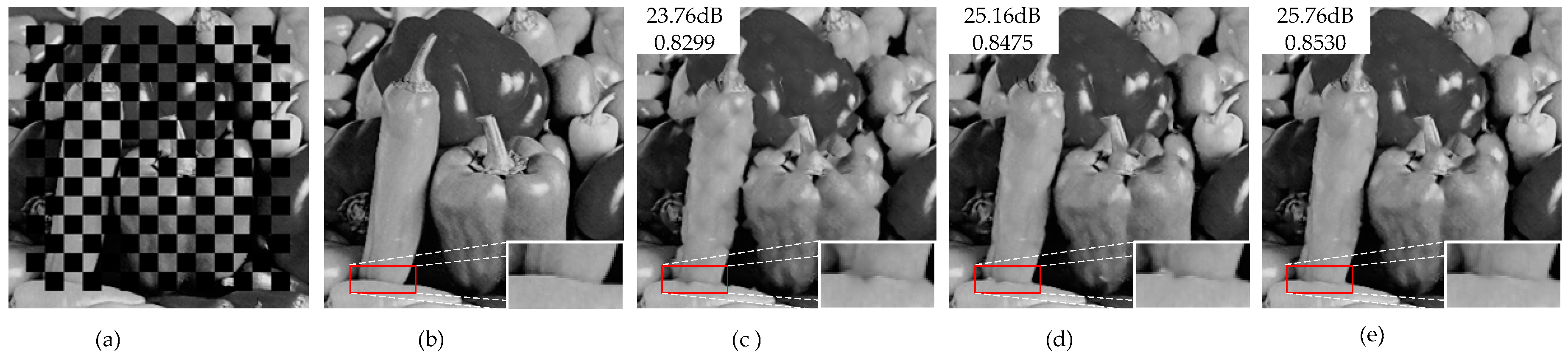
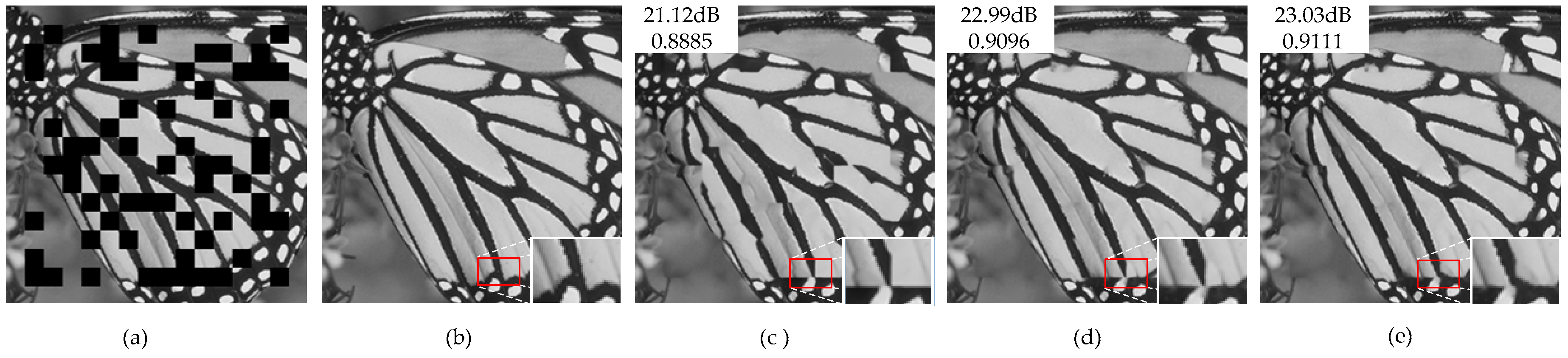
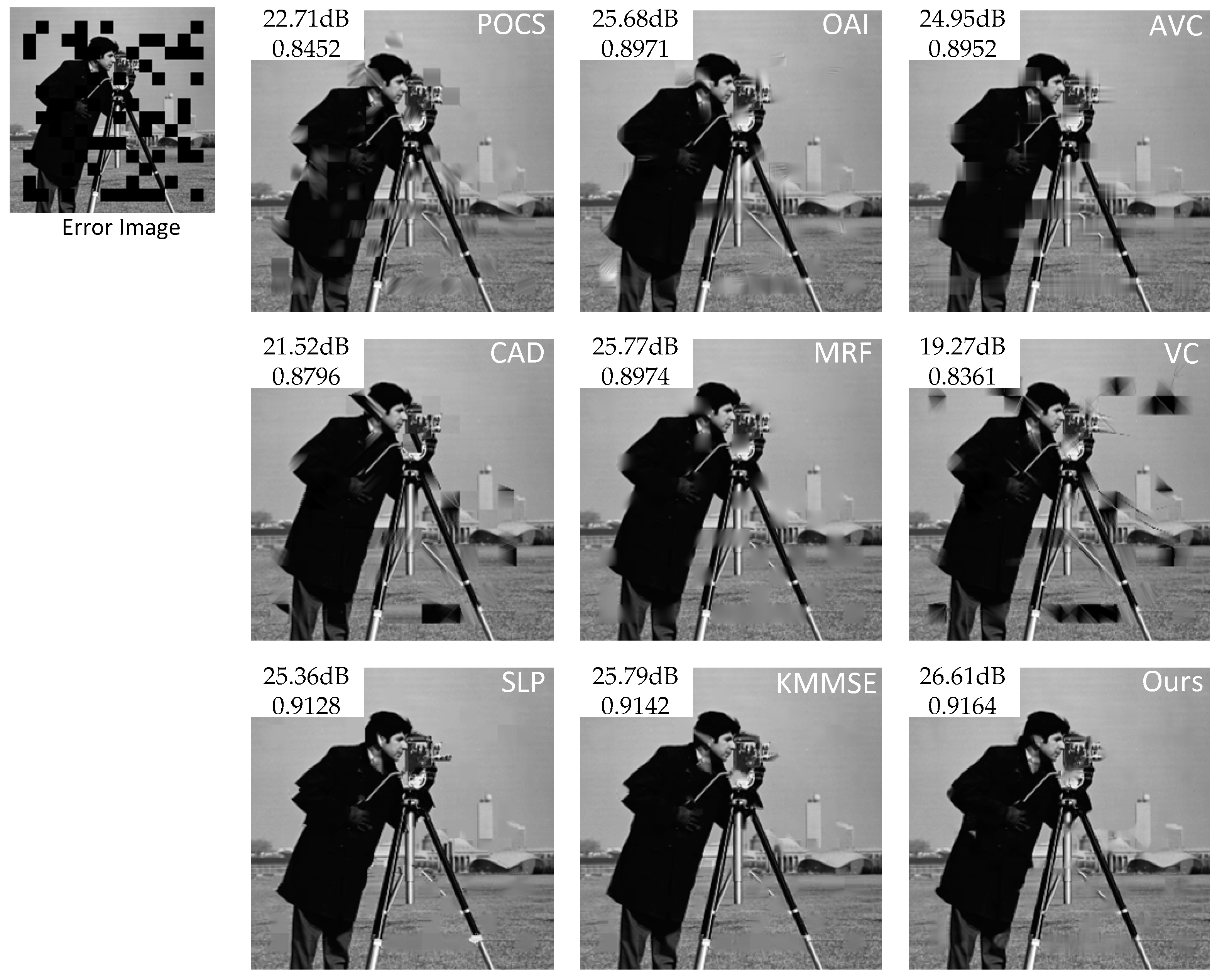
4.2. Objective and Subjective Performance Comparison

In order to verify the performance of the proposed method, eight other state-of-the-art EC methods—POCS [4], MRF [27], nonnormative SEC for H.264 (AVC) [31], content adaptive technique (CAD) [32], OAI [6], VC [7], sparse linear prediction (SLP) [9], and KMMSE [10]—are compared with our method. The source code of all the above methods are based on a third-party implementation [34]. The results of the EC performance comparison of the nine competing methods are given in

Table 2. Peak signal-to-noise ratio (PSNR) and structural similarity (SSIM) index in comparison to EC algorithms with $16\times 16$ regular isolate block losses.

Images	Metrics	Methods
		POCS	OAI	AVC	CAD	MRF	VC	SLP	KMMSE	Ours
Baboon	PSNR	24.58	26.10	25.27	24.36	26.13	25.95	24.60	26.24	26.54
	SSIM	0.8381	0.8678	0.8477	0.8472	0.861	0.8596	0.8573	0.8676	0.8703
Barbara	PSNR	24.31	28.18	26.60	26.67	27.21	27.29	28.56	29.18	29.75
	SSIM	0.8417	0.9149	0.8801	0.8877	0.8935	0.8926	0.9254	0.9264	0.9311
Boat	PSNR	26.50	27.53	27.29	26.07	27.10	27.12	26.44	27.49	27.65
	SSIM	0.8723	0.8964	0.8893	0.8815	0.7781	0.8913	0.8893	0.8938	0.8958
Butterfly	PSNR	20.56	25.10	21.91	23.07	23.72	24.19	24.21	24.46	26.34
	SSIM	0.8599	0.9251	0.8755	0.9221	0.9090	0.9280	0.9426	0.9440	0.9474
Columbia	PSNR	23.76	26.46	25.07	25.84	25.45	27.46	26.36	26.94	28.02
	SSIM	0.8859	0.9338	0.9229	0.9272	0.9160	0.9288	0.9404	0.9395	0.9429
Cornfield	PSNR	26.69	28.97	28.88	26.62	28.50	28.97	28.36	29.19	30.42
	SSIM	0.8954	0.9318	0.9269	0.9201	0.9027	0.9303	0.9326	0.9371	0.9422
Couple	PSNR	25.08	27.87	27.44	26.10	27.42	27.56	27.13	27.84	28.04
	SSIM	0.8590	0.9071	0.8932	0.8841	0.8915	0.8980	0.9010	0.9044	0.9073
Goldhill	PSNR	26.40	28.50	28.24	25.06	27.95	28.38	28.21	28.78	28.82
	SSIM	0.8612	0.8975	0.8877	0.8624	0.8856	0.8909	0.8948	0.8978	0.8997
Hat	PSNR	27.28	31.63	28.72	29.74	30.35	31.04	31.20	31.82	32.56
	SSIM	0.8994	0.9501	0.9315	0.9431	0.9442	0.9427	0.9522	0.9576	0.9636
Man	PSNR	23.14	26.35	24.83	24.30	25.46	25.72	24.06	25.68	25.54
	SSIM	0.8350	0.8843	0.8613	0.847	0.8748	0.8727	0.8758	0.8845	0.8799
Peppers	PSNR	24.29	29.93	27.37	27.92	28.46	28.85	29.08	29.50	29.98
	SSIM	0.8584	0.9293	0.9062	0.9098	0.9229	0.9164	0.9294	0.9300	0.9306
Cameraman	PSNR	23.89	27.55	26.29	26.96	26.84	26.83	26.31	27.37	27.88
	SSIM	0.8858	0.9402	0.9290	0.9332	0.9298	0.9327	0.9464	0.9482	0.9484
Tower	PSNR	23.68	26.78	26.13	25.36	25.17	26.53	25.71	26.50	27.15
	SSIM	0.8801	0.9197	0.9089	0.9093	0.9080	0.9175	0.9191	0.9262	0.9279
Average	PSNR	24.63	27.77	26.46	26.01	26.90	27.38	26.94	27.77	28.36
	SSIM	0.8671	0.9152	0.8969	0.8981	0.8936	0.9078	0.9159	0.9198	0.9221

,

Table 3. PSNR and SSIM comparison of EC algorithms with $16\times 16$ regular consecutive block losses.

Images	Metrics	Methods
		POCS	OAI	AVC	CAD	MRF	VC	SLP	KMMSE	Ours
Baboon	PSNR	21.38	22.77	22.27	19.81	22.94	21.76	21.26	22.92	22.95
	SSIM	0.6719	0.7305	0.6981	0.6554	0.7202	0.6872	0.7013	0.7228	0.7208
Barbara	PSNR	21.32	25.19	23.36	22.16	24.23	22.65	25.36	26.59	26.53
	SSIM	0.6993	0.8407	0.7693	0.772	0.8019	0.7531	0.8520	0.8620	0.8593
Boat	PSNR	23.89	24.14	24.83	22.59	24.80	23.32	23.46	24.53	24.93
	SSIM	0.7427	0.7942	0.7892	0.7613	0.7781	0.7376	0.7716	0.7833	0.7951
Butterfly	PSNR	18.11	21.11	18.91	19.42	20.61	19.97	20.24	21.10	22.77
	SSIM	0.7062	0.8429	0.7556	0.7925	0.8260	0.7809	0.8623	0.8693	0.8814
Columbia	PSNR	21.66	24.17	22.91	23.74	23.48	24.12	23.35	24.23	25.05
	SSIM	0.7722	0.8679	0.8454	0.8537	0.8280	0.8172	0.8600	0.8665	0.8655
Cornfield	PSNR	23.84	24.88	25.31	23.07	25.12	24.35	24.13	25.27	25.66
	SSIM	0.7927	0.8624	0.8563	0.8172	0.8393	0.7859	0.8492	0.8617	0.8651
Couple	PSNR	21.95	24.62	23.96	22.17	23.55	22.94	22.56	23.54	24.76
	SSIM	0.7191	0.8118	0.782	0.773	0.7747	0.7510	0.7748	0.7886	0.7940
Goldhill	PSNR	23.61	25.37	25.44	23.50	25.24	24.69	24.75	25.43	25.62
	SSIM	0.7321	0.7995	0.7818	0.7489	0.7785	0.7594	0.7822	0.7908	0.7920
Hat	PSNR	24.52	28.40	26.27	24.18	27.57	25.17	27.31	27.73	28.62
	SSIM	0.7947	0.8913	0.8606	0.8128	0.8844	0.7931	0.8954	0.8998	0.9010
Man	PSNR	19.77	22.14	21.77	17.17	22.13	21.60	21.02	22.06	22.49
	SSIM	0.6668	0.7501	0.72	0.6701	0.7390	0.7085	0.7310	0.7461	0.7542
Peppers	PSNR	20.88	25.73	23.16	19.71	24.14	23.18	23.52	24.14	25.76
	SSIM	0.7209	0.8516	0.8055	0.7696	0.8319	0.7770	0.8371	0.8434	0.8530
Cameraman	PSNR	20.42	24.06	22.41	20.42	22.62	22.51	22.63	23.16	23.74
	SSIM	0.7654	0.8704	0.8417	0.8333	0.8475	0.7941	0.8753	0.8757	0.8747
Tower	PSNR	20.37	23.47	22.78	21.04	22.04	22.55	22.47	23.35	23.96
	SSIM	0.7499	0.8339	0.8106	0.7826	0.8030	0.7704	0.8311	0.8407	0.8354
Average	PSNR	21.67	24.31	23.34	21.46	23.73	22.99	23.24	24.16	24.83
	SSIM	0.7334	0.8267	0.7935	0.7725	0.8040	0.7627	0.8172	0.8270	0.8301

and

Table 4. PSNR and SSIM comparison of EC algorithms with $16\times 16$ random consecutive block losses.

Images	Metrics	Methods
		POCS	OAI	AVC	CAD	MRF	VC	SLP	KMMSE	Ours
Baboon	PSNR	22.93	23.72	23.81	20.44	24.38	18.93	22.76	24.20	24.47
	SSIM	0.7852	0.8142	0.7986	0.7801	0.8125	0.7837	0.8049	0.8146	0.8163
Barbara	PSNR	22.92	25.80	25.07	21.62	25.85	19.91	26.76	27.77	27.77
	SSIM	0.7995	0.8747	0.8445	0.8327	0.8621	0.8235	0.8959	0.8997	0.9033
Boat	PSNR	25.37	26.08	26.44	21.85	26.38	18.01	25.11	26.17	26.64
	SSIM	0.8336	0.8611	0.8601	0.825	0.8590	0.8089	0.8564	0.8635	0.8637
Butterfly	PSNR	19.27	21.96	19.93	18.49	21.58	17.93	21.54	22.05	23.03
	SSIM	0.8031	0.8754	0.827	0.8484	0.8739	0.8422	0.9038	0.9008	0.9111
Columbia	PSNR	22.26	23.77	22.86	22.59	23.10	21.80	23.79	24.25	24.54
	SSIM	0.8463	0.8898	0.8875	0.8806	0.8757	0.8537	0.8990	0.9063	0.9077
Cornfield	PSNR	25.23	25.04	26.33	21.32	26.05	19.42	25.51	26.48	25.87
	SSIM	0.8555	0.8869	0.8948	0.8591	0.8785	0.8263	0.8930	0.9004	0.8963
Couple	PSNR	23.60	25.45	25.66	22.06	25.42	19.77	24.15	25.31	26.40
	SSIM	0.8125	0.8571	0.8544	0.8281	0.8505	0.8214	0.8520	0.8574	0.8656
Goldhill	PSNR	25.16	26.61	27.13	22.70	27.12	20.81	26.76	27.51	27.31
	SSIM	0.8177	0.8546	0.8498	0.8069	0.8460	0.8102	0.8574	0.8608	0.8552
Hat	PSNR	26.18	27.83	26.98	21.36	28.42	19.5802	27.50	29.15	29.28
	SSIM	0.8763	0.9076	0.9081	0.8661	0.9278	0.8344	0.9294	0.9386	0.9346
Man	PSNR	21.39	23.17	22.36	20.49	22.77	21.2781	21.71	22.76	23.48
	SSIM	0.7783	0.8308	0.8125	0.7793	0.8249	0.8096	0.8211	0.8315	0.8346
Peppers	PSNR	21.66	25.41	23.28	21.35	24.05	20.09	24.75	25.06	25.67
	SSIM	0.8163	0.8772	0.8542	0.836	0.8733	0.8284	0.8892	0.8925	0.8955
Cameraman	PSNR	22.71	25.68	24.95	21.51	25.77	19.27	25.36	25.79	26.61
	SSIM	0.8452	0.8971	0.8952	0.8796	0.8974	0.8361	0.9128	0.9142	0.9164
Tower	PSNR	22.22	23.99	24.35	21.81	23.44	19.84	24.85	25.44	25.01
	SSIM	0.8276	0.8704	0.869	0.854	0.8626	0.8321	0.8854	0.8918	0.8834
Average	PSNR	23.15	24.96	24.55	21.35	24.95	19.74	24.66	25.53	25.85
	SSIM	0.8229	0.8690	0.8581	0.8366	0.8649	0.8239	0.8769	0.8825	0.8834

. As can be seen from the tables, our method is superior to the other eight methods in average PSNR and SSIM under three loss modes.

Table 2 illustrates the reconstruction performance of the compared methods on $16 \times 16$ isolate block losses. As can be observed from Table 2, the proposed method outperformed all of the other methods in average PSNR by a considerable margin. Compared with the very recent image EC method KMMSE, the average PSNR gain was 0.59 dB. Compared with the well-known OAI method, our method achieved up to 0.59 dB higher PSNR and 0.0069 higher SSIM. When compared with the POCS, VC, SLP, and MRF methods, our method obtained gains of 3.73 dB, 0.98 dB, 1.42 dB, and 1.46 dB in terms of PSNR and gains of 0.0550, 0.0143, 0.0062, and 0.0285 in terms of SSIM, respectively.

Table 3 shows the quantitative comparison of $16\times 16$ regular consecutive block losses. Under this loss mode, the proposed method performed better than the remaining eight methods on all of the test images in terms of both PSNR and SSIM. The average performance over the second-best method was over 0.52 dB in terms of PSNR and 0.0034 in terms of SSIM. Similarly, compared with the POCS, VC, SLP, and MRF methods, our method obtained gains of 3.16 dB, 1.84 dB, 1.59 dB, and 1.1 dB in terms of PSNR and gains of 0.0967, 0.0674, 0.0129, and 0.0261 in terms of SSIM, respectively. Moreover, compared with the recent image EC method KMMSE, the average PSNR gain is 0.67 dB.

Finally, we compared the reconstruction quality of our method with the other methods on random consecutive block losses. As illustrated in Table 4, the proposed method gained the best performance under the average PSNR and SSIM. Specifically, compared with KMMSE, SLP, and AVC, the average PSNR gains were 0.32 dB, 1.19 dB, and 1.3 dB, respectively.

In order to represent the performance of the proposed method, subjective comparisons are also given in Figure 19, Figure 20 and Figure 21. As can be observed from the figures, the proposed method produced the most visually pleasant results among all compared methods. Figure 19 compares the performance of the proposed method with the others working under isolate block loss. Severe blocking artifacts were produced in POCS, AVC, CAD and VC, and a blurred and lumpy boundary could be observed in MRF and OAI. Figure 20 presents the comparison results on regular consecutive block losses, which has the high block loss rate. The POCS, CAD, and MRF produced very serious lumps. It also observed that the CAD and VC methods produced many false edges. Only the proposed method and the recent KMMSE method produced a natural reconstruction. Figure 21 presents the comparison results on random block losses; under this loss mode, the EC task is more challenging since many missing blocks may cluster together, making it difficult to find a regular and reliable neighborhood. It can be found that some loss pixels cannot be estimated very well. Only the proposed method can restore the major edges and textures.

Regarding the run time of our proposal, since we needed to train an AE-P network for each corrupted image, the training time of the network was included in the entire image processing time. In addition, the algorithm that we implemented is not optimized; for example, we used an exhaustive search to collect similar samples. These two reasons made our algorithm time-intensive. More specifically, our algorithm required about half an hour per corrupted image under 16 $\times$ 16 isolate loss mode and a 256 $\times$ 256 image size. Therefore, our algorithm is computationally prohibitive for online applications. Although the proposed algorithm requires a longer time than the compared method, the reconstruction quality of our method is better than the others in terms of average PSNR and SSIM, as shown in Table 2, Table 3 and Table 4. Therefore, our future works will improve our algorithm in two ways. One is to optimize the algorithm and reduce the computational complexity. The other is to use a pre-trained network to avoid training the network for each image.

5. Conclusions

In this paper, we developed a novel image EC method based on the AE-P neural network. Both the local correlation and non-local self-similarity of natural images were taken into account in reconstructing the missing pixels. We used the local correlation to predict the missing pixels and the non-local information to correct the predictions. The designed neural network could be divided into two parts: the prediction part and the auto-encoder (AE) part. The prediction part utilized the local correlation among pixels to predict the missing ones. The AE part extracted image features, which were used to collect similar samples from the whole image. The predictions of the missing pixels were corrected through the collected similar samples. In addition, we proposed a novel adaptive scan order based on the joint credibility of the support area and reconstruction to alleviate the error propagation problem. The experimental results showed that the proposed algorithm could reconstruct corrupted images effectively and outperform the compared state-of-the-art methods in terms of objective and perceptual metrics.

References

1. Zhang, Y.; Xiang, X.; Zhao, D.; Ma, S.; Gao, W. Packet video error concealment with auto regressive model. IEEE Trans. Circuits Syst. Video Technol. 2012, 1, 12–27. [Google Scholar] [CrossRef]
2. Zhai, G.; Yang, X.; Lin, W.; Zhang, W. Bayesian error concealment with DCT pyramid for images. IEEE Trans. Circuits Syst. Video Technol. 2010, 9, 1224–1232. [Google Scholar] [CrossRef]
3. Hsia, S.C. An edge-oriented spatial interpolation for consecutive block error concealment. IEEE Signal Process. Lett. 2004, 1, 577–580. [Google Scholar] [CrossRef]
4. Sun, H.; Kwok, W. Concealment of damaged block transform coded images using projections onto convex sets. IEEE Trans. Image Process. 1995, 4, 470–477. [Google Scholar] [CrossRef] [PubMed]
5. Zeng, W.; Liu, B. Geometric-structure-based error concealment with novel applications in block-based low-bit-rate coding. IEEE Trans. Circuits Syst. Video Technol. 1999, 1, 648–665. [Google Scholar] [CrossRef]
6. Li, X.; Orchard, M.T. Novel sequential error-concealment techniques using orientation adaptive interpolation. IEEE Trans. Circuits Syst. Video Technol. 2002, 10, 857–864. [Google Scholar]
7. Koloda, J.; Sánchez, V.; Peinado, A.M. Spatial Error Concealment Based on Edge Visual Clearness for Image/Video Communication. Circuits Syst. Signal Process. 2013, 4, 815–824. [Google Scholar] [CrossRef]
8. Liu, J.; Zhai, G.; Yang, X.; Yang, B.; Chen, L. Spatial error concealment with an adaptive linear predictor. IEEE Trans. Circuits Syst. Video Technol. 2015, 3, 353–366. [Google Scholar]
9. Koloda, J.; Ostergaard, J.; Jensen, S.H.; Sánchez, V.; Peinado, A.M. Sequential error concealment for video/images by sparse linear prediction. IEEE Trans. Multimed. 2013, 6, 957–969. [Google Scholar] [CrossRef]
10. Koloda, J.; Peinado, A.M.; Sánchez, V. Kernel-based MMSE multimedia signal reconstruction and its application to spatial error concealment. IEEE Trans. Multimed. 2014, 10, 1729–1738. [Google Scholar] [CrossRef]
11. Park, J.; Park, D.C.; Marks, R.J.; El-Sharkawi, M.A. Recovery of image blocks using the method of alternating projections. IEEE Trans. Image Process. 2005, 4, 461–474. [Google Scholar] [CrossRef]
12. Koloda, J.; Seiler, J.; Peinado, A.M.; Kaup, A. Scalable kernel-based minimum mean square error estimator for accelerated image error concealment. IEEE Trans. Broadcast. 2017, 11, 59–70. [Google Scholar] [CrossRef]
13. Akbari, A.; Trocan, M.; Granard, B. Joint-domin dictionary learning-based error concealment using common space mapping. In Proceedings of the 2017 22nd International Conference on Digital Signal Processing-DSP, London, UK, 23–25 August 2017; pp. 1–5. [Google Scholar]
14. Ding, D.; Ram, S.; Rodríguez, J.J. Image inpainting using nonlocal texture matching and nonlinear filtering. IEEE Trans. Image Process. 2019, 4, 1705–1719. [Google Scholar] [CrossRef]
15. Alilou, V.K.; Yaghmaee, F. Application of GRNN neural network in non-texture image inpainting and restoration. Pattern Recognit. Lett. 2015, 9, 24–31. [Google Scholar] [CrossRef]
16. Lam, W.M.; Reibman, A.R.; Liu, B. Recovery of lost or erroneously received motion vectors. In Proceedings of the 1993 IEEE International Conference on Acoustics, Speech, and Signal Processing-ICASSP, Minneapolis, MN, USA, 27–30 April 1993; Volume 5, pp. 417–420. [Google Scholar]
17. Zhang, J.; Arnold, J.F.; Frater, M.R. A cell-loss concealment technique for MPEG-2 coded video. IEEE Trans. Circuits Syst. Video Technol. 2000, 6, 659–665. [Google Scholar] [CrossRef]
18. Wu, J.; Liu, X.; Yoo, K.Y. A temporal error concealment method for H.264/AVC using motion vector recovery. IEEE Trans. Consum. Electron. 2008, 11, 1880–1885. [Google Scholar] [CrossRef]
19. Qian, X.; Liu, G.; Wang, W. Recovering connected error region based on adaptive error concealment order determination. IEEE Trans. Multimed. 2009, 6, 683–695. [Google Scholar] [CrossRef]
20. Shao, S.C.; Chen, J.H. A novel error concealment approach based on general regression neural network. In Proceedings of the 2011 International Conference on Consumer Electrics, Communication and Networks-CECNet, XianNing, China, 16–18 April 2011; pp. 4679–4682. [Google Scholar]
21. Sankisa, A.; Punjabi, A.; Katsaggelos, A.K. Video error concealment using deep neural networks. In Proceedings of the IEEE International Conference on Image Processing-ICIP, Athens, Greece, 7–10 October 2018; pp. 380–384. [Google Scholar]
22. Ghuge, A.D.; Rajani, P.K.; Khaparde, A. Video error concealment using moment Invariance. In Proceedings of the 2017 International Conference on Computing, Communication, Control and Automation-ICCUBEA, Pune, India, 17–18 August 2017; pp. 1–5. [Google Scholar]
23. Zhang, Y.; Xiang, X.; Ma, S.; Zhao, D.; Gao, W. Auto regressive model and weighted least squares based packet video error concealment. In Proceedings of the 2010 Data Compression Conference-DCC, Snowbird, UT, USA, 24–26 March 2010; pp. 455–464. [Google Scholar]
24. Agrafiotis, D.; Bull, D.R.; Canagarajah, C.N. Enhanced error concealment with mode selection. IEEE Trans. Circuits Syst. Video Technol. 2006, 8, 960–973. [Google Scholar] [CrossRef]
25. Kung, W.-Y.; Kim, C.-S.; Kuo, C.-C.J. Spatial and temporal error concealment techniques for video transmission over noisy channels. IEEE Trans. Circuits Syst. Video Technol. 2006, 7, 789–803. [Google Scholar] [CrossRef]
26. Ma, M.; Au, O.C.; Chan, S.-H.G.; Sun, M.-T. Edge-directed error concealment. IEEE Trans. Circuits Syst. Video Technol. 2010, 3, 382–395. [Google Scholar]
27. Shirani, S.; Kossentini, F.; Ward, R. An Adaptive Markov Random Field Based Error Concealment Method for Video Communication in an Error Prone Environment. In Proceedings of the 1999 IEEE International Conference on Acoustics, Speech, and Signal Processing-ICASSP, Phoenix, AZ, USA, 15–19 March 1999; Volume 6, pp. 3117–3120. [Google Scholar]
28. Koloda, J.; Peinado, A.M.; Sánchez, V. On the application of multivariate kernel density estimation to image error concealment. In Proceedings of the 2013 IEEE International Conference on Acoustics, Speech, and Signal Processing-ICASSP, Vancouver, BC, Canada, 26–31 May 2013; pp. 1330–1334. [Google Scholar]
29. Liu, X.; Zhai, D.; Zhou, J.; Wang, S. Sparsity-Based image error concealment via adaptive dual dictionary learning and regularization. IEEE Trans. Image Process. 2017, 2, 782–796. [Google Scholar] [CrossRef] [PubMed]
30. Hinton, G.E.; Salakhutdinov, R.R. Reducing the Dimensionality of Data with Neural Networks. Science 2006, 7, 504–507. [Google Scholar] [CrossRef] [PubMed]
31. Varsa, V.; Hannuksela, M.M.; Wang, Y.-K. Non-Normative Error Concealment Algorithms. In Proceedings of the 14th ITU-T VCEG Meeting Document: VCEG-N62, Santa Barbara, CA, USA, 21–24 September 2001. [Google Scholar]
32. Rongfu, Z.; Yuanhua, Z.; Xiaodong, H. Content-adaptive spatial error concealment for video communication. IEEE Trans. Consum. Electron. 2004, 2, 335–341. [Google Scholar] [CrossRef]
33. Wang, Z.; Bovik, A.C.; Sheikh, H.R.; Simoncelli, E.P. Image quality assessment: From error visibility to structural similarity. IEEE Trans. Image Process. 2004, 4, 600–612. [Google Scholar] [CrossRef]
34. Janko. Available online: http://dtstc.ugr.es/~jkoloda/download.html (accessed on 1 March 2019).
Figure 1. Structure of the corrupted image. Each square stands for one pixel. The black pixels are unavailable ones. The white pixels are correctly received ones. The pixel being predicted is marked in red, and the pixels marked blue are the pixels corresponding to the current pixel y i u of the similar samples.
Algorithms 12 00082 g001
Figure 2. Block diagram of the proposed method. The missing pixel y i u is under process. The square patches t i ( i = 1 , 2 , , n ) are the collected samples for training. The square patches s i ( i = 1 , 2 , , m ) are the samples that are similar to the current support area y i s .
Algorithms 12 00082 g002
Figure 3. Structure of the utilized neural networks. (a) The structure of auto-encoder part network. (b) The structure of the prediction part network.
Algorithms 12 00082 g003
Figure 4. Structure of the designed auto-encoder prediction (AE-P) network.
Algorithms 12 00082 g004
Figure 5. The red square is the current missing pixel, the gray squares are the available pixels, and the black squares are the unavailable pixels. (a) The template with square shape. (b) The context of the current missing pixel through matching the square template.
Algorithms 12 00082 g005
Figure 6. The eight different templates used in our method. The black squares stand for the missing pixels, and the white squares are the successfully received ones.
Algorithms 12 00082 g006
Figure 7. The red square stands for the current missing pixel. Four support area can be found for the currently missing pixel.
Algorithms 12 00082 g007
Figure 8. The procedure of transforming the shape from up-left into the standard shape down-left.
Algorithms 12 00082 g008
Figure 9. Structure of the augmented samples for selecting in pixel space. Each square stands for one pixel. The green part are the added pixels.
Algorithms 12 00082 g009
Figure 10. The initialization confidence of pixels in the received image. Each square stands for one pixel. The gray pixels with label 1 represent the correctly received pixels, while the green ones with label 0 are the missing pixels. The red pixels are the currently being filled. The part in the red box is the support areas of the missing pixel y 1 .
Algorithms 12 00082 g010
Figure 11. Typical block loss mode. (a) Isolate block loss. (b) Consecutive block loss. (c) Random block loss.
Algorithms 12 00082 g011
Figure 12. The 13 test images used in our experiments. From left to right and top to bottom: Baboon, Barbara, Boat, Butterfly, Columbia, Cornfield, Couple, Goldhill, Hat, Man, Peppers, Tower.
Algorithms 12 00082 g012
Figure 13. The influence of the proposed correction and adaptive scan order to the final error concealment (EC) performance under the 16 × 16 regular isolated loss mode.
Algorithms 12 00082 g013
Figure 14. The influence of the proposed correction and adaptive scan order to the final EC performance under the 16 × 16 regular consecutive loss mode.
Algorithms 12 00082 g014
Figure 15. The influence of the proposed correction and adaptive scan order to the final EC performance under the 16 × 16 random loss mode.
Algorithms 12 00082 g015
Figure 16. Subjective quality comparison of the proposed correction and adaptive scan order on the Cameraman image with 16 × 16 regular isolated loss. The reconstructed details are shown in the lower right corner of each image. (a) The received image. (b) The original image. (c) The reconstructed image with scenario ‘Cor(off)-Ord(on)’. (d) The reconstructed image with scenario ‘Cor(on)-Ord(off)’. (e) The reconstructed image with scenario ‘Cor(on)-Ord(on)’.
Algorithms 12 00082 g016
Figure 17. Subjective quality comparison of the proposed correction and adaptive scan order on the Peppers image with 16 × 16 regular consecutive loss. The reconstructed details are shown in the lower right corner of each image. (a) The received image. (b) The original image. (c) The reconstructed image with scenario ‘Cor(off)-Ord(on)’. (d) The reconstructed image with scenario ‘Cor(on)-Ord(off)’. (e) The reconstructed image with scenario ‘Cor(on)-Ord(on)’.
Algorithms 12 00082 g017
Figure 18. Subjective quality comparison of the proposed correction and adaptive scan order on the Butterfly image with 16 × 16 random loss. The reconstructed details are shown in the lower right corner of each image. (a) The received image. (b) The original image. (c) The reconstructed image with scenario ‘Cor(off)-Ord(on)’. (d) The reconstructed image with scenario ‘Cor(on)-Ord(off)’. (e) The reconstructed image with scenario ‘Cor(on)-Ord(on)’.
Algorithms 12 00082 g018
Figure 19. Subjective comparison of different EC algorithms on the Barbara image with 16 × 16 isolate block loss. The corresponding PSNR and SSIM values are also shown in the upper left corner.
Algorithms 12 00082 g019
Figure 20. Subjective comparison of different EC algorithms on the Butterfly image with 16 × 16 consecutive block loss. The corresponding PSNR and SSIM values are also shown in the upper left corner.
Algorithms 12 00082 g020
Figure 21. Subjective comparison of different EC algorithms on the Cameraman image with 16 × 16 random block loss. The corresponding PSNR and SSIM values are also shown in the upper left corner.
Algorithms 12 00082 g021