Direct Superbubble Detection

Abstract

Superbubbles are a class of induced subgraphs in digraphs that play an essential role in assembly algorithms for high-throughput sequencing data. They are connected with the remainder of the host digraph by a single entrance and a single exit vertex. Linear-time algorithms for the enumeration superbubbles recently have become available. Current approaches require the decomposition of the input digraph into strongly-connected components, which are then analyzed separately. In principle, a single depth-first search could be used, provided one can guarantee that the root of the depth-first search (DFS)-tree is not itself located in the interior or the exit point of a superbubble. Here, we describe a linear-time algorithm to determine suitable roots for a DFS-forest that is guaranteed to identify the superbubbles in a digraph correctly. In addition to the advantages of a more straightforward implementation, we observe a nearly three-fold gain in performance on real-world datasets. We present a reference implementation of the new algorithm that accepts many commonly-used input formats for digraphs. It is available as open source from github.

1. Introduction

Bubble structures in a digraph have become the focus of an increasing body of research because of their role in genome assembly and related topics; see, e.g., [1] and the references therein. Onodera et al. [2] proposed superbubbles as an important class of subgraphs in the de Bruijn and overlap digraphs arising in the context of the assembly of high-throughput sequencing data [3,4]. The algorithm identifying all superbubbles in a digraph G with vertex set V and edge set $\left|E\right|$ had a running time $O\left(\right|V\left|\right(\left|V\right|+\left|E\right|\left)\right)$ [2]. An improvement to $O\left(\right|E|log|E\left|\right)$ was described in [5]. A linear time algorithm for an acyclic subgraph together with the construction of auxiliary digraphs along the lines of [5] provided a solution in $O\left(\right|E|+|V\left|\right)$, i.e., linear, overall time [6]. An alternative linear-time algorithm [7] achieves a substantial speedup and does not require sophisticated data structures. All these approaches rely on the decomposition of G into its strongly-connected components and require the construction of intermediate auxiliary digraphs. Here, we show that the subdivision of the problem, as well as the construction of auxiliary digraphs, can be avoided. This additional simplification yields a further performance gain.

2. Theory

2.1. Oriented Trees and DFS-trees

A directed graph (digraph) G consists of a vertex set $V=V\left(G\right)$ and a set $E=E\left(G\right)$ of directed edges such that $(u,v)\in E\left(G\right)$ implies $u,v\in V\left(G\right)$. H is a sub-digraph of G if $V\left(H\right)\subseteq V\left(G\right)$ and $E\left(H\right)\subseteq E\left(G\right)$. $G\left[W\right]$ is the subgraph induced by W if $V\left(G\right[W\left]\right)=W\subseteq V\left(G\right)$ and $(u,v)\in E\left(G\right[W\left]\right)$ if and only if $(u,v)\in E\left(G\right)$ and $u,v\in W$.

An oriented tree T is a connected digraph in which there is a single vertex, called the root with indegree zero, and every other vertex has in-degree one. The vertices with out-degree zero are the leaves. Given an edge $(u,v)\in E\left(T\right)$, we say u is the parent of v, in symbols $u=par\left(v\right)$, while v is a child of u. By definition, there is a unique directed path $p_T\left(v\right)$ from r to $v\in V\left(T\right)$. The ancestor partial order ⪯ on $V\left(T\right)$ is defined by $u\prec v$ if and only if v is on the path $p_T\left(u\right)$. The least common ancestor (lca) of two vertices $x,y\in V\left(T\right)$ is the ≺-minimal vertex in $p_T\left(x\right)\cap p_T\left(v\right)$. The subtree $T\left(v\right)$ rooted in v is the subgraph of T induced by the vertex set $\{v^{\prime }\in V|v^{\prime }⪯v\}$, i.e., those that are reachable along the directed path that contain v.

We assume that G is endowed with an arbitrary order of out-neighbors for each $v\in V\left(T\right)$. We say that $T\left(u\right)$ is a prior subtree of $T\left(v\right)$ when u and v are both children of a common parent $w=par\left(u\right)=par\left(v\right)$ and u comes before v in the local ordering of the out-neighborhood of v. Now, consider two vertices u and v such that u and v are incomparable w.r.t. to the ancestor order and set $w=lca(u,v)$. Note that u, v, and w are pairwise distinct. Let x and y be the children of w such that $u\in T\left(x\right)$ and $y\in T\left(y\right)$. Then, we say that u is prior to v, in symbols $u◃v$, if $T\left(x\right)$ is a prior subtree of $T\left(y\right)$, i.e., x comes before y in the local ordering of the out-neighborhood of w. The relation ◃ is a partial order known as the sibling partial order of T. The ancestor and the sibling orders are orthogonal, i.e., for any pair of vertices, exactly one of the relations $x=y$, $x\prec y$, $y\prec x$, $x◃y$, or $y◃x$ is true.

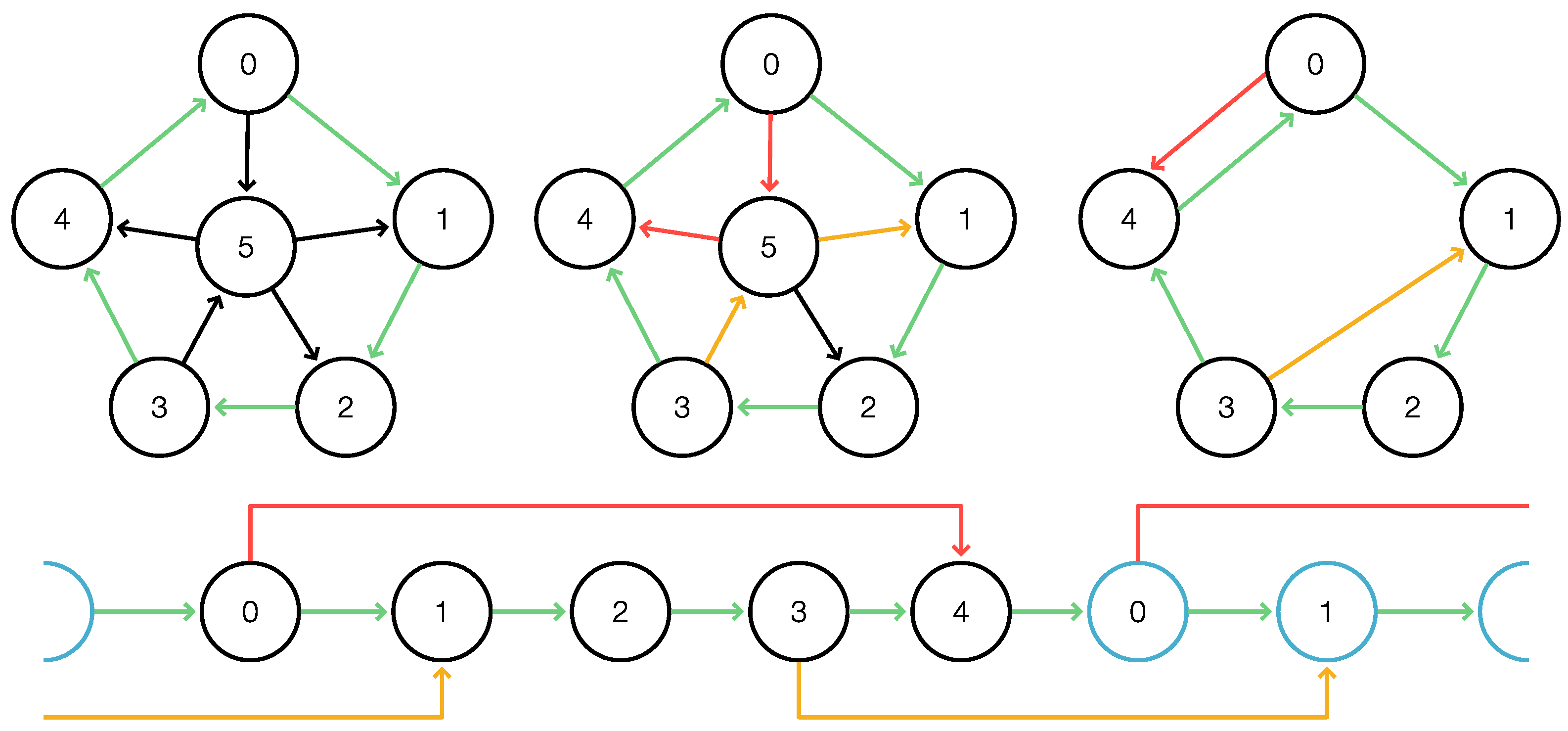
It is well known that the two fundamental traversal orders of trees are obtained as the two natural compositions of the ancestor and the sibling partial orders. Denote by $\rho$ and $\pi$ the order in which vertices are reported in preorder and postorder traversal, respectively. We have:

$$\begin{array}{cc}\hfill \rho \left(x\right)<\rho \left(y\right)& \mathrm{iff}x◃y\mathrm{or}y\prec x\hfill \\ \hfill \pi \left(x\right)<\pi \left(y\right)& \mathrm{iff}x◃y\mathrm{or}x\prec y\hfill \end{array}$$

(1)

It follows immediately that preorder and postorder together determine the ancestor and sibling order:

$$\begin{array}{cc}\hfill x◃y& \mathrm{iff}\rho \left(x\right)<\rho \left(y\right)\mathrm{and}\pi \left(x\right)<\pi \left(y\right)\hfill \\ \hfill x\prec y& \mathrm{iff}\rho \left(x\right)>\rho \left(y\right)\mathrm{and}\pi \left(x\right)<\pi \left(y\right)\hfill \end{array}$$

(2)

Let G be a digraph. For every vertex $r\in V\left(G\right)$, denote by $V\left[r\right]\subseteq V\left(G\right)$ the subset of vertices that are reachable from r, i.e., for which there is a directed path from r to $x\in V\left[r\right]$. These paths can be chosen such that every $x\in V\left[r\right]$ is reachable from r along a unique path, and hence, there is an oriented tree T with $V\left(T\right)=V\left[r\right]$ that is a subgraph of G. An oriented tree T with root r is a search tree on G if there is no directed edge $(x,y)\in E\left(G\right)$ with $x\in V\left(T\right)$ and $y\notin V\left(T\right)$. An ordered tree T is a search tree if and only $V\left(T\right)=V\left[r\right]$ because a vertex $y\in V\left(G\right)\backslash V\left(T\right)$ by definition cannot be reached from anywhere in $V\left(T\right)$, and thus also not from the root, while every $y\in V\left(T\right)$ is by definition reachable from the root r.

Depth-first search (DFS) traverses a digraph G in the following manner: (i) pick a root $r\in V\left(G\right)$; (ii) recursively, at $v\in V\left(G\right)$, proceed to the ◃ smallest, previously-unvisited out-neighbor of v; (iii) if v has no more unvisited out-neighbors, return to is “parent”, i.e., the vertex $par\left(v\right)$ from which v was initially reached [8]. Clearly, DFS generates a rooted tree T with directed edges $\left(par\right(v),v)$, which are known as the DFS-tree.

Lemma 1.

Let T be the ordered subtree generated by DFS on a digraph G, and let $(u,v)\in E\left(G\right)$ with $u\in V\left(T\right)$. Then, $v\in V\left(T\right)$ and either $v\prec u$ (including $(u,v)\in E\left(T\right)$), $u\prec v$, or $v◃u$. In particular, T is a search tree on G.

Proof. 

Consider a DFS reaching u. The search steps up to $par\left(u\right)$ only after exhausting all out-neighbors of u; hence, any edge $(u,v)$ either has been visited before by the DFS process or, otherwise, it is included as an edge as DFS steps down to the subtree of u rooted in v. If v has been accessed before, then v is either an ancestor or descendant of u or u and v are incomparable w.r.t. ≺. In the latter case, there are distinct children x and y of $lca(u,v)$ such that $u\in T\left(x\right)$ and $v\in T\left(y\right)$. In a DFS, $T\left(y\right)$ is traversed before $T\left(x\right)$ if y comes before x in the out-neighbor order of $lca(u,v)$, and thus, $v◃u$.

By the construction of DFS, $x\in V\left(T\right)$ is reachable from the root r along a path in G; hence, $V\left(T\right)\subseteq V\left[r\right]$. Suppose there is $x\in V\left[r\right]\backslash V\left(T\right)$. Along a path p from r to x, let $x^{\prime }$ be the first vertex not reachable from $V\left(T\right)$, i.e., there is an edge $(u,x^{\prime })\in E\left(G\right)$ with $u\in V\left(T\right)$ and $x^{\prime }\notin V\left(T\right)$, contradicting the first assertion of the lemma. □

The DFS process proceeds on $V\left[r\right]$ in such a way that the preorder $\rho$ of the DFS-tree T rooted at r records the order in which the vertices are discovered, while the postorder $\pi$ describes the order in which vertices are completed, i.e., “left”, by ascending back to their parent. To see this, denote by ${\rho }^{\prime }$ and ${\pi }^{\prime }$ the order in which vertices are discovered and completed by DFS started at r. By construction, DFS accesses the out-neighbors of v in ◃ order of the children of v and completes the traversal of a subtree rooted at a child $v^{\prime }$ of v before proceeding to the subtree of another child. Thus, if u and v are incomparable w.r.t. ≺ in T, then ${\rho }^{\prime }\left(u\right)<{\rho }^{\prime }\left(v\right)$ and ${\pi }^{\prime }\left(u\right)<{\pi }^{\prime }\left(v\right)$ if and only if $u◃v$ in the sibling order. It also follows directly from the definition of DFS that we have ${\rho }^{\prime }\left(u\right)<{\rho }^{\prime }\left(v\right)$ if $v\prec u$ and ${\pi }^{\prime }\left(u\right)<{\pi }^{\prime }\left(v\right)$ if $u\prec v$. Hence, ${\rho }^{\prime }$ and ${\pi }^{\prime }$ indeed coincide with the preorder $\rho$ and the postorder $\pi$ for the traversal of DFS tree T. DFS on a graph G is therefore completely described by the oriented DFS tree T, i.e., the sibling and ancestor order on $V\left[r\right]$, and coincides with DFS on T itself.

Hence, the condition that v has been accessed before u can expressed simply as $\rho \left(v\right)<\rho \left(u\right)$. If u and v are comparable on T, their relative order is determined by Equation (2). We therefore obtain the following simple characterization of DFS-trees:

Corollary 1.

A search tree T with postorder ρ on G is a DFS-tree if and only if an edge $(u,v)\in E\left(G\right[V\left(T\right)\left]\right)$ is either (i) a tree edge, (ii) an edge connecting two non-adjacent comparable vertices in T, or (iii) $\rho \left(v\right)<\rho \left(u\right)$ whenever u and v are incomparable w.r.t. ≺ in T.

As a consequence, we have the following classification of edges w.r.t. a DFS-tree. $(u,v)\in E\left(G\right[V\left(T\right)\left]\right)$ is a:

(i)

tree edge iff $(u,v)\in E\left(T\right)$;

(ii)

forward edge iff $(u,v)\notin E\left(T\right)$ and $v\prec u$, i.e., $\pi \left(v\right)<\pi \left(u\right)$ and $\rho \left(v\right)>\rho \left(u\right)$;

(iii)

back edge iff $u⪯v$, i.e., $\pi \left(v\right)\ge \pi \left(u\right)$ and $\rho \left(v\right)\le \rho \left(u\right)$;

(iv)

cross edge iff $u◃v$, i.e., $\pi \left(v\right)<\pi \left(u\right)$ and $\rho \left(v\right)<\rho \left(u\right)$.

2.2. Weak Superbubbloids

Superbubbles [2] are a complex generalization of “bubbles”. Comprising two or more isolated paths connecting a source s to a target t, bubbles are the simplest obstacle in sequence assembly problems [9]. We use here the terminology of [7]:

Definition 1.

Let G be a digraph, and let $(s,t)$ be an ordered pair of distinct vertices. Denote by $U_{st}$ the set of vertices reachable from s without passing through t, and write $U_{ts}^{+}$ for the set of vertices from which t is reachable without passing through s. Then, the subgraph $G\left[U_{st}\right]$ induced by $U_{st}$ is a superbubbloid in G if the following three conditions are satisfied:

(S1)

$t\in U_{st}$, i.e., t is reachable from s (reachability condition).

(S2)

$U_{st}=U_{ts}^{+}$ (matching condition).

(S3)

$G\left[U_{st}\right]$ is acyclic (acyclicity condition).

We call s, t, and $U_{st}\backslash \{s,t\}$ the entrance, exit, and interior of the superbubbloid. We denote the induced subgraph $G\left[U_{st}\right]$ by $⟨s,t⟩$ if it is a superbubbloid with entrance s and exit t.

The reachability and matching conditions can equivalently be expressed in the following form, which usually is more convenient to use:

Lemma 2

([7]).Let G be a digraph, $U\subset V\left(G\right)$, and $s,t\in U$. Then, U equals the set $U_{st}$ of Definition 1 and satisfies (S1) and (S2) if and only if the following conditions (S.i)–(S.iv) are satisfied. Moreover, U forms a superbubbloid with entrance s and exit t if and only if (S.i)–(S.vi) are satisfied:

(S.i)

Every $u\in U$ is reachable from s.

(S.ii)

t is reachable from every $u\in U$.

(S.iii)

If $u\in U$ and $w\notin U$, then every $w\to u$ path contains s.

(S.iv)

If $u\in U$ and $w\notin U$, then every $u\to w$ path contains t.

(S.v)

If $(u,v)$ is an edge in $G\left[U\right]$, then every $v\to u$ path in G contains both t and s.

(S.vi)

G does not contain the edge $(t,s)$.

If only (S.i)–(S.v) holds, the $⟨s,t⟩$ is a weak superbubbloid.

A (weak) superbubble is a (weak) superbubbloid that is minimal in the following sense:

Definition 2.

A (weak) superbubbloid $⟨s,t⟩$ is a (weak) superbubble if there is no $s^{\prime }\in U_{st}\backslash \left\{s\right\}$ such that $⟨s^{\prime },t⟩$ is a (weak) superbubbloid.

Weak superbubbles differ from superbubbles only by (S.vi), which can be checked in constant time for each candidate (weak) superbubble. The effort to recognize superbubbles and weak superbubbles is therefore essentially the same.

The following observation, which summarizes and slightly generalizes our previous analysis [7], forms the basis of the present contribution. As in previous work on the topic [5,6,7], DFS-trees are a key ingredient.

Lemma 3.

Let G be a digraph and $U_{st}$ the vertex set of a weak superbubbloid $⟨s,t⟩$ in G, and suppose r is not an interior vertex or the exit of $⟨s,t⟩$. Then, either $V\left[r\right]\cap U_{st}=\varnothing$ or $U_{st}\subseteq V\left[r\right]$.

Proof. 

(i) Every digraph can be decomposed into strongly-connected components and acyclic components. If $x\in V\left[r\right]$, then every vertex reachable from x is also contained in $V\left[r\right]$. Thus, in particular, every strongly-connected component of G is either contained in $V\left[r\right]$ or disjoint from $V\left[r\right]$. Sung’s theorem ([5] and [7] (Thm.1)) ensures that every superbubbloid is either contained in a strongly- connected component C or an acyclic component A of G. Now, suppose $V\left[r\right]\cap U_{st}\ne \varnothing$, and let $x\in U_{st}$ be the first vertex of the DFS in $⟨s,t⟩$. By definition (of weak superbubbloids) $x=s$, since no other vertex in $U_{st}$ is reachable from outside $U_{st}$, and the DFS assumption does not start at an interior vertex or the exit of $⟨s,t⟩$. The reachability axiom (S.ii) ensures that every $u\in U_{st}$ is reached by the DFS whenever $s\in V\left(G\right)$, i.e., $U_{st}\in V\left[r\right]$. □

Lemma 3 is a variant of the key theorem of [5].

Corollary 2.

Let $G=(V,E)$ be a digraph and $U_{st}$ the vertex set of a weak superbubbloid $⟨s,t⟩$ in G. Let $r_1,r_2,\cdots ,r_k\in V$ be such that none of the $r_i$ are an interior or an exit vertex of $⟨s,t⟩$. Set $W_j:={\bigcup }_{i=1}^{j}V\left[r_i\right]$ and $V^{\prime }\left[r_j\right]=V\left[r_j\right]\backslash W_{j-1}$. Then, either $U_{st}\cap V^{\prime }\left[r_j\right]=\varnothing$ or $U_{st}\subseteq V^{\prime }\left[r_j\right]$.

Proof. 

By Lemma 3, $U_{st}$ is either contained in the intersection of two or more reachable sets $V\left[r_i\right]$ or is disjoint from it. As an immediate consequence, it is also either contained in the difference of two reachable sets or disjoint from it. □

Lemma 4.

Let G be a digraph; let $U_{st}$ be the vertex set of a weak superbubbloid $⟨s,t⟩$ in G; let T be a DFS-tree on G with root $r\notin U_{st}\backslash \left\{s\right\}$; and let π be the postorder w.r.t. T. Then:

(i) 

The induced subgraph $G\left[U_{st}\right]$ contains no back edges w.r.t. T, except possibly $(t,s)$.

(ii) 

If $U_{st}\subseteq V\left(T\right)$, then $\left\{\pi \left(u\right)\right|u\in U_{st}\}=[\pi \left(t\right),\pi \left(s\right)]$ is an interval w.r.t. to π.

Proof. 

(i) The statement is trivial if $⟨s,t⟩$ is not contained in T. If $⟨s,t⟩$ resides in an acyclic part A of G, there are no back edges because A cannot contain back edges by acyclicity. If $⟨s,t⟩$ is contained in a strongly-connected component C, the proof of Lemma 9 of [7] also implies Assertion (i) because the DFS-tree T, in particular, contains a DFS-tree of C as a subtree and back edges in G can only be located within a strongly-connected component.

(ii) Since the DFS generating T enters $⟨s,t⟩$ through s and leaves it through t, the preorder $\rho$ satisfies $\rho \left(s\right)<\rho \left(t\right)$. Since t is reachable from every $u\in U_{st}$, we conclude that any DFS reaches t before completing any $u\in U_{st}$; hence, t precedes any other $u\in U_{st}$ in postorder, i.e., $\pi \left(u\right)>\pi \left(t\right)$. Since $u\in U_{st}$ is not reachable without passing through s, every other vertex in $u\in U_{st}$ precedes s in postorder, i.e., $\pi \left(s\right)>\pi \left(u\right)$. Now, suppose there is some $w\notin U_{st}$ with $\pi \left(s\right)>\pi \left(w\right)>\pi \left(t\right)$. Then, w must be reachable from s along a directed path that does not pass through t, a contradiction to the definition of weak superbubbloids. Hence, the vertices of a superbubbloid form an interval in postorder of the DFS-tree T. □

Statement (ii) rephrases the key result of [6], although we do not need to assume that G is an acyclic digraph. Conceptually, Lemma 4 suggests that it might not be necessary to first identify the strongly-connected components of G [5] or the construct acyclic auxiliary digraphs [6] in order to find all weak superbubbles. Lemma 2 then ensures that a single DFS-forest is sufficient.

2.3. Superbubble Detection

We next show how to retrieve all weak superbubbles of a digraph G that are located within the induced subgraph $G\left[V\right[r\left]\right]$ of G. To this end, we use a slightly modified version of the algorithm DAGsuperbubble described in [7]. It was originally designed to operate on acyclic auxiliary graphs with a single source. Thus, it could be assumed that a DFS-tree rooted on this source reached all vertices. Here, we intend to apply it to the unmodified input graph, which is neither acyclic, nor guaranteed to have a single source. It, therefore, needs to be modified to deal appropriately with back edges within the DFS-tree and the existence of vertices outside the DFS-tree. To this end, vertices in $V\left[r\right]$ that cannot be contained in a superbubble have to be identified. By Lemma 4, there are two possible obstructions for a vertex u: (i) u has an edge that is a back edge in the DFS-tree; (ii) u is incident to an edge $(x,u)$ or $(u,x)$ where $x\notin V\left[r\right]$.

The basic idea of DAGsuperbubble is to identify minimal intervals in reverse postorder $\overline{\pi }:=\left|V\left[r\right]\right|-\pi \left(v\right)-1$ of the DFS-tree T that satisfy conditions equivalent to membership in a superbubbloid. These conditions are expressed in terms of a pair of helper functions with the help of reverse postorder $\overline{\pi }\left(v\right)$ on T. As in [7], $\mathbf{OutParent}\left(v\right)$ denotes the first vertex (w.r.t. reverse postorder $\overline{\pi }$) in T from which v can be reached. Similarly, $\mathbf{OutChild}\left(v\right)$ is the last child vertex reachable from v.

$$\begin{array}{cc}\hfill \mathbf{OutParent}\left(v\right)& :=\left\{\begin{array}{cc}-1\hfill & \mathrm{if}\mathrm{no}(u,v)\in E\left(G\right)\mathrm{exists}\hfill \\ -1\hfill & \mathrm{if}(u,v)\in E\left(G\right)\wedge u\notin V\left[r\right]\hfill \\ -1\hfill & \mathrm{if}\mathrm{a}\mathrm{back}\mathrm{edge}(u,v)\in E\left(G\right)\hfill \\ min\left(\left\{\overline{\pi }\left(u\right)\right|(u,v)\in E\left(G\right)\}\right)\hfill & \mathrm{otherwise}\hfill \end{array}\right.\hfill \\ \hfill \mathbf{OutChild}\left(v\right)& :=\left\{\begin{array}{cc}\infty \hfill & \mathrm{if}\mathrm{no}(v,u)\in E\left(G\right)\mathrm{exists}\hfill \\ \infty \hfill & \mathrm{if}(v,u)\in E\left(G\right)\wedge u\notin V\left[r\right]\hfill \\ \infty \hfill & \mathrm{if}\mathrm{there}\mathrm{is}\mathrm{a}\mathrm{back}\mathrm{edge}(v,u)\in E\left(G\right)\hfill \\ max\left(\left\{\overline{\pi }\left(u\right)\right|(v,u)\in E\left(G\right)\}\right)\hfill & \mathrm{otherwise}\hfill \end{array}\right.\hfill \end{array}$$

(3)

These functions are extended to intervals on $\overline{\pi }$ as follows:

$$\begin{array}{cc}\hfill \mathbf{OutParent}\left(\right[i,j\left]\right)& :=min\{\mathbf{OutParent}\left(v\right)\mid v\in V\left[r\right]\wedge i\le \overline{\pi }\left(v\right)\le j\}\hfill \\ \hfill \mathbf{OutChild}\left(\right[i,j\left]\right)& :=max\{\mathbf{OutChild}\left(v\right)\mid v\in V\left[r\right]\wedge i\le \overline{\pi }\left(v\right)\le j\}\hfill \end{array}$$

(4)

In [7], we derived a characterization of weak superbubbloids in terms of $\mathbf{OutParent}\left(\right[i,j\left]\right)$ and $\mathbf{OutChild}\left(\right[i,j\left]\right)$ for the case of acyclic digraphs. Here, we generalize this condition to general graph using the modified definition of $\mathbf{OutParent}\left(v\right)$ and $\mathbf{OutChild}\left(v\right)$. The difference is that the situation that back edges and edges connecting to the outside of the DFS-tree are considered. In either case, the corresponding vertices are marked by $-1$ or ∞, respectively, to indicate that they cannot be part of superbubbloids.

Theorem 1.

Let G be a digraph; let T be a DFS-tree on G with a root r that is not an interior vertex or exit of a weak superbubbloid; and denote by $\overline{\pi }$ the reverse postorder on T. Then, $⟨s,t⟩$ is a weak superbubbloid in G whose vertex set $U_{st}$ satisfies $U_{st}\cap V\left[r\right]\ne \varnothing$ if and only if the following conditions are satisfied:

(F1)

$\mathbf{OutParent}\left([\overline{\pi }\left(s\right)+1,\overline{\pi }\left(t\right)]\right)=\overline{\pi }\left(s\right)$ (predecessor property)

(F2)

$\mathbf{OutChild}\left([\overline{\pi }\left(s\right),\overline{\pi }\left(t\right)-1]\right)=\overline{\pi }\left(t\right)$ (successor property)

Proof. 

It was shown in [7] (theorem 2) that the statement is true for acyclic digraphs. We first note that by Lemma 3, every weak superbubbloid intersecting $V\left[r\right]$ is contained in $V\left[r\right]$, i.e., in $V\left(T\right)$. For the purpose of the proof, consider the auxiliary graph $\widehat{G}\left[V\left(T\right)\right]$ with edge set $E\left(\widehat{G}\left[V\left(T\right)\right]\right)=E\left(G\left[V\left(T\right)\right]\right)\backslash \{e\mid e\mathrm{is}\mathrm{a}\mathrm{back}\mathrm{edge}\mathrm{w}.\mathrm{r}.\mathrm{t}.\mathrm{T}\}$. By construction, $\widehat{G}\left[V\left(T\right)\right]$ is acyclic, and every vertex is in T. Thus, every superbubbloid $⟨s,t⟩$ (with vertex set $U_{st}$) in $\widehat{G}\left[V\left(T\right)\right]$ is characterized by Conditions (F1) and (F2). It is, furthermore, a weak superbubbloid in G if and only if the following conditions hold:

(i)

For every $u\in U_{st}\backslash \left\{s\right\}$, there is no edge $(x,u)\in E\left(G\right)$ such that $x\notin U_{st}$;

(ii)

For every $v\in U_{st}\backslash \left\{t\right\}$, there is no edge $(v,x)\in E\left(G\right)$ such that $x\notin U_{st}$; and

(iii)

$G\left[U_{st}\right]$ without the edge $(t,s)\in E\left(G\right)$ acyclic.

Only edges not contained in $\widehat{G}\left[V\left(T\right)\right]$ need to be considered for Conditions (i) and (ii), because no such edges exist within $\widehat{G}\left[V\left(T\right)\right]$ due to the assumption that $⟨s,t⟩$ is a weak superbubbloid in $\widehat{G}\left[V\left(T\right)\right]$. For (iii), only the back edges are of interest. By definition, a back edge creates a cycle in $\widehat{G}\left[V\left(T\right)\right]$. A back edge $(v^{\prime },u^{\prime })$ with $u^{\prime }\in U_{st}$ would violate (iii) when $v^{\prime }\in U_{st}$ or (i) if $v^{\prime }\notin U_{st}$. Analogously, if $v^{\prime }\in U_{st}$ and $u^{\prime }\notin U_{st}$, then (ii) is violated. Thus, a weak superbubbloid cannot contain the head or tail of a back edge. Only for Condition (i), we also need to consider the case that $x\notin V\left(T\right)$.

(F1) can be satisfied only if $\mathbf{OutParent}\left(u\right)>-1$ for every $u\in U_{st}\backslash \left\{s\right\}$. Analogously, (F2) can only be true if $\mathbf{OutChild}\left(u\right)<\infty$ for all $u\in U_{st}\backslash \left\{t\right\}$. Hence, it suffices to rule out false positive weak superbubbloids in G by ensuring that every vertex u that violates one of the three conditions also violates (F1) or (F2). This is achieved by setting $\mathbf{OutParent}\left(u\right)=-1$ for a vertex u if there is an edge $(x,u)$ such that $x\notin V\left(T\right)$ or $(x,u)$ is a back edge; analogously, we set $\mathbf{OutChild}\left(v\right)=\infty$ for all v with an incident edge $(v,x)$ such that $x\notin V\left(T\right)$ or $(v,x)$ is a back edge. Equation (3) implements exactly these conditions. Thus, only weak superbubbloids fulfill (F1) and (F2).

Conversely, it suffices to note that by Lemma 4(ii), every weak superbubbloid forms a contiguous interval w.r.t. the postorder $\pi$ of T and, thus, also w.r.t. the reverse postorder $\overline{\pi }$ of T. □

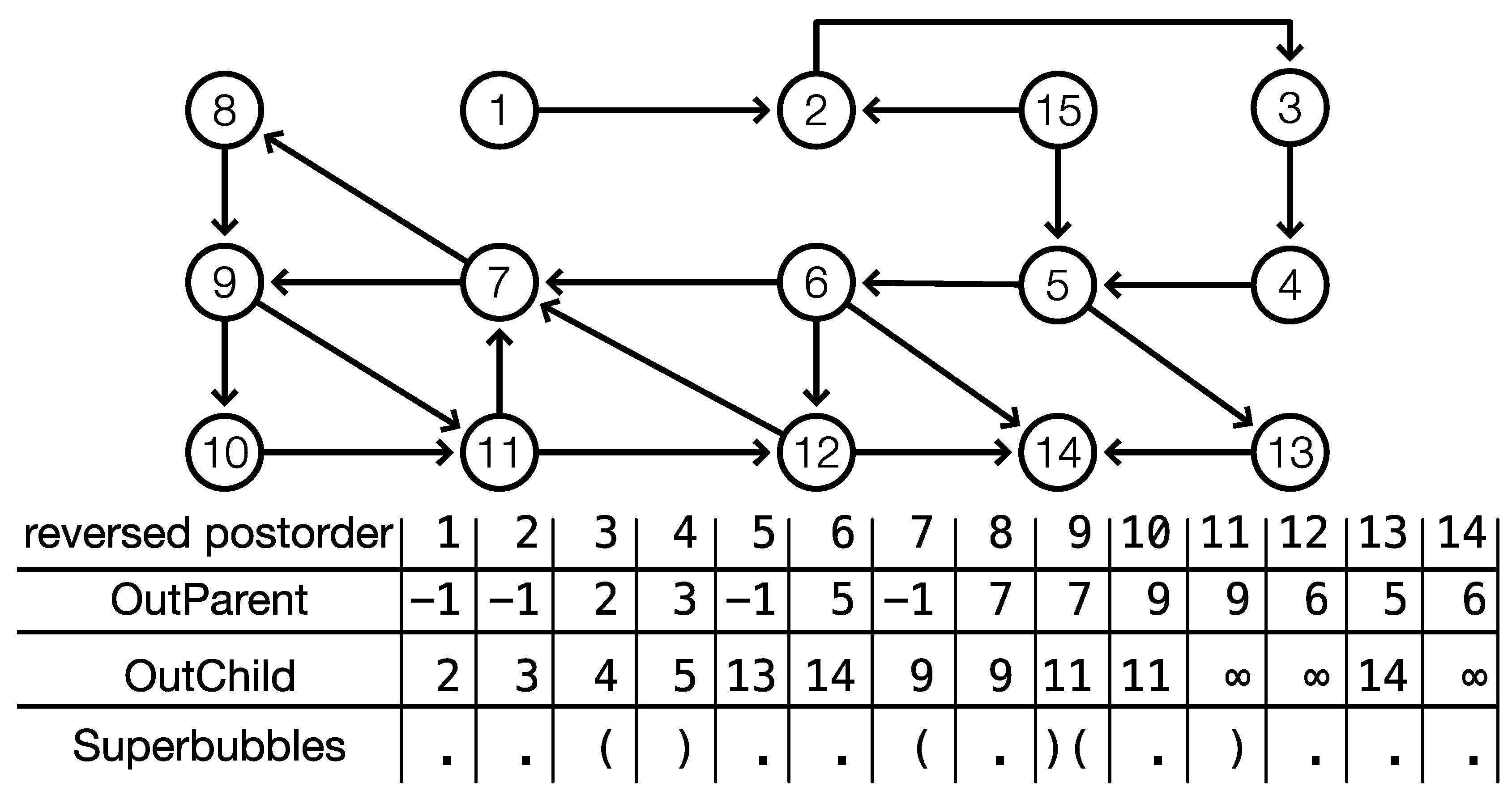
We denote by Superbubble the algorithm DAGsuperbubble with the modified functions $\mathbf{OutParent}(.)$ and $\mathbf{OutChild}(.)$ as described above. By construction, Superbubble identifies minimal intervals of $\overline{\pi }$ that satisfy (F1) and (F2); see Figure 1 for an illustration and [7] for full details. Since the modification of $\mathbf{OutParent}(.)$ and $\mathbf{OutChild}(.)$ only amounts to setting additional entries to $-1$ or ∞, respectively, the performance remains unaffected. According to Theorem 1, the minimal intervals satisfying (F1) and (F2) are exactly the minimal weak superbubbloids and, thus, by definition, the weak superbubbles. Therefore, we have:

Figure 1. Illustration of the algorithm Superbubble on a digraph G with cycles. The top panel shows the input digraph. The DFS-tree T is rooted at one and covers $V\left[r\right]=V\left(G\right)\backslash \left\{15\right\}$. The table below gives the values of $\mathbf{OutParent}$ and $\mathbf{OutChild}$ as a function of the reverse postorder $\overline{\pi }$ of T. In the final line, matching pairs of parentheses indicate entrances and exits of the weak superbubbles in $V\left[r\right]$. This corresponds to the intervals that fulfill (F1) and (F2).

Corollary 3.

Let G be a digraph, and let T be a DFS-tree on G with a root r that is not an interior vertex or exit of a weak superbubble. Then,Superbubblecorrectly identifies exactly the weak superbubbles $⟨s,t⟩$ in G whose vertex set satisfies $U_{st}\cap V\left[r\right]\ne \varnothing$.

It is straightforward to extend this result to a DFS-forest that covers $V\left(G\right)$ entirely: This forest is constructed by first constructing $T_1$ with root $r_1$ covering $V\left[r_1\right]$. Then, $T_2$ is constructed from a root $r_2$ searching on $V\left(G\right)\backslash V\left[r_1\right]$, and so on; see Lemma 2. This amounts to constructing an auxiliary graph $G^{\prime }$ from G by adding an artificial root $r_0$ and out-edges $(r_0,r_1)$, $(r_0,r_2)$,..., $(r_0,r_k)$, and defining the sibling order of the roots as $r_1◃r_2◃\cdots ◃r_k$. The DFS-forest $F(r_1,\cdots ,r_k)$ with given roots $r_1$, $r_2$,..., $r_k$ on G is then equivalent to the DFS-tree $T^{\prime }$ rooted at $r_0$ on $G^{\prime }$ if we define the reverse postorder of $T^{\prime }$ such that $\overline{\pi }\left(r_0\right)=0$. We note, furthermore, that sibling order, i.e., the order in which the roots are used to seed DFS, is arbitrary.

Corollary 4.

Let G be a digraph, and let F be a DFS-forest on G comprising DFS-trees $T_i$ with roots $r_i$, $1\le i\le k$, none of which is an interior vertex or exit of a weak superbubble. Let $\overline{\pi }$ be the reverse postorder on F, obtained by concatenating the reverse postorders on the constituent DFS-trees. Then,Superbubblecorrectly identifies exactly the weak superbubbles $⟨s,t⟩$ in G. Furthermore, given the roots $r_i$,Superbubblehas a running time of $O\left(\right|E|+|V\left|\right)$.

Proof. 

Correctness follows immediately from Corollary 3, the construction of $T^{\prime }$ on the auxiliary digraph $G^{\prime }$, and Lemma 2. During the DFS, each out-edge is considered exactly once, and each vertex is traversed twice. The number k of required roots is limited by $\left|V\right|$. For each vertex v, checking whether $\mathbf{OutParent}\left(v\right)=-1$ or $\mathbf{OutChild}\left(v\right)=\infty$ requires checking all neighbors only; hence, the total effort is no more than $O\left(\right|E|+|V\left|\right)$. The linear time complexity of DAGsuperbubble, finally, is proven in [7]. □

It is important to note the correctness of Superbubble, Corollary 3, crucially depends on the correct choice of the root r of the DFS-tree. The remaining problem thus is to find a suitable sequence of roots $r_1$, $r_2$,..., $r_k$.

Definition 3.

A vertex $r\in V$ is a legitimate root if for every weak superbubble $⟨s,t⟩$ in G with vertex set $U_{st}$, we have either $U_{st}\subseteq V\left[r\right]$ and $t\prec s$ (in the ancestor order of a search tree with root r), or $U_{st}\cap V\left[r\right]=\varnothing$.

We can summarize the discussion in the following form:

Corollary 5.

The algorithmSuperbubbledetects all weak superbubbles in G if and only if there is a set $\{r_1,r_2,\cdots ,r_k\}$ of legitimate roots such that the DFS-forest $F(r_1,r_2,\cdots ,r_k)$ covers $V\left(G\right)$.

Corollary 6.

A vertex $r\in V$ is a legitimate root if and only if r is neither an interior nor an exit of a weak superbubble.

Proof. 

By Corollary 4, a root is legitimate if it is not the exit or an interior vertex of a weak superbubble. Conversely, if r is an interior vertex or the exit of $⟨s,t⟩$, then a DFS-tree rooted in r reaches the entrance s either not at all or there is not search tree with root r such that $t\prec s$, since by definition of a weak superbubble, the exit t is found before s along every path from r to s. □

Lemma 5.

Let G be a digraph and $v\in V\left(G\right)$ a source, i.e., a vertex with in-degree zero. Then, v is a legitimate root.

Proof. 

Since v is not reachable from any other vertex, it is only reachable by DFS if the traversal starts in v. By the same argument, v is neither an interior vertex, nor the exit of a weak superbubble and, thus, is a legitimate root. □

Unfortunately, there is no guarantee that a digraph G has source vertices, and even if they exist, not every vertex of G is necessarily reachable from them. The task is, therefore, to identify legitimate roots located within strongly-connected components.

2.4. Cycles, $\stackrel{C}{⇝}$-Covers, and $\stackrel{C}{⇝}$-Cuts

Definition 4.

Let G be a digraph. A set $C=\{c_1,\cdots ,c_k\}\subseteq V\left(G\right)$ is a cycle in G if $k=\left|C\right|$ and $E\left(C\right):=\{(c_1,c_2),\cdots ,(c_{k-1},c_k),(c_k,c_1)\}\subset E\left(G\right)$. A pair of vertices $c_i,c_j\in C$ determines a cycle interval:

$$c_i,c_j:=\left\{\begin{array}{cc}{c}_{i+1},\cdots ,c_{j-1}\hfill & \mathrm{if}i<j\hfill \\ c_{i+1},\cdots ,c_k\cup c_1,\cdots ,c_{j-1}\hfill & otherwise\hfill \end{array}\right.$$

By definition, the vertices $c_i$ are pairwise distinct and indexed consecutively along C. Importantly, cycle intervals contain only the interior of the unique path in C connecting the defining endpoints $c_i$ and $c_j$. Thus, $c_1,c_2=\varnothing$ if $(c_1,c_2)\in E\left(C\right)$ and $v,v=C\backslash \left\{v\right\}$ for all $v\in C$. The C-distance of two vertices $c_i$ and $c_j$ along a cycle C is the length of the directed path, i.e., the number of edges, from $c_i$ to $c_j$. More explicitly,

$$d_C(c_i,c_j):=\left\{\begin{array}{cc}j-i\hfill & \mathrm{if}i<j\hfill \\ j-i+k\hfill & \mathrm{if}i\ge j\hfill \end{array}\right.=\left|c_i,c_j\right|+1$$

(5)

since the number of inner vertices is one less than the number of edges. In particular, $d_C(v,v)=\left|C\right|$ for all $v\in C$. The C-distance $d_C$ is not symmetric. Instead, we have $d_C(u,v)+d_C(v,u)=\left|C\right|$ for all two vertices $u\ne v\in C$. Another useful consequence of the definition of $d_C$ is:

$$d_C(v,w)<d_C(v,u)\Rightarrow d_C(w,u)=d_C(v,u)-d_C(v,w)$$

(6)

The following implication will be useful later on:

Corollary 7.

Let G be a digraph; let C a cycle in G; and let $c_1,c_2,c_3\in C$. Then, $d_C(c_1,c_2)\le d_C(c_1,c_3)$ if and only if $c_1\in c_3,c_2\cup \left\{c_3\right\}$.

Proof. 

If $c_1$, $c_2$, and $c_3$ are pairwise distinct, the l.h.s. is true if the path from $c_1$ to $c_2$ is a subpath of the path from $c_1$ to $c_3$, i.e., $c_1\notin c_2,c_3$ and, thus, $c_1\in c_3,c_2\cup \left\{c_3\right\}$. The converse is obvious. The statement is trivial for $c_1=c_3$. If $c_2=c_3$, the l.h.s. is always true, while on the r.h.s., we have $c_2,c_2\cup \left\{c_2\right\}=C\ni c_1$. For $c_1=c_2$, both the l.h.s. and the r.h.s. are satisfied only if $c_2=c_3$. □

In the following, it will be useful to know whether two vertices on a cycle are also reachable via a directed path that is disjoint from C. We formalize this idea as a binary relation on C.

Definition 5.

Let G be a digraph and C a cycle in G and $s,t\in V$. Then, t isC-reachable from s, in symbols $s\stackrel{C}{⇝}t$, if there is a path $p=\{s=v_0,\cdots v_h=t\}$ such that $h\ge 1$ and $v_i\notin C$ for $0<i<h$.

We have used the letters s and t here since C-reachability will be used to identify potential candidates for entrance and exit of superbubbles. C-reachability is defined not only for vertices in the “reference cycle” C. It satisfies a restricted transitivity property: If $v\in V\left(G\right)\backslash C$, $s\stackrel{C}{⇝}v$, and $v\stackrel{C}{⇝}t$, then $s\stackrel{C}{⇝}t$. Another interesting observation is that $s\stackrel{C}{⇝}s$ implies that there is a directed cycle $C^{\prime }$ such that $C\cap C^{\prime }=\left\{s\right\}$. As an immediate consequence of Definition 5, we obtain:

Lemma 6.

Let G be a digraph, C a cycle in G, $c_1,c_2\in C$ such that $c_1\stackrel{C}{⇝}{c}_2$, and $d_C(c_1,c_2)>1$. Then, $c_1$ and $c_2$ are connected by (at least) two edge-disjoint directed paths. In particular, $\{(v_i,v_{i+1})\mid 0\le i<h\}\cap E\left(C\right)=\varnothing$.

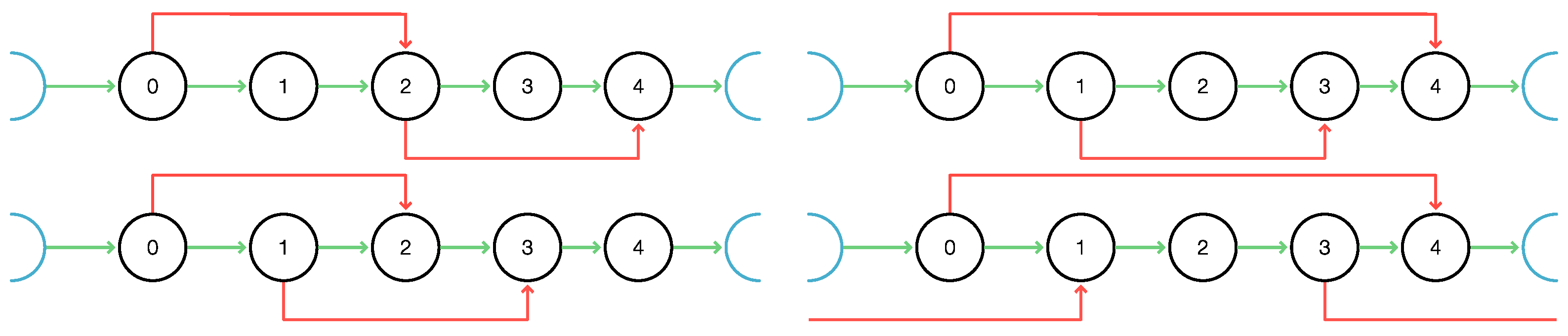
Definition 6.

Let C be a cycle in the digraph G and $u,v\in C$. Then, $u,v$ is$\stackrel{C}{⇝}$-covered if $u\stackrel{C}{⇝}v$.

As an immediate consequence of the definition, $v\stackrel{C}{⇝}v$ implies that $C\backslash \left\{v\right\}$ is covered, while nothing is covered if $(u,v)\in E\left(C\right)$.

Consider two C-intervals $u,v$ and $x,y$ on the same cycle C of the digraph G. We say that $u,v$ is included in $x,y$ if $u,v⊊x,y$, $u,v$ and $x,y$ are disjoint if $u,v\cap x,y=\varnothing$, and $x,y$ extends $u,v$ if $d_C(x,v)<d_C(u,v)$ and $d_C(x,v)<d_C(x,y)$. In particular, if $x,y$ extends $u,v$, then $x\in u,v$, since the interval boundaries themselves are not considered part of the C-intervals. For each pair of distinct C-intervals, thus exactly one of the following four statements is true: (a) the C-interval are disjoint; (b) one C-interval is contained in (i.e., a proper subset of) the other one; (c) one C-interval, say $x,y$, extends the other one, but not vice versa, i.e., $x\in u,v$ and $y\notin u,v$; (d) both C-intervals extend each other, i.e., $x,y\in u,v$. Figure 2 illustrates the four cases. Note that in Case (c), the interval boundaries are arranged in the order $u-x-v-y-u$ along the cycle, while in Case (d), the arrangement is $u-y-x-v-u$ along C.

Figure 2. Relationships of distinct C-intervals. The four possibilities for the relative location of two distinct C-intervals are shown on a linear layout of a cycle C with five vertices ($0,1,2,3,4$). Left top: the C-intervals $0,2$ and $2,4$ are disjoint. Right top: $0,4$ includes $1,3$. Left bottom: $1,3$ extends $0,2$, but not vice versa. Right bottom: $0,4$ and $3,1$ extend each other. Together, the two C-intervals cover C.

In the following, we will use the notation:

$$\begin{array}{cc}\hfill \mathfrak{Q}\left(C\right)& :=\{u,v\mid u\stackrel{C}{⇝}v,u,v\in C\}\hfill \\ \hfill Q\left(C\right)& :=\bigcup _{B\in \mathfrak{Q}\left(C\right)}B=\{w\mid \exists B\in \mathfrak{Q}\left(C\right):w\in B\}\hfill \end{array}$$

(7)

for the set of all $\stackrel{C}{⇝}$-covered intervals and the set of all $\stackrel{C}{⇝}$-covered vertices of C, respectively. Note that $\varnothing \in \mathfrak{Q}\left(C\right)$ since $u\stackrel{C}{⇝}v$ holds for $(u,v)\in E\left(C\right)$. By the same argument, there is at least one interval $u,v\in \mathfrak{Q}\left(C\right)$ for each $u\in C$, albeit some or even all of these may be empty.

Definition 7.

A subset $\mathfrak{B}\subseteq \mathfrak{Q}\left(C\right)$ is a$\stackrel{C}{⇝}$-cover of C if ${\bigcup }_{B\in \mathfrak{B}}B=Q\left(C\right)$, and $\mathfrak{B}$ is a total $\stackrel{C}{⇝}$-cover of C if ${\bigcup }_{B\in \mathfrak{B}}B=C$. We say that C is totally $\stackrel{C}{⇝}$-covered if C has a total $\stackrel{C}{⇝}$-cover.

Note that C is totally $\stackrel{C}{⇝}$-covered if and only if $Q\left(C\right)=C$.

Definition 8.

A vertex in $v\in K\left(C\right):=C\backslash Q\left(C\right)$ is a$\stackrel{C}{⇝}$-cut vertex.

Obviously, C is either totally $\stackrel{C}{⇝}$-covered or it has a non-empty set $K\left(C\right)$ of $\stackrel{C}{⇝}$-cut vertices.

Definition 9.

Let C be a cycle in the digraph G. A$\stackrel{C}{⇝}$-cover $\mathfrak{B}$ of C is clean if $B\in \mathfrak{B}$ and $B^{\prime }⊊B$ implies $B^{\prime }\notin \mathfrak{B}$.

In other words, in a clean $\stackrel{C}{⇝}$-cover, no $\stackrel{C}{⇝}$-covered interval is contained within another one.

Corollary 8.

Let C be a cycle in the digraph G, and let $\mathfrak{B}$ be a clean $\stackrel{C}{⇝}$-cover. Then, either $\mathfrak{B}=\{\varnothing \}$ or, for every $C(u,v)\in \mathfrak{B}$, $d_C(u,v)>1$.

Proof. 

Recall that $C(u,v)=\varnothing$ if and only if $d_C(u,v)=1$. Thus, $\mathfrak{Q}\left(C\right)=\{\varnothing \}$ if and only if there is no $u,v\in \mathfrak{B}$ with $d_C(u,v)>1$. Since the empty set is a subset of every other set, $d_C(u,v)>1$ for every $u,v\in \mathfrak{B}$ unless $\mathfrak{B}=\mathfrak{Q}\left(C\right)=\{\varnothing \}$. □

Lemma 7.

Let C be a cycle in the digraph G. Then, $\mathfrak{Q}\left(C\right)$ contains a clean $\stackrel{C}{⇝}$-cover $\mathfrak{B}$.

Proof. 

Let $\mathfrak{B}\subseteq \mathfrak{Q}\left(C\right)$ be a set of $\stackrel{C}{⇝}$-covered intervals that together $\stackrel{C}{⇝}$-cover $Q\left(C\right)$. Suppose $\mathfrak{B}$ is not clean. Then, there are two intervals $p,q\in \mathfrak{B}$ and $u,v\in \mathfrak{B}$ such that $p,q⊊u,v$. Then, ${\mathfrak{B}}^{\prime }=\mathfrak{B}\backslash \left\{p,q\right\}$ still $\stackrel{C}{⇝}$-cover $Q\left(C\right)$. The removal of such redundant intervals can be repeated until no further removable interval can be found. By Definition 9, the remaining $\stackrel{C}{⇝}$-cover is clean. □

Definition 10.

Let C be a cycle in a digraph G. Then:

$$\mathfrak{L}\left(C\right)=\left\{u,v\in \mathfrak{Q}\left(C\right)\mid forall{v}^{\prime }\in Candu,v^{\prime }\in \mathfrak{Q}\left(C\right),d_C(u,v^{\prime })\le d_C(u,v)\right\}$$

By definition, $\mathfrak{L}\left(C\right)$ consists of all $\stackrel{C}{⇝}$-covered intervals for which there is no larger $\stackrel{C}{⇝}$-covered interval with the same starting point. Since every $p,q\in \mathfrak{Q}\left(C\right)\backslash \mathfrak{L}\left(C\right)$ is contained in a interval with the same starting point, $\mathfrak{L}\left(C\right)$ is a $\stackrel{C}{⇝}$-cover of C. Thus, Lemma 7 implies:

Corollary 9.

Let C be a cycle in a digraph G. Then, there is clean cover $\mathfrak{B}\subseteq \mathfrak{L}\left(C\right)$.

Lemma 8.

Let C be a cycle in the digraph G. A clean $\stackrel{C}{⇝}$-cover $\mathfrak{B}$ of C is total if and only if $\mathfrak{B}\ne \varnothing$ and every $B\in \mathfrak{B}$ is extended by at least one $B^{\prime }\in \mathfrak{B}$.

Proof. 

If $\mathfrak{B}=\varnothing$, then $Q\left(C\right)=\varnothing$, and thus, $\mathfrak{B}$ is not total. In the following, we assume $\mathfrak{B}\ne \varnothing$ is a clean $\stackrel{C}{⇝}$-cover. Suppose, for contradiction, that $u,v\in \mathfrak{B}$ is not extended by any $B\in \mathfrak{B}$. Then, any interval $B^{\prime }\in \mathfrak{B}$ $\stackrel{C}{⇝}$-covering v would have to contain $u,v$, contradicting the assumption that $\mathfrak{B}$ is clean. Thus, v is a $\stackrel{C}{⇝}$-cut vertex, and hence, $\mathfrak{B}$ is not total. If $\mathfrak{B}$, therefore it is non-empty, and every $B\in \mathfrak{B}$ is extended by some $B^{\prime }\in \mathfrak{B}$.

Conversely, suppose c is a $\stackrel{C}{⇝}$-cut vertex of C. If $u,c\in \mathfrak{B}$ for some u, then the first part of the proof implies that $u,c$ is not extended by any $B^{\prime }\in \mathfrak{B}$. If $\mathfrak{B}$ contains no interval $u,c$, then consider the vertex v such that $u,v\in \mathfrak{B}$ for which $d_C(v,c)$ is minimal. Since c is a $\stackrel{C}{⇝}$-cut vertex, there is no extension of $u,v$, since any such extension $B^{\prime }$ would either contradict the minimality of $d_C(v,c)$ or $\stackrel{C}{⇝}$-cover c, thereby contradicting the assumption that c is a $\stackrel{C}{⇝}$-cut vertex. Thus, v is again a $\stackrel{C}{⇝}$-cut vertex. As shown in the first part of the proof, $u,v$; therefore, it is not extended by any $B\in \mathfrak{B}$. We conclude that unless $\mathfrak{B}$ is a total $\stackrel{C}{⇝}$-cover or $\mathfrak{B}=\varnothing$, there is an interval $B\in \mathfrak{B}$ without an extension. □

Figure 3 shows an example of a cycle with a total $\stackrel{C}{⇝}$-cover and a cycle with a $\stackrel{C}{⇝}$-cut, respectively. Since the largest $\stackrel{C}{⇝}$-interval in C is $v,v=C\backslash \left\{v\right\}$ for some v, every total $\stackrel{C}{⇝}$-cover comprises at least two $\stackrel{C}{⇝}$-covered intervals.

Figure 3. $\stackrel{C}{⇝}$-covers. (a) The green cycle C in the top panel has five $\stackrel{C}{⇝}$-paths indicated in red. In the middle panel, C is laid out linearly to emphasize the $\stackrel{C}{⇝}$-covered intervals. Below, the clean $\stackrel{C}{⇝}$-cover obtained by removing all $\stackrel{C}{⇝}$-intervals that are contained in longer ones. Note that every $\stackrel{C}{⇝}$-interval is extended by another one; hence, the $\stackrel{C}{⇝}$-cover is total. (b) Again, the top panel highlights C in green and the $\stackrel{C}{⇝}$-paths in red. The linear layout below highlights that Vertex 1 is not $\stackrel{C}{⇝}$-covered. Thus, it is a $\stackrel{C}{⇝}$-cut vertex.

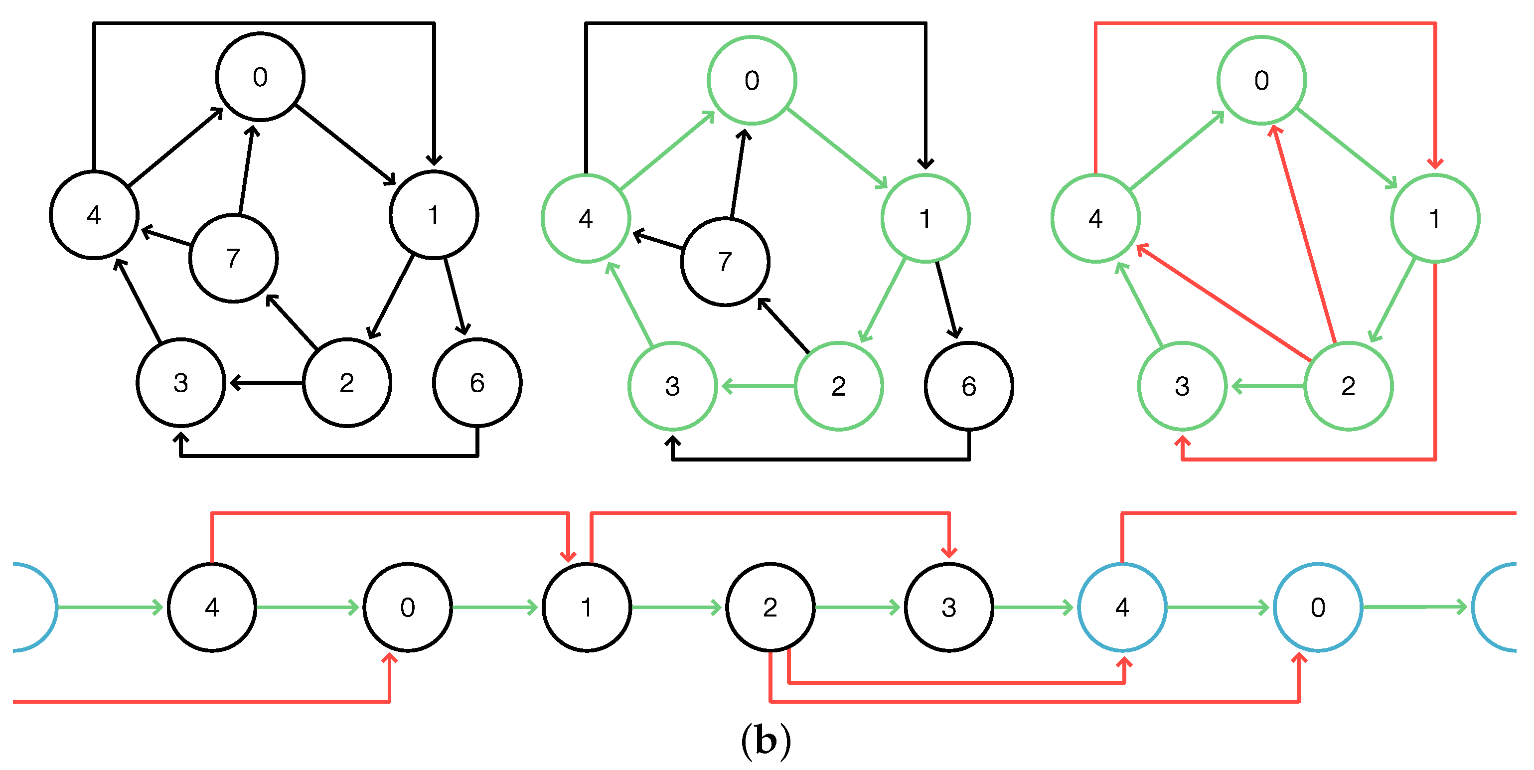
The following lemma provides us with a convenient way to obtain a total $\stackrel{C}{⇝}$-cover.

Lemma 9.

Let C be a cycle in G, $v\notin C$, and $c_1,c_2,c_3,c_4\in C$ with $d_C(c_1,c_3)\le d_C(c_1,c_2)<d_C(c_1,c_4)$. Then, $c_1\stackrel{C}{⇝}v$, $c_2\stackrel{C}{⇝}v$, $v\stackrel{C}{⇝}{c}_3$, and $v\stackrel{C}{⇝}{c}_4$ imply that $\mathfrak{B}:=\{c_1,c_4,c_2,c_3\}$ is a total clean $\stackrel{C}{⇝}$-cover of C.

Proof. 

By construction, $c_1,c_4$ and $c_2,c_3$ are $\stackrel{C}{⇝}$-covered intervals. By definition, we have $c_2\in c_1,c_4$, and $c_2,c_3$ extends $c_1,c_4$. Since $c_3\in c_1,c_4$, the two intervals cover all of C. Furthermore, the cover $\mathfrak{B}$ consists of only two intervals that are not subsets of each other; thus, it is clean. □

We will refer to this type of total clean $\stackrel{C}{⇝}$-cover as a single-vertex cover of C. An example is shown in Figure 4.

Figure 4. One-vertex cover. As in Figure 3, the cycle C and the $\stackrel{C}{⇝}$-paths are highlighted in green and red, respectively. The paths $(0,5,4)$ and $(3,5,1)$ imply that $0,4$ and $3,1$ are $\stackrel{C}{⇝}$-covered. It is a one-vertex cover conforming to Lemma 9.

2.5. Cycles, $\stackrel{C}{⇝}$-Cover, $\stackrel{C}{⇝}$-Cuts, and Superbubbles

A key result of [5] states that every superbubble is either contained in or disjoint of any strongly-connected components. The following results on the interaction of cycles and superbubbles are a generalization of this observation. The acyclicity condition (S.v) can be restated in the following way:

Lemma 10.

Let $⟨s,t⟩$ be a weak superbubbloid in the digraph G and $u\in ⟨s,t⟩$. Then, every cycle containing u also contains s and t.

Proof. 

If $u\ne s$, then all in-neighbors of u are contained in $⟨s,t⟩$. Similarly, if $u\ne t$, then all out-neighbors of u are contained in $⟨s,t⟩$. Since every cycle through u contains both in- and out-neighbors of u, it, in particular, contains an edge e in $⟨s,t⟩$. (S.v) now implies any cycle through e contains both s and t. □

Lemma 11.

Let C be a cycle in the digraph G, and let $\mathfrak{B}$ be a total clean $\stackrel{C}{⇝}$-cover of C. If $u,v\in \mathfrak{B}$, then v is neither an interior, nor an exit of a weak superbubble, i.e., v is a legitimate root.

Proof. 

Assume, for contradiction, that v is an interior or the exit of the superbubble $⟨s,t⟩$. Since C is totally $\stackrel{C}{⇝}$-covered by assumption, Corollary 8 implies $d_C(u,v)>1$. Thus, by Lemma 6, there are (at least) two edge-disjoint paths from u to v. Since neither path can leave $⟨s,t⟩$ before passing through s, neither of them contains the entrance s, and hence, both are contained in the weak superbubble. Thus, $⟨s,t⟩$ contains $u,v$.

Since $\mathfrak{B}$ is a total clean $\stackrel{C}{⇝}$-cover of C, there is an interval $p,q\in \mathfrak{B}$ that extends $u,v$, i.e., $p\in u,v$, and hence, p is an inner vertex of $⟨s,t⟩$. Therefore, $⟨s,t⟩$ contains $p,q$, and it again has an extending $\stackrel{C}{⇝}$-interval. Repeating the argument, we conclude that every vertex of $Q\left(C\right)$ is an inner vertex of $⟨s,t⟩$. Since the cover $\mathfrak{B}$ is total, $Q\left(C\right)=C$, i.e., the cycle C consists entirely of interior vertices of $⟨s,t⟩$, i.e., C is a proper subset of $⟨s,t⟩$. This contradicts the acyclicity condition (S.v). □

Corollary 10.

Let C be a cycle in the digraph G. Suppose C is totally $\stackrel{C}{⇝}$-covered, and let $u,v\in \mathfrak{L}\left(C\right)$ such that $d_C(u^{\prime },v^{\prime })\le d_C(u,v)$ for all $u^{\prime },v^{\prime }\in \mathfrak{L}\left(C\right)$. Then, v is a legitimate root.

Proof. 

The longest $\stackrel{C}{⇝}$-interval $u,v\in \mathfrak{L}\left(C\right)$ by construction cannot be contained within another $\stackrel{C}{⇝}$-interval. Therefore, $u,v$ is contained in the clean cover $\mathfrak{B}\subseteq \mathfrak{L}\left(C\right)$ of Corollary 9. By Lemma 11, its endpoint v is a legitimate root. □

Let us now turn to cycles with $\stackrel{C}{⇝}$-cut vertices:

Lemma 12.

Let C be a cycle of the digraph G, and let c be a $\stackrel{C}{⇝}$-cut point of C, i.e., $c\in K\left(C\right)$. Then, c is not an interior vertex of any weak superbubble.

Proof. 

Assume, for contradiction, that c is an interior vertex of a weak superbubble $⟨s,t⟩$. Then, there is a path p from s to t not passing through c. Otherwise, $⟨s,c⟩$ is a superbubbloid, contradicting the assumption that $⟨s,t⟩$ is a weak superbubble; see corollary 5 in [7]. Along p, let u be the last vertex on C before c, and let v be the first vertex on C after c. Thus, $u\stackrel{C}{⇝}v$. Therefore, c is $\stackrel{C}{⇝}$-covered in C, a contradiction. □

The example in Figure 5 shows that it is possible that every entrance of superbubble is at the same time the exit of another superbubble. Such graphs do not have any legitimate root. Nevertheless, it is easily possible to obtain all the superbubbles. To this end, fix a $\stackrel{C}{⇝}$-cut vertex c for some cycle C in G, and consider the auxiliary digraph $G^{\#}$ obtained from G by splitting c into two vertices $c^{\prime }$ and $c^{″}$ so that $c^{\prime }$ retains only the in-edges and $c^{″}$ retains only the out-edge.

Figure 5. A digraph G without any legitimate root. In G are 16 isomorphic cycles containing eight of the 12 vertices, all of which contain $\{1,3,5,7\}$. The superbubbles $⟨1,3⟩$, $⟨3,5⟩$, $⟨5,7⟩$, and $⟨7,1⟩$ cover G entirely, i.e., every entrance of a superbubble is also the exit of another one, and all other vertices are interior vertices of a superbubble.

Lemma 13.

Let C be a cycle in the digraph G, $c\in C$ a $\stackrel{C}{⇝}$-cut vertex, and $G^{\#}$ the digraph obtained from G by splitting c. If $⟨s,t⟩$ is a weak superbubble in G, then it is also a weak superbubble in $G^{\#}$, where c as an entrance in G corresponds to $c^{\prime }$ in $G^{\#}$ and c as an exit in G corresponds to $c^{″}$ in $G^{\#}$. Conversely, every weak superbubble $⟨s,t⟩$ with $\{s,t\}\ne \{c^{″},c^{\prime }\}$ in $G^{\#}$ is also a weak superbubble in G.

Proof. 

For the proof, we construct the auxiliary graph ${\tilde{G}}^{\#}$ by inserting the edge $(c^{\prime },c^{″})$ into $G^{\#}$. Then, there is a 1-1 relationship between the set of paths in G and the set of paths that do not start or end with the edge $(c^{\prime },c^{″})$ in ${\tilde{G}}^{\#}$, which is constructed as follows: If p starts at c in G, it starts in $c^{″}$ in ${\tilde{G}}^{\#}$; if p ends at c in G, it ends at $c^{″}$ in ${\tilde{G}}^{\#}$; and if p runs through c in G, then it runs through the edge $(c^{\prime },c^{″})$ in ${\tilde{G}}^{\#}$. The 1-1 correspondence of weak superbubbles now follows immediately from the equivalence of the path systems in G and ${\tilde{G}}^{\#}$ since reachability is the same for every pair $u,v$, with c as the starting point corresponding to $c^{″}$ and c as the endpoint corresponding to $c^{\prime }$. Thus, G and ${\tilde{G}}^{\#}$ have the same superbubbles, except possibly for the ones with $\{s,t\}=\{c^{″},c^{\prime }\}$ in ${\tilde{G}}^{\#}$. Now, consider a DFS-tree on $G^{\#}$ rooted in $c^{″}$. The edge $(c^{\prime },c^{″})$ is not a tree edge and necessarily appears as a back edge. Since c is a $\stackrel{C}{⇝}$-cut vertex, $c^{\prime }$ and $c^{″}$ are not interior vertices of any weak superbubble in ${\tilde{G}}^{\#}$. Thus, the edge $(c^{\prime },c^{″})$ does not affect any weak superbubble of ${\tilde{G}}^{\#}$, and thus, $G^{\#}$ and ${\tilde{G}}^{\#}$ have the same weak superbubbles, except possibly the ones with $\{s,t\}=\{c^{\prime },c^{″}\}$. □

The only potential differences between the weak superbubbles of G and $G^{\#}$ is, therefore, the possibility that $G^{\#}$ contains $⟨c^{\prime },c^{″}⟩$ or $⟨c^{″},c^{\prime }⟩$ as an additional weak superbubble. Of course, it is easy to detect and remove the additional weak superbubble. Since $c^{″}$ is a source in $G^{\#}$, we can apply Superbubble to $G^{\#}$ and remove the possible spurious weak superbubble $⟨c^{″},c^{\prime }⟩$ in order to obtain the correct set of weak superbubbles of G. In contrast to the auxiliary digraph constructions suggested in [5], $G^{\#}$ contains only a single extra vertex instead of doubling the size. More importantly, however, it not necessary to construct $G^{\#}$ explicitly. Instead, on can modify the DFS starting at c in G in the following manner: when c is encountered for the first time as an out-neighbor of a tree vertex u, then $c^{″}$ is inserted as with parent u and no further out-neighbors, with only a constant overhead. The algorithm Superbubble applied to $G^{\#}$ extracts the minimal intervals satisfying (F1) and (F2) (w.r.t.) the reverse postorder $\overline{\pi }$ of the DFS-tree rooted as $c^{\prime }$, and thus correctly identifies the weak superbubbles of $G^{\#}$. The modified DFS on G rooted at c by construction yields the same DFS-tree on $G^{\#}$, and thus the same reverse postorder. Together with setting $\mathbf{OutChild}\left(c^{″}\right)=\mathbf{OutChild}\left(c\right)$, $\mathbf{OutParent}\left(c^{\prime }\right)=\mathbf{OutParent}\left(c\right)$, $\mathbf{OutChild}\left(c^{\prime }\right)=\infty$, and $\mathbf{OutParent}\left(c^{″}\right)=-1$, Superbubble operating on the modified DFS-tree thus correctly identifies the weak superbubbles in $G^{\#}$. We refer to this algorithm, which is equivalent to applying Superbubble to $G^{\#}$, as Superbubble#.

Definition 11.

Let G be a digraph. Then, $r\in V$ is a quasi-legitimate root if either:

(i) 

r is source in G,

(ii) 

r is the end point of an interval $u,r\in \mathfrak{B}$ of a total clean $\stackrel{C}{⇝}$-cover of some cycle C in G, or

(iii) 

r is $\stackrel{C}{⇝}$-cut vertex of some cycle C in G.

Our discussion so far can be summarized as:

Corollary 11.

Algorithm Superbubble# correctly identifies the superbubbles in $G\left[V\right[r\left]\right]$ if and only if r is a quasi-legitimate root.

As an immediate consequence of Lemmas 11 and 12, every cycle contains a quasi-legitimate root. Recalling that every vertex in the digraph G can be reached either from a source vertex or from a cycle, we finally obtain:

Theorem 2.

Every digraph G contains a set of quasi-legitimate roots $\{r_1,r_2,\cdots ,r_k\}$. Given these roots, the algorithmSuperbubble# correctly identifies all superbubbles of G in linear time.

It remains to show, therefore, that a suitable set of roots can be identified in linear time. Clearly, this is possible for the sources. For superbubbles that cannot be reached from a source vertex, a suitable set of cycles needs to be identified.

Lemma 14.

Let $F=(T\left[v_1\right],T\left[v_2\right],\cdots ,T\left[v_k\right])$ be an arbitrary DFS-forest of G with constituent ordered trees $T\left[v_i\right]$ rooted at $v_i$, and let C be a cycle in G. Then, $C\cap V\left(T\left[v_i\right]\right)\ne \varnothing$ implies $C\subseteq V\left(T\left(v_i\right)\right)$, and there is a $u\in C$ such that $C\subseteq V\left(T\right[u\left]\right)$.

Proof. 

Let $v_i$ be the first root of F that can reach any vertex of C. Then, by definition of a cycle, $C\in V\left[v_i\right]$. Thus, $C\subseteq V\left(T\left[v_i\right]\right)$. Further, let u be the first vertex that is reached from $v_i$ in the DFS. Then, every other vertex of C is reached from u in the DFS. Thus, $C\subseteq V\left(T\right[u\left]\right)$. □

The same is true for strongly-connected components:

Lemma 15.

[8] (corollary 11) Let S be a strongly-connected component in G, and let T be a DFS-tree with $S\subseteq V\left(T\right)$. Then, there is a vertex $v\in S$ such that $S\subseteq V\left(T\right[v\left]\right)$. We call v the root of the strongly-connected component S in T.

Our aim is now to find a set of “start cycles” such that every cycle C is reachable from at least one of these start cycles.

Lemma 16.

Let T be a DFS-tree on the digraph G rooted in v, and let W be the set of ≺-maximal vertices w that have an incoming back edge $(u,w)$. Then, (i) $w\in W$ is contained in a cycle, and (ii) every cycle $C\subseteq V\left(T\right)$ is satisfied $C\subseteq V\left(T\right[w\left]\right)$ for some $w\in W$.

Proof. 

Property (i) is an immediate consequence of the definition of DFS. Now, suppose $u\notin V\left(T\right[w\left]\right)$ for some $w\in W$. Then, by construction, none of the vertices along the path from the root v to u have an incoming back edge, and thus, neither u, nor one of its ancestors are contained in a cycle. Thus, if $x\in C$ for some cycle $C\subseteq V\left(T\right)$, then a vertex $w\in W$ exists such that $x\in V\left(T\right[w\left]\right)$, and thus, $C\subseteq V\left(T\right[w\left]\right)$. □

Note that $W=\varnothing$ if $T\left[v\right]$ does not contain a cycle. Since the vertex set of every cycle in the digraph G is necessarily contained in one of the constituent trees of a DFS-forest, we immediately obtain:

Corollary 12.

Let F be a DFS-forest on the digraph G, and let W by the set of ≺-maximal vertices w that have an incoming back edge $(u,w)$. Then, (i) $w\in W$ is contained in a cycle, and (ii) every cycle C in G is satisfied $C\subseteq V\left(T\right[w\left]\right)$ for some $w\in W$ and some $T\in F$.

Lemma 17.

A set of cycles $\{C_1,C_2,...,C_n\}$ from which all cycles in G are reachable can be constructed in $O\left(\right|E|+|V\left|\right)$ time.

Proof. 

The DFS-forest F on the digraph G is obtained in $O\left(\right|E|+|V\left|\right)$ time. The set W is easily identified by a preorder traversal of F omitting a subtree as soon as a vertex w has an incoming back edge. The worst-case effort is $O\left(\right|V\left|\right)$ since we only traverse the forest, not the entire digraph G. Given W and the associated back edges $(u_k,w_k)$ identified in the previous step for each $w_k\in W$, the cycle $C_k$ is explicitly retrieved by following the parent links of F from $u_k$ back to $w_k$ in $O\left(\right|V\left|\right)$ time. □

Lemma 17 ensures that a sufficient set of cycles can be found in linear time. More precisely, using the sources of G and a quasi-legitimate root $r_i$ in each cycle $C_i$ as roots, the algorithm Superbubble# correctly identifies all superbubbles in G in linear time. It remains to show that we can identify a quasi-legitimate root in a cycle $C_i$.

2.6. Identification of Quasi-Legitimate Roots

The obvious approach to identify quasi-legitimate roots is to construct a clean $\stackrel{C}{⇝}$-cover. The obvious starting point is $\mathfrak{L}\left(C\right)$ since it requires the construction of no more than the $\left|C\right|$ $\stackrel{C}{⇝}$-path. This can be achieved in polynomial time, e.g., using an independent DFS-tree rooted at $c\in C$ that ignores the edges of C. This naive approach, however, exceeds linear time even for a single cycle.

For $c\in C$, we construct a modified DFS-tree $T_c$ by excluding all other vertices of C from G. By construction, $u\in C$ is $\stackrel{C}{⇝}$-reachable from c if and only if $T_c$ contains an in-neighbor $u^{\prime }$ of u, i.e., there is an edge $(u^{\prime },u)\in E\left(G\right)$ with $u^{\prime }\in V\left(T_c\right)$.

For each $v\in V\left(T_c\right)$, we are interested in the vertices $c_{min}\in C$ and $c_{max}\in C$ that are $\stackrel{C}{⇝}$-reachable from v and minimize and maximize $d_C(c,c_{min})$ and $d_C(c,c_{max})$. These can be recursively computed on $T_c$ by traversing $T_c$ in postorder. For each $v\in V\left(T_c\right)$, $c_{min}$ and $c_{max}$ are obtained by comparing the $c_{min}$ and $c_{max}$ values for the out-neighbors of v along T, and the vertices reachable directly from v. More precisely, at each leaf v of $T_c$, $c_{max}[c,v]$ is initialized by the vertex $c^{\prime }\in C$ such that $(v,c^{\prime })\in E\left(G\right)$ and $c^{\prime }$ maximizes $d_C(c,c^{\prime })$. At each inner vertex v of $T_c$, $c_{max}[c,v]$ is computed as the vertex $c^{\prime }$ maximizes $d_C(c,c^{\prime })$ from the following set of candidates: $\left\{c_{max}[c,u]\right|(v,u)\in E\left(T_c\right)\}\cup \{u\in C|(v,u)\in E\left(G\right)\}$. The vertex $\stackrel{C}{⇝}$-reachable from c with the maximal value of $d_C(c.)$ is thus $c_{max}[c,c]$. The same computations are used for $c_{min}[c,v]$, except that $d_C(c,.)$ is minimized instead of maximized. The computations of $T_c$ and values of $c_{min}[c,v]$ and $c_{max}[c,v]$ clearly can be performed in linear time. Repeating this for each $c\in C$, however, will, in general, exceed linear time since the length $\left|C\right|$ is not bounded in general.

We can mostly reuse the information stored in $T_c$, however. A crucial observation is the following:

Lemma 18.

Let C be a cycle of the digraph G; consider two distinct cycle vertices $c_1,c_2\in C$; and let $v\notin C$ with $c_1\stackrel{C}{⇝}v$ and $c_2\stackrel{C}{⇝}v$. If $d_C(c_2,c_{min}[c_1,v])\le d_C(c_2,c_{max}[c_1,v])$, then $c_{min}[c_2,v]=c_{min}[c_1,v]$ and $c_{max}[c_2,v]=c_{max}[c_1,v]$. Otherwise, $\mathfrak{B}=\{c_1,c_{max}[c_1,v],c_2,c_{min}[c_1,v]\}$ forms a one-vertex $\stackrel{C}{⇝}$-cover.

Proof. 

For simplicity, we write $c_3=c_{min}[c_1,v]$ and $c_4=c_{max}[c_1,v]$. By definition of $c_{min}$ and $c_{max}$, we have (1) $d_C(c_1,c_3)\le d_C(c_1,c_4)$, and (2) for every $c\in C$ satisfying $v\stackrel{C}{⇝}c$, we have $c\in c_3,c_4\cup \{c_3,c_4\}$. Starting from Property (1), Corollary 7 implies $c_1\in c_4,c_3\cup \left\{c_4\right\}$. As a consequence, for every $c\in c_3,c_4\cup \left\{c_4\right\}$, we have $d_C(c_1,c)=d_C(c_1,c_3)+d_C(c_3,c)$. Since $d_C(c_1,c_3)$ is just a constant, $d_C(c_1,a)\le d_C(c_1,b)$ implies $d_C(c_3,a)\le d_C(c_3,b)$ for all $a,b\in c_3,c_4\cup \left\{c_4\right\}$.

First, assume $d_C(c_2,c_3)\le d_C(c_2,c_4)$. Then, Corollary 7 implies $c_2\in c_4,c_3\cup \left\{c_4\right\}$. The same arguments as for $c_1$ show that $d_C(c_2,a)\le d_C(c_2,b)$ implies $d_C(c_3,a)\le d_C(c_3,b)$, which in turn implies $d_C(c_1,a)\le d_C(c_1,b)$ for all $a,b\in c_3,c_4\cup \left\{c_4\right\}$. Because of Property (2), this implication can be used in particular for every $c\in C$ for which $v\stackrel{C}{⇝}c$ might hold. Therefore, the same two vertices minimize and maximize $d_C(c_1,.)$ and $d_C(c_2,.)$, and thus, we arrive at $c_{min}[c_2,v]=c_{min}[c_1,v]$ and $c_{max}[c_2,v]=c_{max}[c_1,v]$.

Now, suppose $d_C(c_2,c_4)<d_C(c_2,c_3)$. Then, $c_3\ne c_4$ (otherwise, the distances would be equal), and Corollary 7 implies $c_2\in c_3,c_4\cup \left\{c_3\right\}$. Since $c_1\in c_4,c_3\cup \left\{c_4\right\}$, we obtain $d_C(c_1,c_3)\le d_C(c_1,c_2)<d_C(c_1,c_4)$. By Lemma 9, $\mathfrak{B}:=\{c_1,c_4,c_2,c_3\}$ is a one-vertex cover of C. □

The use of Lemma 18 is that it allows either to use the $c_{min}[c_1,v]$ and $c_{max}[c_1,v]$ values also for $c_2$, or we obtain a one-vertex $\stackrel{C}{⇝}$-cover, which immediately provides us with a legitimate root according to Lemma 11. Thus, we need to continue the computation of $c_{min}[c_i,v]$ and $c_{max}[c_i,v]$ only until we encounter a one-vertex cover. Up to this point, the values of $c_{min}[c_i,v]$ and $c_{max}[c_i,v]$ are independent of $c_i$ by Lemma 18.

The difficulty is to compute the $c_{min}[c_i,v]$ and $c_{max}[c_i,v]$ for all $v\in V\left(T_c\right)$ correctly. We have already seen above how to handle tree edges. Forward-edges in $T_c$ do not effectively contribute, because the same information (minimization or maximization over values of $d_C(c,.)$) is also propagated stepwise along the tree-edges. Cross edges, on the other hand, could add information. Postorder traversal ensures, however, that the pertinent information at their starting points is already computed in time to include them to compute the correct value, i.e., we simply have to include the cross-edges in the minimization/maximization step.

Back edges are problematic when belonging to the same strongly-connected component S as $C⊊S$. In this case, they can be reached from a cycle vertex $c\in C$ and themselves reach a cycle vertex $u\in C$. Such back edge, therefore, influence which cycle vertices are reachable. To handle this information, S is split into parts that are strongly connected components under the use of $\stackrel{C}{⇝}$-reachability. More precisely, we define a $\stackrel{C}{⇝}$-SCC as a strongly-connected component on the induced subgraph $G\left[V\right(G)\backslash C]$.

Consider the auxiliary graph $G_c$ with vertex set $\left(V\right(G)\backslash C)\cup \left\{c\right\}$ and all edges of $G\left[V\right(G)\backslash C]$, as well as all edges $(c,u)$ with $u\in V\left(G\right)\backslash C$. Then, c is not contained in a cycle of $G_c$, and thus, the SCC of $G_c$ are exactly the $\stackrel{C}{⇝}$-SCC and the single vertex c. By construction, $T_c$ is also a DFS-tree for $G_c$. Thus, Tarjan’s DFS-based SCC-detection algorithm (see Lemma 15) on $T_c$ identifies the $\stackrel{C}{⇝}$-SCC as the SCC of $G_c$. To mimic the traversal on $G_c$ instead on $G\left[\right(V\left(G\right)\backslash C)\cup \{c\left\}\right]$, the graph on which $T_c$ was originally defined, it suffices to ignore the back edge leading to the root, i.e., edges of the form $(u,c)$ for $u\in V\left(G\right)\backslash C$. It is thus not necessary to construct the graph $G_c$ explicitly.

The definitions of $c_{min}$ and $c_{max}$ imply:

Corollary 13.

Let C be a cycle in the digraph G; let $T_c$ be a modified DFS-tree rooted at $c\in C$; and let S be a $\stackrel{C}{⇝}$-SCC with $S\subseteq V\left(T_c\right)$. Then, $c_{min}[c_1,v]$ and $c_{max}[c_1,v]$ are independent of v for every $v\in S$.

This begs the question of whether the v-independent values of $c_{min}[c_1,v]$ and $c_{max}[c_1,v]$ can be obtained while traversing G. A partial answer is provided by:

Corollary 14.

Let C be a cycle in the digraph G; let $T_c$ be a modified DFS-tree rooted at $c\in C$; and let v be the root of a $\stackrel{C}{⇝}$-SCC. Suppose the values of $c_{min}[c_1,w]$ and $c_{max}[c_1,w]$ are known for $w\notin V\left(T_c\left[v\right]\right)$. Then, $c_{min}[c_1,v]$ and $c_{max}[c_1,v]$ are obtained correctly by postorder traversal of $T_c$ considering all tree and cross edges.

Proof. 

The only missing information could be a back edge $(u,w)$ with $u\in V\left(T\right[v\left]\right)$ and $v\prec w$. Such a back edge cannot exist because v is by assumption the root of a $\stackrel{C}{⇝}$-SCC, and thus, there is no cycle including u, v, and $w\in G\left[V\right(G)\backslash C]$. □

This observation yields a simple solution to obtain the correct entries for $c_{min}[c_1,v^{\prime }]$ and $c_{max}[c_1,v^{\prime }]$ for every $v^{\prime }\in S$: determine the $\stackrel{C}{⇝}$-SCC and its root v, and set $c_{min}[c_1,v^{\prime }]\leftarrow c_{min}[c_1,v]$ and $c_{max}[c_1,v^{\prime }]\leftarrow c_{max}[c_1,v]$.

Tarjan [8] showed that SCC can be found efficiently by DFS. Below, we will modify the approach slightly to operate on a given DFS-tree. We therefore briefly outline Tarjan’s SSC algorithm; for full details, we refer to [8]: First, the vertices are enumerated in preorder. Then, a postorder traversal is used to compute, for each v, the lowlink $\ell \left(w\right)$, which is recursively defined as:

$$\begin{array}{cc}\hfill \ell \left(v\right):=min(& \{\ell (w\left)\right|(v,w)\mathrm{is}\mathrm{a}\mathrm{tree}-\mathrm{or}\mathrm{unfinished}\mathrm{cross}-\mathrm{edge}\}\cup \hfill \\ & \left\{\rho \right(w\left)\right|(v,w)\mathrm{is}\mathrm{a}\mathrm{back}\mathrm{edge}\}\cup \{\rho \left(v\right)\left\}\right)\hfill \end{array}$$

(8)

A cross edge is only included if it is “unfinished”, i.e., if its endpoint w has not been reported as part of a previously-completed SCC. A vertex v is the root of an SSC if $\ell \left(v\right)=\rho \left(v\right)$. Tarjan’s SSC algorithm now uses a stack to iterate over every vertex of the SCC S to mark them as finished. This cannot be done in the same way in a predefined DFS-tree.

The stack can be replaced, however, by an equally-efficient iterative method: Starting from v with $\ell \left(v\right)=\rho \left(v\right)$, simple traverse $T\left[v\right]$ starting at v; report all “unfinished” vertices as members of the SSC; and omit every subtree rooted in a “finished” vertex. To see that this is correct, note that $\ell \left(w\right)\ne \rho \left(w\right)$ for all $w\in S\backslash \left\{v\right\}$, and hence, w is “unfinished” when the postorder traversal encounters v. Lemma 15 implies that there is a path $(v,w_1,\cdots ,w_h=w)$ from v to w in T, with $w_i\in S$ and thus also “unfinished”. Thus, if u is “finished”, so are all its descendants, and the subtree $T\left[u\right]$ does not need to be considered. The only difference from Tarjan’s SSC algorithm tree traversal is to retrieve S, which considers every edge of T once and thus runs in a total time of $O\left(\right|V\left|\right)$. We summarize the discussion above as:

Lemma 19.

The modified version of Tarjan’s SCC algorithm correctly identifies all strongly-connected components in T in $O\left(\right|E|+|V\left|\right)$ time.

Since the correct values of $c_{min}[c_1,u]$ and $c_{max}[c_1,u]$ are computed by postorder traversal of $T_c$, they are already available when the root v of a $\stackrel{C}{⇝}$-SCC is encountered. Thus, identification of the $\stackrel{C}{⇝}$-SCC and the computation of $c_{min}[c_1,u]$ and $c_{max}[c_1,u]$ can be combined in the same tree traversal. The same tree traversal also guarantees that for every cross edge $(u,w)$, we have either (i) u and w in the same $\stackrel{C}{⇝}$-SCC or (ii) the values of $c_{min}[c_1,w]$ and $c_{max}[c_1,w]$ are computed correctly.

Now, consider the vertex $c_j$ along C, and suppose we have not encountered a one-vertex $\stackrel{C}{⇝}$-cover so far. Let $T_j$ be the DFS-tree rooted in $c_j$ that ignores all vertices already included in a previous DFS-tree. As for $c_i$, we can compute $c_{min}[c_j,v]$ and $c_{max}[c_j,v]$ with $v\in T_j$ along this tree. Then, $c_{min}[c_j,v]$ either equals $c_{min}[c_j,v]$ computed on $T_j$ or $c_{min}[c_i,u]$ for some u such that $(v,u)\in E\left(G\right)$, depending on which has the smaller value of $d_C(c_j,.)$, and $c_{max}[c_j,v]$ either equals $c_{max}[c_j,v]$ computed on $T_j$ or $c_{max}[c_i,u])$, depending on which has the larger value of $d_C(c_j,.)$. Note that $c_{min}[c_i,v]$ and $c_{max}[c_i,v]$ do not actually depend on i. In a practical implementation, it is simply stored in dependence of v. The index $c_i$ only is used to keep track of the individual, disjoint DFS-trees $T_i$ rooted in $c_i$ in our arguments.

After processing all vertices of C, we have either found a one-vertex $\stackrel{C}{⇝}$-cover of C, or we know, for every $c_j\in C$, the largest $\stackrel{C}{⇝}$-covered interval $c_j,c_{max}\left(c_j\right)$. Thus, we directly conclude:

$$\mathfrak{L}\left(C\right):=\left\{c_j,c_{max}\left(c_j\right)\right|c_j\in C\mathrm{and}{c}_{max}\left(c_j\right)\}$$

(9)

In particular, we have shown that for each C, $\mathfrak{L}\left(C\right)$ or a one-vertex cover can be constructed in linear time.

To detect a quasi-legitimate root, it is necessary to first decide whether C has a total $\stackrel{C}{⇝}$-cover or a non-empty set $K\left(C\right)$ of $\stackrel{C}{⇝}$-cut vertices exists. To this end, a clean $\stackrel{C}{⇝}$-cover $\mathfrak{B}$ can be used efficiently. Recall that by Lemma 8, every interval in a clean $\stackrel{C}{⇝}$-cover is extended by at least one other interval from the $\stackrel{C}{⇝}$-cover. Since a clean $\stackrel{C}{⇝}$-cover contains at most $\left|C\right|$ intervals, it is easy to check in linear time whether a $\stackrel{C}{⇝}$-cut vertex exists: starting from an arbitrary $u,v\in \mathfrak{B}$, we initialize the upper bound of the $\stackrel{C}{⇝}$-covered part of C that starts at the successor of u by $x:=d_C(u,v)$. For every $u^{\prime },v^{\prime }\in \mathfrak{B}$ with $d_C(u,u^{\prime })<x$, we check whether $d_C(u,u^{\prime })>d_C(u,v^{\prime })$, in which case a total cover is found, and otherwise, we update x with $max(x,d_C(u,\widehat{v}))$. If no total cover is found when the intervals are exhausted, then x is a $\stackrel{C}{⇝}$-cut vertex (see the proof of Lemma 8). With the $u,v$ stored, e.g., as array $a\left[u\right]$, a total cover or the $\stackrel{C}{⇝}$-cut vertex x is found in $O\left(\right|C\left|\right)$ operations.

In practice, however, we do not have access to a clean $\stackrel{C}{⇝}$-cover. However, $\mathfrak{L}\left(C\right)$ can be computed in linear time. By Corollary 9, there is a clean $\stackrel{C}{⇝}$-cover $\mathfrak{B}\subset \mathfrak{L}\left(C\right)$. We can thus use the same procedure. The redundant intervals in $\mathfrak{L}\left(C\right)$ are, by definition, contained within intervals belonging to $\mathfrak{B}$, and thus, they do not change the results provided the initial interval $u,v$ is contained in the clean cover $\mathfrak{B}$. By Corollary 10, this is true for the longest interval $u,v\in \mathfrak{L}\left(C\right)$. Since $\mathfrak{L}\left(C\right)$ contains at most $\left|C\right|$ intervals, the longest interval and a cut point or the validation of a total cover can be computed in $O\left(\right|C\left|\right)$. When $\mathfrak{L}\left(C\right)$ it is a total $\stackrel{C}{⇝}$-cover, the longest interval $u,v$ is contained in a total clean cover, and thus, v is a legitimate root by Lemma 10. Thus, a quasi-legitimate root v can be retrieved in $O\left(\right|C\left|\right)$ time. The entire procedure is summarized in Algorithm 1.

Lemma 20.

Given a cycle C in the digraph G, Algorithm 1 identifies a quasi-legitimate root in C in linear time w.r.t. the size of $G\left[V\right[C\left]\right]$, the induced subgraph of G reachable from C.

Proof. 

The correctness of the algorithm follows from the discussion in the previous paragraphs. The construction of DFS-trees $T_j$ together is linear in the size of $G\left[V\right[C\left]\right]$ since each edge in $G\left[V\right[C\left]\right]$ is considered once. The recursive computation along each $T_j$ is also linear. Since the $T_j$ are disjoint, the total effort is still linear. □

Finally, we note that by construction, no vertex in $G\left[V\right[C\left]\right]$ reaches any cycle $C^{\prime }$ disjoint from $G\left[V\right[C\left]\right]$. Hence, when processing the next cycle $C^{\prime }$, the vertices (and edges) already visited in the context of processing C are irrelevant, and thus, $G\left[V\right[C\left]\right]$ can be disregarded. In other words, the DFS for the next cycle can be performed in the same digraph G, with all previously processed induced subgraphs marked as finished. This ensures an overall linear running time for the identification of starting points for all cycles $C_i$ as in Lemma 17.

Algorithm 1$\mathtt{get}\_\mathtt{root}(C,G)$ computes a $\stackrel{C}{⇝}$-cover and determines $Q\left(C\right)$, as well as a quasi-legitimate root in C.

Require: digraph $G=(V,E)$ and cycle C  for $c\in C$ do   create DFS-tree $T_c$ with root c by ignoring finished and cycle vertices with preorder $\rho$.   while v traverses $T_c$ in postorder do    $\ell \left(v\right)\leftarrow \rho \left(v\right)$    for $(v,u)\in G$ do     if $u\in C$ then      Update $c_{min}[c,v]$ with u      Update $c_{max}[c,v]$ with u     else if $(v,u)$ is a back edge then      Update $\ell \left(v\right)$ with $\rho \left(u\right)$     else      if $d_C(c,c_{min}[c,v])>d_C(c,c_{max}[c,v])$ then       return legitimate root $c_{min}[c,v]$      Update $c_{min}[c,v]$ with $c_{min}[c,u]$      Update $c_{max}[c,v]$ with $c_{max}[c,u]$      if u is unfinished then       Update $\ell \left(v\right)$ with $\ell \left(u\right)$    if $\ell \left(v\right)=\rho \left(v\right)$then     for u in $\stackrel{C}{⇝}$-SCC with root v do      $c_{min}[c,u]\leftarrow c_{min}[c,v]$      $c_{max}[c,u]\leftarrow c_{max}[c,v]$      Set u as finished Set u such that $d_C(c,c_{max}[c,c])\le d_C(u,c_{max}[u,u])$ for every $c\in C$ $x=d_C(u,c_{max}[u,u])$ for$c\in C$ in cycle order starting from the successor of u do  if $d_C(u,c)=x$ then   return quasi-legitimate root c  if $d_C(u,c)>d_C(u,c_{max}[c,c])$ then   return legitimate root $c_{max}[u,u]$  $x=max(x,d_C(u,c_{max}[c,c]))$

2.7. Putting It All together

Theorem 3.

Algorithm 2 correctly identifies the superbubbles of a digraph G in linear time.

Proof. 

Theorem 2 ensures that for every digraph G, there is a set R of quasi-legitimate roots such that, given R, the algorithm Superbubble# identifies all superbubbles of G in linear time. Every vertex in $V\left(G\right)$ is reachable from a source or a cycle in G. By Lemma 5, all sources are legitimate roots. Lemma 17 shows that a set of cycles can be constructed in linear time from which all vertices of G can be reached by DFS. Algorithm 1 identifies a quasi-legitimate root in a cycle (Lemma 20). As discussed in the text following Lemma 20, the effort for this step is again linear in size of G. Algorithm 2 therefore correctly identifies the superbubbles of a digraph G and does so in $O\left(\right|E|+|V\left|\right)$ time. □

Algorithm 2 Identification of all superbubbles in an arbitrary digraph G.

Require: Digraph G  $R\leftarrow$ all sources in G  generate a random DFS-forest $\widehat{F}$  find set W of ≺-maximal vertices with a back edge in $\widehat{F}$  generate set $\mathfrak{C}$ of cycles from W with $\widehat{F}$  for all cycles $C_k\in \mathfrak{C}$ do   run $\mathtt{get}-\mathtt{root}(C_k,G)$ to identify quasi-legitimate root $r_k$   add $r_k$ to R  generate DFS-forest F with root set R  run Superbubble# on F

3. Results

We extended the “Linear Superbubble Detection” (Https://Github.Com/Fabianexe/Superbubble) software LSD [7] with the new algorithm presented in the previous section. LSD is written in Python and uses the NetworkX package [10] to handle graph data structures. Since the same data structures are used, benchmarking the different algorithms provided in LSD allows a fair comparison of running times.

In the implementation, we deviated from the presentation above in two minor details. First, instead of using the reverse postorder of the DFS-tree, we directly used postorder and the corresponding (trivial) redefinitions of the helper functions $\mathbf{OutChild}\left(\right)$ and $\mathbf{OutParent}\left(\right)$. Second, we did not completely separate the determination of the cycles, the identification of the roots, and the identification of the superbubbles. Instead, we performed cycle search, root detection, and superbubble identification immediately for each DFS-tree. Since cycles and superbubbles are necessarily completely contained within the DFS-trees, this does not affect the correctness of the algorithm. As a by-product, we obtained a speedup by a constant factor because cycles reachable within a given DFS-tree were marked as “already processed” in the superbubble detection step and hence were not (superfluously) considered as candidate additional roots.

In order to benchmark the direct detection algorithm in comparison to other linear-time superbubble detection algorithms, we used the same datasets as in our previous work [7]. In order to guarantee comparability, performance data for all algorithms were computed with the same version of LSD on the same hardware. The results are summarized in Table 1.

Table 1. Comparison of running times. The five combinations of algorithms compared here are: Db (Directbubble) refers to the new approach described in this contribution. LSD (using the auxiliary graphs $\widehat{G}\left(C\right)$ and the stack-based superbubble detector) refers to the algorithm proposed in [7]. S + LSD combines the Sung graphs as auxiliary graphs [5] with LSD stack-based detector plus a post-filter for the false positives. LSD + B uses the LSD graph construction with the range-query-based detector of [6], and S + B uses Sung graphs together with the range-query-based detector, as well as the necessary post-filters; see [7] for full details. All computations were performed on a 2.5-GHz quad-core Intel Core i7 processor (Turbo Boost up to 3.7 GHz) with 6-MB shared L3 cache and 16 GB of 1600-MHz DDR3L onboard memory. Test datasets were taken from [11] and from the Stanford Large Network Dataset Collection [12]. For each test graph, we list the number of vertices N, the numbers of edges M, and the number S of superbubbles.

Data	N	M	S	Running Times (s)
				Db	LSD	S + LSD	LSD + B	S + B
Yeast	49,795	130,993	325	1	3	4	5	9
EU Mail	265,214	420,045	13,285	5	14	16	30	32
Slashdot	82,168	948,464	0	16	16	30	22	37
Amazon	403,394	3,387,388	3	13	59	93	84	159
Google	875,713	5,105,039	6477	26	95	147	152	255
Wikipedia	2,394,385	5,021,410	4737	52	160	164	382	418

For most datasets, we observed an approximately three-fold speedup of Directbubble compared to LSD. The exception is the Slashdot dataset for which no performance gain was observed.

To understand this outlier, it is necessary to understand the source of the speedup in the other test cases. In a typical case, both Directbubble and LSD performed three depth-first searches: in LSD, they are used to determine SCCs, create auxiliary graphs, and detect superbubbles. Directbubble uses them to identify the cycles, quasi-legitimate roots, and finally the superbubbles. Both need to handle exceptional cases. LSD requires the construction of the Sung graph if an SCC coincides with a connected component of the input graph (rather than being just part of it). Since the Sung graph is twice the size of the SCC, this roughly doubles the running time. Directbubble behaves exceptionally for vertices that are reachable from a source. In this case, the detection of cycles and quasi-legitimate roots in cycles was skipped, incurring a substantial speedup. When a graph had neither an SCC that was also a connected component, nor large subgraphs reachable from a source, then LSD and Directbubble essentially performed the computations and thus performed very similarly. The Slashdot dataset is such a case. Typically, however, directed graphs have some sources so that Directbubble outperforms its competitors on most real-life graphs.

4. Conclusions

In this contribution, we extended the body of results describing properties of superbubbles, a particular class of induced subgraphs of a digraph. The analysis presented here was motivated by the observation that in principle, all superbubbles in G can be identified in linear time in a single depth-first search, provided the roots of the individual DFS-trees are known beforehand. Our main result is the observation that a suitable set of starting points, which we call quasi-legitimate roots, (1) always exists in every given digraph and (2) can be identified in linear time, using two additional DFSs. In the first pass, a suitable set of cycles is constructed such that every node in G is reachable from a source vertex of one of these cycles. In the second pass, a peculiar structure of “detours” in a cycle C is used to identify quasi-legitimate roots in a given cycle. To this end, we defined a notion of $\stackrel{C}{⇝}$-reachability that may also be interesting in its own right to characterize (short) cycles.

A comparison of running times of Directbubble and previous approaches shows that practically useful performance gains are obtained essentially from two sources: (1) we dispense with the construction of auxiliary graphs and (2) we can avoid most of the processing for all vertices reachable from a source in G. In practice, we observed a speedup of about a factor of three on most, but not all, benchmark cases. In all cases, Directbubble performed at least as good as all competing algorithms for superbubble detection.