Abstract
Quantum annealers such as D-Wave machines are designed to propose solutions for quadratic unconstrained binary optimization (QUBO) problems by mapping them onto the quantum processing unit, which tries to find a solution by measuring the parameters of a minimum-energy state of the quantum system. While many NP-hard problems can be easily formulated as binary quadratic optimization problems, such formulations almost always contain one or more constraints, which are not allowed in a QUBO. Embedding such constraints as quadratic penalties is the standard approach for addressing this issue, but it has drawbacks such as the introduction of large coefficients and using too many additional qubits. In this paper, we propose an alternative approach for implementing constraints based on a combinatorial design and solving mixed-integer linear programming (MILP) problems in order to find better embeddings of constraints of the type for binary variables . Our approach is scalable to any number of variables and uses a linear number of ancillary variables for a fixed k.
1. Introduction
Quantum annealing (QA) computers such as the commercially available D-Wave 2X and D-Wave 2000Q are designed to seek solutions to problems that are hard for the conventional computers, such as many NP-hard problems [1]. The type of problems such computers can solve directly in their quantum hardware is minimizing a quadratic form of the type
where variables are either in the set , in which case the problem is called an Ising problem, or in the set , in which case it is called a Quadratic Unconstrained Binary Optimization (QUBO) problem. Both versions are NP-hard [1,2] and they can easily be converted into each other by a linear variable transformation. To minimize Q, QA computers are trying to find a low-energy state of the quantum system whose Hamiltonian corresponds to Q [3,4].
Solving an optimization problem using a quantum annealer involves the following several steps.
(i) Represent the optimization problem of interest as a QUBO or Ising problem. Many well-known NP-hard problems such as Maximum Clique, Maximum Independent Set, Maximum Cut, and Graph Coloring have simple formulations as quadratic constrained binary optimization problems, i.e., problems with objective function of type (1) plus constraints [5]. A typical such constraint is of the form for a QUBO, or for an Ising problem, where , meaning that exactly k of the decision variables should be set to 1 (true). To have the same representation valid both for the QUBO and the Ising formulations of the constraint, we rewrite it as
As an example, the graph partitioning problem [6], asking to divide the vertices of an n-vertex graph into two equal (with difference in sizes at most one) parts so that the number of edges with endpoints in different parts is minimized, can be formulated as the Ising problem:
we will later discuss approaches for dealing with such constraints.
(ii) Map the Ising problem onto the annealer’s hardware. To define the mapping, we consider two graphs, the graph P describing the structure of the Ising (the program graph), and the graph H, describing the interconnections between the qubits in the hardware (the hardware graph). Specifically, P has a vertex i for each variable and an edge if , while H describes the connections between the qubits in the quantum processing unit. In the current D-Wave architecture, H has the structure of a Chimera graph, which consists of an array of unit cells, where each unit cell is a complete bipartite graph, and the cells are connected as illustrated on Figure 1. Please note that with the current technology, due to errors during manufacturing and/or calibration, some qubits and couplers are defective and therefore disabled. We assume for now that the Chimera graph is complete, but in Section 8.1.1 we describe a method for dealing with incomplete Chimera graphs.
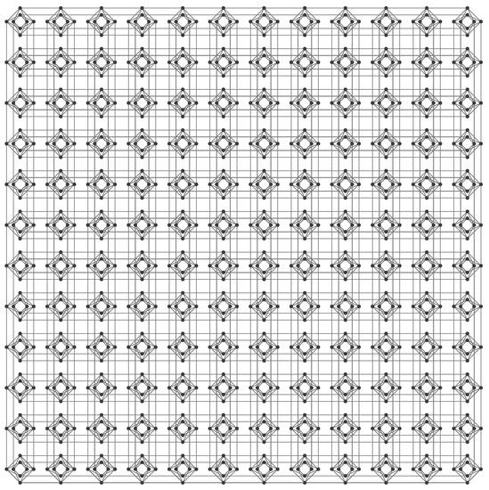
Figure 1.
The Chimera interconnection graph for the D-Wave 2X system is a array of unit cells, where each cell is a bipartite graph.
Since P is almost never a subgraph of H, P has to be minor-embedded into H, which means that each vertex of P is mapped onto a connected set of vertices (qubits) of H called chain, and the parameters of the edges (couplers) connecting the qubits in a chain are chosen so that all such qubits are getting the same value in an optimal solution, with a high probability. While this approach allows any graph P to be embedded into a sufficiently large Chimera graph H, it comes at a cost. If the Ising/QUBO problem is dense, embedding a problem of n variables requires number of qubits proportional to .
(iii) Run the annealer in order to find values of the variables producing a low energy of the quantum system modeling the Ising, which corresponds to a low value of the objective function. Due to errors caused by hardware imperfections, thermal noise, decoherence, and the short anneal times (in the order of microseconds), usually this operation is being performed many thousands of times and the best of the proposed solutions is chosen as an answer.
Since a QUBO problem cannot, by definition, contain constraints, any constraints have to be added to the objective as penalties. For instance, constraint (2) can be transformed into a penalty term that is added to the objective of a QUBO. If M is chosen large enough, then for any optimal solution the constraint (2) should be satisfied, assuming the problem is a minimization one. A drawback of such an approach is that such squared penalty will result in a QUBO or Ising with quadratic terms (nonzero coefficients ) and a complete graph P even if the original objective was sparse (with quadratic terms). Hence, our goal is to design more efficient ways to represent constraints for optimization with quantum annealers such as D-Wave.
Previous work on this problem includes [7], where the constraint embedding problem is formulated as a mixed integer optimization problem, which is solved by using MathSat solver [8], a Satisfiability Modulo Theory (SMT) [9] type solver, in a combination with using dynamic programming and exploiting the special structure of the Chimera graph. They use their algorithm to find an embedding of the Ising constraint , , producing an embedding with 8 qubits, compared to the 12 qubits required by the squared constraint penalty. However, their approach is not scalable and is restricted to problems where n is no more than 10–20 [7]. There also has been a lot of work on solving constrained optimization problems on classical computers. The approach adopted in this paper and commonly used for solving constrained problems on the D-Wave annealer belongs to the class of penalty methods, which includes barrier methods [10,11]. Another approach is the Augmented Lagrangian Method [12], which combines the penalty function with Lagrange multipliers in a single objective function. However, since the Lagrange multipliers are real numbers, the resulting problem cannot be directly solved on the D-Wave annealer, which only accepts binary variables. For further discussion of constrained methods, see [10,13,14].
For minor-embedding a general graph into the Chimera graph, Vicky Choi [15,16] show that a Chimera graph consisting of array of unit cells allows an embedding of a complete graph of vertices. Klymko et al. [17] design a polynomial-time algorithm for finding embedding of a complete graphs into a subgraph if a Chimera graph, which is relevant for the case of hardware graphs with faulty qubits and/or couplers. Boothy et al. [18] improve on that result by increasing in some case the sizes of the cliques that can be embedded and reducing the chain sizes. Cai et al. [19] design a heuristic algorithm that constructs an embedding of any graph (not necessarily clique) into the Chimera graph. Rieffel et al. [20] explore alternative ways of mapping operational planning optimization problems to QUBO problems and embedding them into the D-Wave hardware, and analyze how different mappings and parameter choices affect the effectiveness of the annealers. Bian et al. [21] develop a locally structured approach for embedding Boolean constraint satisfaction problems on the Chimera hardware and and propose decomposition algorithms for solving problems too large to fit into the hardware. Hamilton et el. [22] study what graphs can be embedded into a complete bipartite virtual hardware by defining a minor set cover (MSC), which is a is a set of minors for a given graph G, and show that the complete bipartite graph has a MSC of n minors. Goodrich et al. [23] use a graph-theoretical approach and develop an odd cycle traversal decomposition (OCT)-based embedding algorithm by exploiting the bipartite structure of the Chimera graph. Date et al. [24] propose an embedding algorithm for a Chimera graph without faults that is efficient and uses fewer qubits and produces solutions of the QUBO problem closer to the global minimum, compared to the current D-Wave embedder.
In this paper, we propose a method that allows embedding in the Chimera graph linear constraints of any number of variables. The idea of our approach is to define several patterns of variable assignments for a single cell of H, we call “tiles”, so that there is one-to-one correspondence between the variable assignments and the tilings of H. Our result implies that there exists an implementation of the constraint (2) with qubits on an -qubit Chimera graph with gap, or difference between feasible and infeasible solutions, equal to 2. Another advantage of our method is that the computation time required to compute the embedding does not depend on the number of the variables, but on the number of the tile types, so it is a constant with respect to n. Although this result implies -qubit implementation for the special case , we describe a separate algorithm with smaller constant factors.
The paper is organized as follows. In Section 2, we formally introduce the problem we want to solve and in Section 3 we present an optimization-based approach for directly solving that problem, which is however not scalable. In the next section, Section 4, we outline our proposed two-level approach that is scalable to constraints of type (2) of any size. In Section 5 and Section 6 we describe details of the implementation. Finally, in Section 7 and Section 8 we propose a better solution for the special case and describe the results of our experimental analysis. In the conclusion, we give a summary and offer some open problems.
2. Problem Formulation
Let be the set of all binary variables satisfying constraint (2) and , where . The typical implementation of the constraint (2) is as a penalty term of the type
where . Ignoring the scaling factor M, the squared difference term has the following relevant properties:
- (i)
- for each , ;
- (ii)
- for each , for some ( in this case).
Clearly, the larger the value of the parameter , which is called gap, for which (ii) is satisfied, the larger the “penalty” to the objective, if a solution to the optimization problem violates the constraint. Hence, one would like to solve the following problem:
where the QUBO problem is normalized with specific restrictions on the values of its coefficients. For such restrictions, we will use the maximum values of biases allowed on qubits and couplers by D-Wave hardware, as discussed later.
To allows values of that are better than (3), one can use ancillary binary variables and consider a quadratic binary form of both and variables of the type
to encode the constraint. Please note that linear terms and have been replaced in (5) by quadratic terms and in order to simplify notation, since the variables and are in . Then, the above optimization problem is replaced by the following one [7,25,26].
Problem 1.
Find coefficients , , and such that the QUBO problem (5) satisfies the conditions
- (C1)
- s.t. ,
- (C2)
- ,
- (C3)
- ,
Conditions (C1) and (C2) correspond to (i) and (C3) corresponds to (ii). We also take into account the physical properties of the quantum processing unit (QPU), which includes constraints on the minimum and maximum values of the coefficients , , and , which describe the range of values that the QPU hardware allows, and complying with the topology of the Chimera graph, which means that only a specific small subset of , , and coefficients are allowed to be non-zeros. Please note that while the standard penalty version (3) of the constraint does not explicitly include ancillary variables, such variables implicitly appear when is embedded in the QPU, since the embedding represents most of the variables by chains (sets) of qubits, i.e., uses extra variables. Moreover, the number of these extra (ancillary) variables grows asymptotically as the square of the problem variables, i.e., , which is very inefficient. Therefore, we will be looking for solutions in which m is a subquadratic function of n; specifically, we propose a solution where , and if k is bounded by a constant.
3. Direct Approach
We can solve (4) as an optimization problem. Conditions (C2) and (C3) can be implemented as linear constraints (since the problem variables are , , and , while and are constants), but conditions (C1) is nonlinear because of the ∃ predicate. To model (C1) as a linear constraint we define, for each , a binary vector (whose existence is guaranteed if (C1) is satisfied) and add the constraint . This creates binary variables (for ). For that number is “only” , but it grows to for and to binary variables for .
Another factor that makes the optimization problem extremely hard is that the total number of constraints is proportional to , i.e., it grows exponentially with the number of the variables. For that reason, even for , we can solve the problem only for , in reasonable time, while using the symmetry of the Chimera graph we are able to increase the size to , for . The optimal value of the gap (the parameter ) found in both cases is 4. Given that current D-Wave machines have more than thousand qubits and this number is doubling every couple of years or so, and the fact that the number of constraints grows exponentially with that number, it is clear that this approach is extremely limited in scalability and cannot handle any constraint of practical interest.
For that reason, we look for an alternative approach whose idea is to solve several optimization problems that have similar structure as the one described above, but are limited to a single cell (). Specifically, this approach has two levels. On the higher level, we define several types of cell properties that we refer to “gadgets” and a covering of the Chimera graph or a portion of it by these gadgets that will guarantee a correct solution of Problem 1 and a gap of at least 2, as long as the gadgets indeed satisfy the properties we have assumed for them. On the lower level, we show that such gadgets really exist by solving the corresponding optimization problems, which are easy because of the gadgets’ sizes.
4. A Two-Level Approach
Next, we describe a solution for arbitrary large n that uses ancillary variables. Unless stated otherwise, we consider from now on the Ising case, i.e., , since it will make it easier to establish why and how it works. Our goal is to compute the coefficients , , and as defined in (5). However, since in the Ising version for each , i.e., it is a constant, we can use (in order to avoid the introduction of new variables) the diagonal values and as coefficients for the linear terms and in the Ising problem. Hence, the Ising version of (5) is
Keys to our approach are the concepts of a gadget and a tile, discussed below, that allow any assignment of values in to the qubits of a Chimera graph to be analyzed as a geometric configuration built using several types of “tiles”, or patterns of value assignments, describing the individual unit cells of the Chimera. Depending on the types and positions of the tiles, one is able to derive the value of the Ising program for that assignment or an estimation of it, and, eventually, evidence that conditions (C1)–(C3) are satisfied. Intuitively, the difference between gadgets and tiles is that a gadget refers to the Ising coefficients of a cell, while a tile refers to a specific assignment to the variables related to a given gadget.
Next, we describe the approach in more detail. We will assume we have a fixed Chimera graph and we refer to the Ising program implementing the embedding that we are going to construct as , while its projection to a single cell c or to a set S of cells as and , respectively.
4.1. Gadgets
A gadget is an Ising program defined on variables corresponding to the qubits of a unit cell, or, equivalently, the values of the , , and coefficients of the cell. We will next describe several gadgets and, in each gadget, we are going to distinguish between three types of variables–problem, interface, and hidden variables–depending on their function. A variable can have more than one type/function. These types are the following.
- Problem variables: variables in , i.e., variables used in the original constraint (2).
- Interface variables: variables in or used for interaction and exchange of information between neighboring cells by being located on the endpoints of an edge (coupler) joining the cells.
- Hidden variables: ancillary “working” variables in used to ensure that the given gadget/tile satisfies desired properties.
We define the following three types of gadgets depending on their variables and positions in the region R of cells implementing the constraint:
- Internal gadget—for cells in the interior of R and denoted by
 ;
; - Problem gadget—containing a problem variable (and the only type that contains such a variable) and denoted by
 ;
; - Boundary gadget—for cells on the boundary of the region R of the Chimera graph implementing the constraint. The three possible orientations of this gadget will be denoted by
 ,
,  , and
, and  .
.
Figure 2a,b shows an illustration of an internal type gadget. Please note that only the four couplers denoted with red lines (the slightly longer ones in b&w) can carry information to/from the neighboring cells; the other couplers between cells will have values zero, meaning they will not be used in such implementation. A problem type gadget is illustrated on Figure 2d,e. Please note that x is both a problem and an interface variable. The boundary gadget type is similar to the problem one, except that the x variable is replaced by a t variable whose linear term takes a maximum allowed value of , forcing the variable to take value in an optimal solution. So we can think of the problem and boundary tiles as holding an x or t interface variable fixed at some value: for red, and for green.
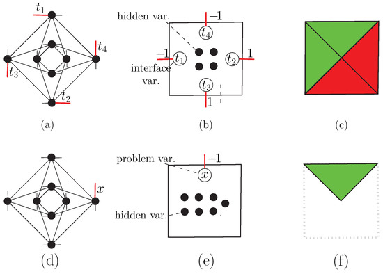
Figure 2.
Illustration of the internal () and problem () type gadgets and tiles. (a) A cell of the Chimera graph. Short lines denote couplers connecting the cell to other cells. (b) The logical structure of the corresponding internal gadget, showing the types of the variables, and, as an example, a concrete assignment of values to the interface variables. (c) The corresponding tile as used in our embedding illustrations, with red color for +1 and green for −1 type variables. Analogous illustrations for the problem type gadget and tile are found in (d–f).
) and problem () type gadgets and tiles. (a) A cell of the Chimera graph. Short lines denote couplers connecting the cell to other cells. (b) The logical structure of the corresponding internal gadget, showing the types of the variables, and, as an example, a concrete assignment of values to the interface variables. (c) The corresponding tile as used in our embedding illustrations, with red color for +1 and green for −1 type variables. Analogous illustrations for the problem type gadget and tile are found in (d–f).
4.2. Tiles
A tile is a combination of a gadget type and an assignment of values to the gadget’s variables. A tile has the same type as its corresponding gadget. Figure 2c illustrates an internal type tile and Figure 2f illustrates a problem type tile.
In addition to the interface and problem variables taking values that give the “color” of the tiles, the hidden variables also get values in . We distinguish between good and bad tiles based on both the interface and the hidden variables. In a good tile, the values of the hidden variables of the corresponding cell c have to minimize . In addition, the values of the interface variables should belong to one of several predetermined patterns. Specifically, Figure 3 illustrates all good tiles that we are going to need in order to implement the constraint (2). As in Figure 2, green corresponds to value −1 of the interface variable on the corresponding cell boundary, and red corresponds to value +1. For the problem tiles, the color also indicates the value of the corresponding problem variable x. Recall that for the good tiles, the hidden t variables are set to values that minimize the value of the cell Ising program. To denote good tile of certain type throughout the text, we will use an icon with the image of the corresponding tile as in Figure 3, e.g.,  .
.
.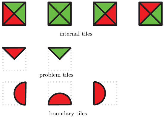
Figure 3.
The set of the good tiles.
The idea of our approach is to assign gadget types to the cells of the Chimera graph so that in any variables assignment, if all tiles are good and the interface variables between neighboring cells are consistent with each other, then that assignment minimizes , if not, then the Ising program has a value that exceeds the minimum by at least . Next we outline the procedure in more detail.
4.3. From Variables Assignments to Configurations of Tiles
Given a constraint of the type (2), determined by a pair of values , we first assign a specific gadget type to each cell of an region of cells R of the Chimera graph, and then assign values to the , , and coefficients for each cell c defined by its gadget type, resulting in an Ising program for the region R. Determining the pattern of gadgets for R and the coefficients of each gadget type will be detailed in the next sections.
Let us assume now we are given an arbitrary assignment of values to the variables in the region R. For each cell c of R, the projection of to c defines a tile that either is one of the types defined in Figure 3, or it is a bad one. Therefore, defines a unique tiling of R. Thus, instead of analyzing all possible assignments , we can study all possible tilings of R, a much smaller problem. Moreover, our gadget and tile types will be designed in such a way that analyzing the tilings of R can yield useful information about the minima of . Specifically, any tiling that consists of only good tiles and such that each tile’s adjacent tiles are in appropriate colors (good tiling) will correspond to a minimum value (optimal assignment) and, moreover, have a set of problem (x) variable values satisfying (2). On the other hand, any bad tiling (that has at least one bad tile or inconsistent colors of any pair of adjacent tiles) will have value at least above the minimum and its problem variables will violate (2). Hence, variable values satisfying (2) will produce value of the Ising program at least below the value of any problem variables violating (2).
5. Ising Program Design and Correctness Analysis
First we are going to specify the desired properties of tiles and tile pairs and then we are going to specify how to arrange the gadgets into an Ising program for the constraint.
5.1. Cost of Tiles and Tile Configurations
Consider a region of the Chimera graph consisting of a array of gadgets, an assignment of values on the variables in R, and the resulting set of tiles. The value of for is a sum of the values of all tiles in plus the sum of the values of all interactions between the tiles. Next, we set the desirable properties for the values of the tiles, depending on their type, and for their interactions.
For each tile in R, denote by the value minimized over all hidden variables. Then our requirements for the cost of are
for some constants s and , where is the gap from (C3).
To show that such tiles do exist, we will formulate and solve an optimization problem for each of the three gadget types, which will have variables the coefficients , , and restricted to a single unit cell of the Chimera graph. We will give details on the optimization problem in Section 6.
Next, we estimate the contribution of the tile interaction to . Consider a pair of adjacent tiles. Denote by the pair of the corresponding adjacent interface variables (i.e., ), by the coefficient of the corresponding quadratic term (i.e., that quadratic term is ), and by the value of that quadratic term. Please note that there are in total 4 edges joining and , but we allow only one to take a nonzero value, by setting the weights of the other 3 to zero. For any variable v, let denote the value assigned to v. Then, if we set to the maximum value of allowed by the D-Wave hardware, we have
Hence
Finally, for the cost of for , denoted by , we have
where is the set of all pairs of adjacent tiles. If all tiles in are good and all pairs in are good, we call an optimal tiling, as gets a minimum value in that case.
If is not optimal, then it will have at least one bad tile or at least one bad pair. From (6), any tiling containing a bad tile will have a value at least greater than the optimal one. Since, by (8), the difference of the values between the cases of a bad and good pair is 2, any tiling containing a bad pair will have a value by at least 2 greater than the optimal one. Hence, if is not optimal, gets a value by at least larger than the optimum.
5.2. Defining the Ising Program
To define , we assign gadgets to R as follows (see Figure 4). To all inner cells, i.e., the ones that do not share an edge on the boundary of R we assign inner gadgets. To all leftmost cells we assign positive left boundary gadgets  , to all rightmost cells we assign positive right boundary gadgets
  , and to all cells in the top row we assign positive top boundary gadgets
  . To the rest (the bottom row), we assign problem gadgets ; specifically, the i-th gadget is red, if , and green, if . The four corner cells are ignored (assigned zero coefficients). Coefficients corresponding to edges joining interface variables we set to 1, and the other coefficients we set to 0.
, to all rightmost cells we assign positive right boundary gadgets , and to all cells in the top row we assign positive top boundary gadgets . To the rest (the bottom row), we assign problem gadgets ; specifically, the i-th gadget is red, if , and green, if . The four corner cells are ignored (assigned zero coefficients). Coefficients corresponding to edges joining interface variables we set to 1, and the other coefficients we set to 0.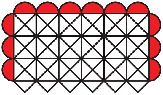
Figure 4.
Ising proram construction for the case , .
We can prove the following property characterizing feasible tilings of . If it is clear from the context, we will use R instead of to simplify notation.
Lemma 1.
There exists an optimal tiling of R and any such tiling has exactly k red problem regions.
The lemma implies that if we place the problem () variables in the problem tiles (bottom row of R), then there is a tiling of R (i.e., an assignment of the variables) that minimizes R if and only if (2) is satisfied. An example of such an optimal tiling is shown in Figure 5.
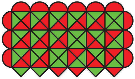
Figure 5.
Optimal tiling of .
Lemma 1 directly follows from the following property, which we prove below.
Lemma 2.
If the number of red problem tiles of R is k, then R has an optimal tiling, else R has no optimal tiling.
To prove Lemma 2, we state some properties of optimal tilings.
Proposition 1.
Any good internal tile except  ḣas opposite sides in different colors.
ḣas opposite sides in different colors.Then, in any optimal sequence of internal tiles not containing , the leftmost and the rightmost sides are of different colors. This implies that since each row of R except the first and the last one has two red boundary tiles at its ends, i.e., tiles of the same color, we have the following.
, the leftmost and the rightmost sides are of different colors. This implies that since each row of R except the first and the last one has two red boundary tiles at its ends, i.e., tiles of the same color, we have the following.Proposition 2.
In any good tiling of R, each row with internal tiles has at least one internal tile of type .
.We next prove an auxiliary lemma. Consider any row except the bottom and top ones of any optimal tiling of R and denote the corresponding Ising program as . Assume we know the colors of the top triangles of the tiles below that row (Figure 6), but we do not know the colors of the internal tiles in . Nevertheless, we will show that we can characterize the colors of the top triangles of the internal tiles of , shaded in gray in Figure 6.
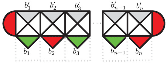
Figure 6.
A row of R, denoted by , with an assignment of values to the program variables/tiles.
Lemma 3.
The number of red colors in is exactly one less than the number of red colors in .
Proof.
By Proposition 2, there is at least one internal tile of type in . Let be the first such tile. Hence, there is no tile in and, by Proposition 1, for . Since is , is green and is red. For the remaining tiles we can see that if tile is red for , then is  , otherwise is . In both cases, . In summary, for and is red, while is green, which proves the lemma. ☐
in . Let be the first such tile. Hence, there is no tile in and, by Proposition 1, for . Since is , is green and is red. For the remaining tiles we can see that if tile is red for , then is , otherwise is . In both cases, . In summary, for and is red, while is green, which proves the lemma. ☐Lemma 3 states that the number of red colors decreases by one after each row of internal tiles in an optimal tiling, and there are k such rows, so that would prove the lemma if there is an optimal tiling. However, we do not know if such optimal tiling always exists. The next lemma helps answer when a tiling can be extended to the next row.
Lemma 4.
If there are k red tiles in , then has an optimal tiling if and no optimal tiling if .
Proof.
If , we will construct an optimal tiling explicitly. Let l be the position of the first red problem tile. Then (see the Figure 5) we define to be  , to be , and for to be if is red and , otherwise.
, to be , and for to be if is red and , otherwise.If , then all tiles in are green and we can not put a in , contradicting Proposition 2. Hence there is no optimal tiling in that case. ☐
in , contradicting Proposition 2. Hence there is no optimal tiling in that case. ☐We can now use Lemmas 3 and 4 to prove Lemma 2.
Proof of Lemma 2
Denote the j-th row of R by , where and are rows of problem and boundary tiles, respectively.
First we show that if there are red problem tiles in R, then R has an optimal tiling. Assume there are exactly k red problem tiles in . We apply Lemma 4 to and , therefore, there is an optimal tiling of and , which, by Lemma 3, has red-top triangles in (see Figure 5). Then if we apply the same argument to and and obtain that the tiling of can be extended to an optimal tiling of with number of red-top triangles in equal to . By induction, when we apply the argument to and , we conclude that the tiling of can be extended to an optimal tiling of with no red-top triangles in . Since all top triangles in are green, they are consistent with respect to their colors with the boundary triangles in , implying that we have an optimal tiling of the entire R.
Now assume that the number of red problem tiles in R is not k. If , then, by the first part of the proof, will contain a red-top triangle which will create a mismatch with an adjacent red boundary tile in . If , then the tiling of would not be extendible to an optimal tiling of , since would have no red-top tile and, hence, cannot contain , which tile is required in by Proposition 2 in any optimal tiling. Hence, there is no optimal tiling of R if . ☐
, which tile is required in by Proposition 2 in any optimal tiling. Hence, there is no optimal tiling of R if . ☐6. Solving the Optimization Problem
For each gadget type, we need to define a single-cell Ising program so that conditions (6) are satisfied for all possible tiles for that gadget, and the value of the gap parameter is maximized. We will give details for the internal gadget since it is the most interesting. For this gadget, we have 4 good tiles , , , and , and all others are bad tiles. Denote this Ising program by and its coefficients by (since internal gadgets do not have variables, their coefficients in front of the and terms are zeros). Define sets of all 4-tuples of interface variables of good internal tiles (see Figure 2) and of all remaining 4-tuples. Then we formulate the following optimization problem.
since it is the most interesting. For this gadget, we have 4 good tiles , , , and , and all others are bad tiles. Denote this Ising program by and its coefficients by (since internal gadgets do not have variables, their coefficients in front of the and terms are zeros). Define sets of all 4-tuples of interface variables of good internal tiles (see Figure 2) and of all remaining 4-tuples. Then we formulate the following optimization problem.Problem 2.
Find values for the coefficients and parameters μ and γ such that satisfies the conditions
- (C1)
- For all s.t. ,
- (C2)
- For all ,
- (C3)
- For all
and γ is maximized.
This is the same type of problem as Problem 1, but of much smaller size. We model Problem 2 as a mixed-integer programming (MIP) problem. We replace each variable by a binary variable using the linear transformation . Since is linear with respect to variables , conditions (C2) and (C3) of Problem 2 can be easily encoded as linear constraints. To encode condition (C1), we introduce, for each , new binary variables , corresponding to the values from condition (i). This introduces binary variables. Then (C1) is replaced by
This removes the ∃ predicate, but since the Ising program coefficients are variables, the resulting constraint is cubic (there are cubic terms of the type ).
We linearize each such product by introducing a new real variable and adding the constraints
and we use a similar technique to linearize quadratic terms of the type , where is real and is binary.
We implemented Problem 2 using the AMPL modeling language [27] and the Gurobi solver [28]. The resulting linear program has 16 binary variables, 234 continuous variables, and 884 constraints. Gurobi found the optimal solution in a tiny fraction of a second, with and . Please note that a value would have been sufficient, since the penalty for mismatched adjacent tiles is only 2 and the gap for the entire Ising program is the minimum of the gap between good and bad tiles and the gap between good and bad tile pairs.
Corollary 1.
The Ising program defined in Section 5 is a solution of Problem 1 with .
7. Improved Embeddings for the Case
In this section, we are going to describe better embeddings for the case , i.e., when the number of variables should be one.
7.1. Reducing the Number of Cells
While, for the case , we can use the embedding described in the previous sections, that embedding is going to use Chimera graph cells and the maximum n is restricted by the number of cells in one row of the Chimera graph, which for the case of D-Wave 2X is 12 and for D-Wave 2000Q is 16. In this section, we describe an embedding for the case of , i.e., of the constraint
using just (one row of) cells. We will later show how we can extend the embedding to cover all the cells of the Chimera graph.
The type of the variables are the same as in the general case, i.e., problem, interface, and hidden variables. However, now we have only the following two types of gadgets:
- An internal gadget—for cells in the interior of the row, and will be denoted by
 . Each internal gadget contains one problem, two interface, and five hidden variables (Figure 7a,b).
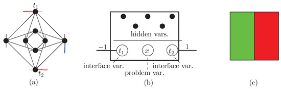 Figure 7. Illustration of the internal type gadgets and tile for the case . (a) A cell of the Chimera graph. Short lines indicate the couplers connecting to the neighboring cells (some may be missing for boundary cells). (b) The logical structure of the the corresponding internal gadget. There are two edges (couplers) shown in red (thicker line in b&w) in (a) with weights (in he example) and 1 connecting it to the neighboring cells in the row. The coupler shown in blue, in combination with the red coupler on top, is used in the gadget discussed in Section 7.2. (c) The corresponding tile as used in our embedding illustrations, with red color for +1 and green for −1 type variables.
 - A boundary gadget—for cells on the two ends of the row. They are similar to the boundary gadgets in the general case, but come in only two orientations, which will be denoted by and .
As in the previous case, tiles are gadgets with assignments of values in to their variables and have the same type as their corresponding gadgets. The values of the interface variables are used to assign colors to the corresponding halves of the tile in our notation, where green corresponds to value −1 and red corresponds to value +1. An internal tile corresponding to the gadget on Figure 7b is shown on Figure 7c. The set of all good tiles is illustrated on Figure 8. Recall that in order for a tile to be good, it should have a combination of program and interface variables as shown on Figure 8 and values of the hidden variables that minimizes the corresponding cell Ising program. Note also that (only) the  tile has value of the x variable set to 1 and the other two good tiles hold an x variable set to .
tile has value of the x variable set to 1 and the other two good tiles hold an x variable set to .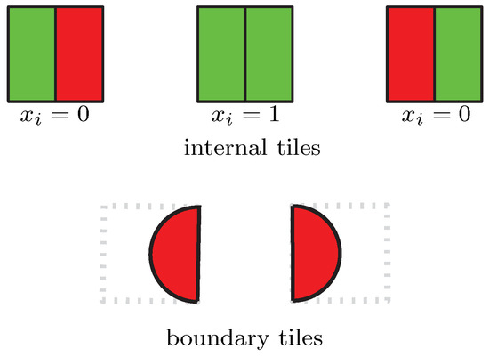
Figure 8.
The set of the good tiles for the case .
The cost of the tiles and configurations of tiles is defined in the same way as in the previous sections, i.e., using (6), (8) and (9). Similarly, we define a good tiling as a tiling all of whose tiles and tile pairs are good.
We next define an Ising program for implementing the constraint (10) corresponding to the gadget configuration shown on Figure 9a, i.e., such that it covers a row or a sub-row of cells, and has n internal gadgets plus two boundary gadgets on the ends. We want to show that the minimum cost of a tiling of (Figure 9b) corresponds to an assignment to the x variables that has exactly one x variable, which is equivalent to an optimal tiling containing exactly one tile. To estimate the value of , we state the following analogues of Propositions 1 and 2.
tile. To estimate the value of , we state the following analogues of Propositions 1 and 2.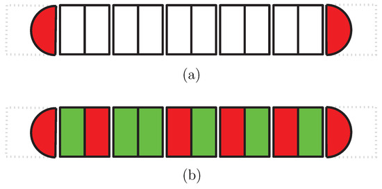
Figure 9.
(a) Ising program for the case , . (b) The structure of an optimal tiling of . In such tiling, adjacent halves of neighboring tiles should be in different colors.
Proposition 3.
Any good internal tile except ḣas left and right sides in different colors.
ḣas left and right sides in different colors.Proposition 4.
Since the end tiles of are in red, in any good tiling of there is at least one tile.
tile.From Proposition 4, any good tiling corresponds to an assignment to the x variables with at least one value. On the other hand, it can be easily observed that a good tiling cannot have more than one green tiles. Indeed, consider the position i of the first . On position , we should have a tile with a left side colored in red, which cn be either a or a  tile. In the former case, the tile on the i-th position is the last internal tile from the left, so it is the only tile. In the latter case, a tile has a right side in green, so it can be followed by either a or a tile. By induction, it follows that the first tile is followed by tiles and a tile. Hence we have the following analogue of Lemma 1.
. On position , we should have a tile with a left side colored in red, which cn be either a or a tile. In the former case, the tile on the i-th position is the last internal tile from the left, so it is the only tile. In the latter case, a tile has a right side in green, so it can be followed by either a or a tile. By induction, it follows that the first tile is followed by tiles and a tile. Hence we have the following analogue of Lemma 1.Lemma 5.
There exists an optimal tiling of if and only if there is exactly one x variabe set to .
Solving the optimization problem needed to find the coefficients , , and for the Ising program corresponding to an internal gadget is done as in Section 6. If we identify each tile by the set of program and interface variables as in Figure 8, the sets good and bad tiles can be explicitly defined as
Then the optimization problem is formulated and solved exactly as in Section 6, finding an optimal solution with with and . Since the gap for the entire Ising program is the minimum of the gap between good and bad tiles, which is 4, and the gap between good and bad tile pairs, which with with one active edge coupler (i.e., with non zero weight) is 2, we have the following result.
Corollary 2.
7.2. Increasing the Size of the Constraint
In the previous subsections, we only showed how to embed constraints using Chimera graph cells, almost three times fewer than with the general approach. However, since our design uses a single row of cells, it means that on a (-grid Chimera graph we could only embed a constraint with variables, or 10 variables in case of D-Wave 2X and 14 variables in case of D-Wave 2000Q. We now show that we can easily adapt the above approach to use all the unit cells of the Chimera graph, allowing us to be able to embed constraint with up to variables.
The reason we were restricted to a single row in the previous design was that we used only horizontal edges (couplers) to connect to the neighboring cells (Figure 7). Hence, in order to allow such sequences to occupy more than one row, we need to define “corner” tiles that have combinations of horizontal and vertical connecting edges and thereby allow “turns”, and use them together with the tiles defined for the single-row case to produce snake-like configurations of the type illustrated on Figure 10.
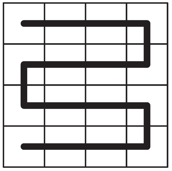
Figure 10.
This example illustrates the connections between the tiles in a solution for the multi-row case for a Chimera graph of size cells, each cell representing a tile with one problem variable, with the exception of first and last tiles that contain no problem variables.
Therefore, we have to introduce “corner” analogues of the “straight” tile types from Figure 7. The only difference between the new and old tiles is the positions of the type variables, which for the new types should be on one row and one column of the Chimera graph cell. On Figure 7a, the top red and the side blue edges illustrate the positions of the interface variables for a corner tile allowing a clockwise turn.
To find the , , and coefficients for the new gadgets, we have to solve a similar but different optimization problem compared to the one described in Section 6, for the new gadgets only. We map the variables as illustrated on Figure 11. Implementing the optimization problem in AMPL and solving it with the Gurobi solver, we find and .
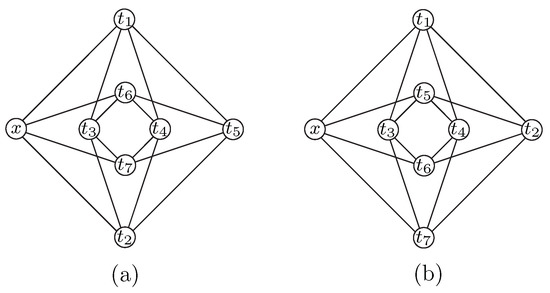
Figure 11.
Positions of the x and t variables in a Chimera graph cell for the optimization problem (a) in the single-row embedding, and (b) for the extra gadgets in the multi-row embedding.
Please note that we do note need to compute different sets of gadgets for clockwise and counterclockwise turns because of the symmetries in the Chimera graph cell. Although the values of , , and are generally different for clockwise and counterclockwise turns, they can be converted from one into the other by suitable permutations of the variable positions.
7.3. Increasing the Gap
Here we show that with an approach similar to the one described in the previous subsections one can increase the gap from two to four.
Recall that the gap between good and bad tiles in all previous implementations was already four, but, because the gap between good and bad tile pairs was two due to adjacent gadgets being connected by a single edge, the gap for the entire constraint was also .
To increase the gap to four, it will be enough to add additional connecting edges between consecutive cells. In particular, instead of one edge between cells/tiles, we now want to use two edges, which would double the gap between good and bad pairs. With such a design, we have four interface variables per cell/gadget (two of which are connected to the previous cell and two connected to the next one) and we have only three hidden variables, see Figure 12. Therefore, we have a new optimization problem with sets
described as 5-tuples of interface and problem variables , and
containing the remaining 5-tuples. Notice, that for all elements in , we have and , so in order to get the new good tile types from the old ones (conceptually) we just need to duplicate pairs into pairs . Except for the redefinition of the sets, the optimization program remains the same. Using Gurobi, we found the coefficients for the constraint embedding with and .
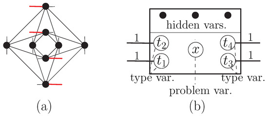
Figure 12.
The structure of the tiles for the case of . (a) A cell of the Chimera graph. Short lines indicate the couplers connecting to the neighboring cells. (b) The logical structure of the tile corresponding to that cell. Edges correspond to couplers shown in red in (a).
In the next section, we discuss implementation and experimental results.
8. Experiments
We performed some experiments in order to validate our constraint embedding algorithm and to evaluate the properties of the embeddings. We experimented with the case since it allows larger problems to be embedded and because that design is less sensitive to faults in the D-Wave hardware. Due to errors during manufacturing and calibration, only 1095 qubits and 3061 couplers out of 1152 and 3360, respectively, are operational on the D-Wave 2X machine available at Los Alamos, where we did all experiments. We test the multi-row and increased-gap algorithms described above as most interesting.
8.1. Multi-Row Algorithm
As mentioned above, the Chimera graph for Los Alamos’ machine (as well as all other D-Wave machines manufactured so far) lack some vertices/qubits and edges/couplers. This creates a problem for using our embedding algorithm, which assumes each Chimera graph cell has all 8 vertices and 16 edges and that certain edges between cells also exist.
8.1.1. Embedding in the Real Chimera Graph
We first sketch our approach to deal with imperfect Chimera graphs. The main idea is that we use only cells that are complete (meaning they have maximum number of vertices and edges) to represent gadgets, while all other (incomplete) cells are only used for interconnecting perfect ones. Specifically, if we have two complete cells and that are separated by one or more faulty cells, and need to connect interface variable from with interface variable from (see Figure 7), we create a “chain” between and from qubits from the faulty cells, with interconnecting couplers between qubits set to , thereby forcing all qubits on the chain to get the same value. (A similar idea of constructing chains is used to minor-embed graphs representing general QUBO problems into the Chimera graphs.) For instance, Figure 13 shows two perfect cells and with one faulty cell between them. The coefficients , , and of and are set to the values determined from the solution of the optimization problem from Section 6. To connect the variable of (top of ), denoted by , to the type variable of (top of ), denoted by , the weights on the edges/couplers of as well as the edge connecting to are set to , forcing all variables in to take, in a minimum-energy solution, the same values as . Hence, this type of a connection has the same effect as connecting directly to .
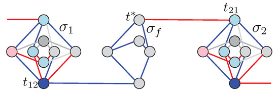
Figure 13.
Figure illustrating a connection between two perfect cells by a chain of bad-cell vertices and edges. Colors on the vertices and edges encode the values of the corresponding coefficients, where blue is for negative, red for positive, and gray is for near-zero, and the intensities of colors encode the magnitudes. The couplers of cell are all set to forcing and to take the same values in an optimal solution.
With this simple approach, we were able to embed the constraint (10) for , see Figure 14. (Please note that some faulty cells have all eight qubits but miss one or more couplers, which cannot always be seen in the figure’s resolution.) We want next to test how certain parameters of the approach affect the quality of the embedding.
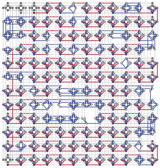
Figure 14.
Embedding of the Ising constraint (corresponding to QUBO constraint ) for . Colors encode vertex and edge values as in Figure 13.
8.1.2. Analysis
We performed two experiments. In the first experiment, we analyze whether and how the accuracy of the solution is affected by the value of the gap parameter . While the constraint (10) should be satisfied for any values of and minimizing the quadratic Ising program (5), for a solution returned by the D-Wave machine that may not be necessarily true due to the annealer’s stochastic behavior. The reason is that, because of incoherence, flux noise, background susceptibility, etc. [29], the D-Wave machine might not be able to find the global minimum of the Ising program implementing the constraint, and hence the constraint may not be satisfied. Because of such inherent inaccuracy, when solving NP-hard optimization problems one usually performs thousands of anneals on the same input and chooses the best result as a solution. This is justified as annealing and comparing the results is relatively fast, while coming with good candidate solutions in the case of NP-hard problems is very difficult.
Therefore, one would expect that for greater , i.e., when the difference between the global minimum and the best suboptimal solutions is greater, it would be easier for the D-Wave machine to distinguish between optimal and suboptimal solutions, and therefore the accuracy would also be better.
To produce embeddings with different values for , we modify the solution described above. Recall the value of the gap of is determined as the minimum of the gap between the good and bad tiles, which is four, and the gap between good and bad pairs of tiles, which is two. Recall also that the second type of gap is equal to twice the absolute value of the bias (weight) on the coupler (edge) between the adjacent cells, which absolute value is . Hence, if we change in the weight of each interface edge between cells, currently set at , to a weight , this will result in an embedding with . In this way, one can generate a set of embeddings with arbitrary values for between 0 and 2.
Figure 15 shows results based on the embedding illustrated on Figure 14 modified with respect to as discussed above. In all experiments in this section, the results are for 10,000 anneals averaged over 10 trials. Each curve, shown in a different color, corresponds to an embedding with a given value of the parameter , ranging from 0.2 to 2. The quantity we measure is the number of problem variables with value . As we can expect, the larger the gap , the better the embedding (curves that are to the left correspond to better embeddings). However, even the best embedding, for , is still of insufficient quality. That raises the question whether other parameters such as the number of problem variables can also affect the quality of the embedding.
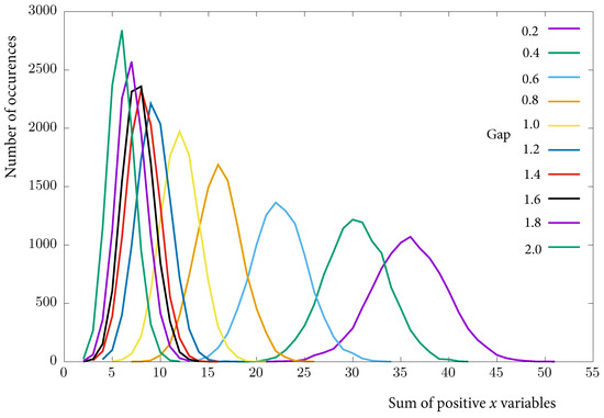
Figure 15.
Dependence of the quality of the constraint embedding measured as the value of the sum of all (horizontal axis) on the value of the gap parameter, shown as curves of different colors. The vertical axis shows the frequency, or how many times, out of 10,000, the solution returned by the D-Wave annealer had the respective sum.
In the second experiment, we study how the accuracy of the solution depends on the size of the problem vector x (the value of the size parameters n). For this purpose, for each number of variables q in , we modify the embedding from Figure 14 by including the first q perfect cells (as well as the connecting imperfect cells between them to keep the connectivity) and then also adding the last cell (which corresponds to a boundary gadget). Then we submit the corresponding Ising problems to the D-Wave annealer. The results are displayed on Figure 16. They show that increasing the number of problem variables has an effect on the quality of the results by increasing the number of values in the solution, although the decrease in quality is not so great as in the previous experiment. Our hypothesis about why the length of the x vector has an effect on the quality is that, because of the short annealing time for the D-Wave annealer, information does not have enough time to travel from one end of the “snake” from Figure 10 to the other. Hence, the D-Wave annealer does not have time to “see” the entire sequence of tiles and produces a solution that consists of several locally optimal subsequence of length about 10 each that satisfy the constraint, i.e., have exactly one x variable with value in them.
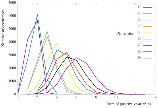
Figure 16.
Dependence of the quality of the constraint embedding on the length of the vector x (number of problem variables ). Results for sizes are shown in different colors.
The results of the experiments point to two possible ways to improve the embedding algorithm: increasing the gap and decreasing the diameter (the maximum distance between any two vertices in the embedding). While decreasing the diameter is an interesting open problem, in the next section we discuss results on using increased gap, i.e., using the algorithm from Section 7.3.
8.2. Increased-Gap Algorithm
We first discuss how we modify the original embedding to take into account the defective Chimera graph cells and then discuss experimental results.
8.2.1. Modifying the Embedding for the Real Chimera Graph
Because of the large number of defects in the Chimera graph, it is not feasible to use same approach as in Section 8.1 to connect nearest complete cells using the faulty ones between them, as we now need to have two independent edges between adjacent perfect cell. The algorithm we use in this case finds all perfect cells of the real Chimera graph and constructs a graph as the subgraph of the real Chimera graph induced by the vertices of the perfect cells. We also define a graph , where we contract each cell of into a single vertex and put an edge between two vertices representing cells and , if the two edges needed to connect and exist in . Ideally, now we need to solve a longest path problem, i.e., to find a longest path in , which is an NP-hard problem. This path would then define cells that can be used to embed our constraint.
However, because our focus is not on solving the longest path problem, a challenging problem in itself, we manually handpick such a path in , and, as one can see from Figure 17, the handpicked path still has a reasonable length (84, down from 92 in the previous case), and therefore leads to dimensionality of 82, as we use the first and last cells for boundary gadgets.
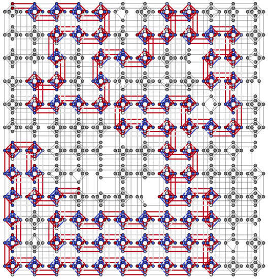
Figure 17.
Illustration of our implementation for a vector x with 82 coordinates on a real D-Wave 2X hardware, which vector is constrained to contain exactly one coordinate.
Again, as in the multi-row case from the previous section, we have to introduce new type of gadgets that allow us doing “turns”, as in Figure 10. In this particular case, we have a total of 3 types of gadgets related to “turns”, specifically, (i) horizontal (adjacent cells are both either on the same row or on the same column; the same type used in the single-row case), (ii) clockwise (adjacent cells’ positions form a 90° angle in clockwise direction), (iii) counterclockwise (adjacent cells’ positions form a 90° angle in counterclockwise direction). We are not going into details as the formulation of this optimization problems is analogical to the previous ones, the difference being only in the position of the type variables in the cell. See Figure 17 for the resulting implementation.
8.2.2. Results
We performed an experiment similar to the experiment from the previous two subsections, where we track the number of coordinates in the solution vector and how that number depends on the dimensionality of the vector. We tried dimensions (in this case we have only 80 instead of the 90 variables in the previous one, since the largest dimension we were able to embed now is only 82), see Figure 18. For each case we do batches of 10,000 anneals and show averaged results over 10 runs. The results indicate that now the accuracy is much better since the largest sum is 5, down from 10 in Figure 16. Moreover, in 4 cases (out of 8) we now have more than 5000 instances with the correct sum, while on Figure 16 the highest score is about 4000. Also, for the shortest vector (dimension 10), we have near 100% correct results (9999 correct out of 10,000).
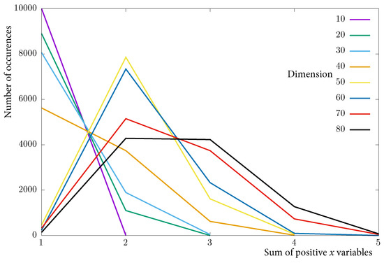
Figure 18.
In this figure one can see how the dimension of affects the accuracy of the embedding of the constraint, i.e., the number of s in the resulting vector.
9. Using the Constraint Embeddings for Solving Constrained Optimization Problems
In the previous sections, we focused on finding an embedding of a single constraint in the Chimera graph. An interesting question is whether the proposed solution can be combined with an embedding of an objective function and possibly with other constraints in the Chimera graph in order to solve quadratic binary constrained problems. The difficulty is that the placement of the problem variables x in the constraints and in the objective function embeddings may be inconsistent with each other. Connecting different copies of the same variable by chains in order to force them to take the same value is likely to be very expensive in terms of qubit usage and may even be impossible. To resolve this issue, we offer a different approach that makes use of the constructed Ising program implementing the constraint, but ignores the mapping of variables to specific vertices of the Chimera graph details. Although we are not using the mapping, we are still making use of the sparsity of the Chimera graph, which is preserved in the Ising program of the embedding.
The proposed approach involves the following three steps. (i) Find an Ising program for the constraint using the method described in the previous sections. The only difference is that one can use now a complete graph instead of a bipartite one for the unit cell or change the size of the cells, in order to get a better gap or to use fewer variables. (ii) Add together the Ising program of the constraint(s) and the Ising program of the objective, using appropriate weights. (iii) Embed the resulting Ising problem onto the Chimera graph using any embedder, e.g., the one offered by D-Wave. While we lose the advantage of having the Ising program of the constraint already embedded onto the target hardware, the other two advantages, sparsity of the Ising program and a bigger gap, still remain. Fine-tuning the parameters and experimentally analyzing such an approach can be a subject of further research.
10. Conclusions
We described an optimization-based approach that allows implementing linear constraints of the type (2) using ancillary variables and achieving gap two. Moreover, the resulting Ising has structure that is consistent with the Chimera graph, i.e., allows each variable to be mapped to a single qubit. When k gets close to n, then our algorithm has the same complexity with respect to the number of the quadratic terms (which translates to the number of qubits needed) as the standard penalty implementation (3). When , then our algorithm uses asymptotically optimal number of qubits. In the special case , we design an improved algorithm that uses approximately three times fewer qubits and has twice bigger gap between feasible and infeasible solutions. Our experiments confirmed that maximizing the gap is a meaningful quality criterion objective. Our work raises several open problems for future research such as finding ways to better embed constraints for real Chimera graphs taking into account the faulty qubits and couplers, and developing embedding methods that results in smaller diameters (the largest distance between qubits in the embedding using paths of active/nonzero couplers).
Author Contributions
T.V. developed some main ideas and did most of the programming and experimental analysis. H.D. formalized the proofs and drafted the manuscript. Both authors had multiple discussions on all aspects of the work, provided critical feedback of the manuscript, read and approved the final manuscript.
Funding
Research presented in this article was supported by NSF grant 1514164 AF and by the Laboratory Directed Research and Development program of Los Alamos National Laboratory under project numbers 20180267ER and 20190065DR. This work was also supported by the U.S. Department of Energy through Los Alamos National Laboratory. Los Alamos National Laboratory is operated by Triad National Security, LLC for the National Nuclear Security Administration of the U.S. Department of Energy (contract no. 89233218CNA000001).
Conflicts of Interest
The authors declare no conflict of interest.
References
- Garey, M.R.; Johnson, D.S. Computers and Intractability: A Guide to the Theory of NP-Completeness; W. H. Freeman & Co.: New York, NY, USA, 1979. [Google Scholar]
- Sahni, S. Computationally Related Problems. SIAM J. Comput. 1974, 3, 262–279. [Google Scholar] [CrossRef]
- Johnson, M.; Amin, M.; Gildert, S.; Lanting, T.; Hamze, F.; Dickson, N.; Harris, R.; Berkley, A.; Johansson, J.; Bunyk, P.; et al. Quantum annealing with manufactured spins. Nature 2011, 473, 194–198. [Google Scholar] [CrossRef] [PubMed]
- Bunyk, P.; Hoskinson, E.; Johnson, M.; Tolkacheva, E.; Altomare, F.; Berkley, A.; Harris, R.; Hilton, J.; Lanting, T.; Przybysz, A.; et al. Architectural Considerations in the Design of a Superconducting Quantum Annealing Processor. IEEE Trans. Appl. Supercond. 2014, 24, 1–10. [Google Scholar] [CrossRef]
- Lucas, A. Ising formulations of many NP problems. Front. Phys. 2014, 2, 1–27. [Google Scholar] [CrossRef]
- Bichot, C.; Siarry, P. Graph Partitioning; Wiley-IST: Hoboken, NJ, USA, 2013. [Google Scholar]
- Bian, Z.; Chudak, F.; Israel, R.; Lackey, B.; Macready, W.G.; Roy, A. Discrete optimization using quantum annealing on sparse Ising models. Front. Phys. 2014, 2, 56. [Google Scholar] [CrossRef]
- Cimatti, A.; Griggio, A.; Schaafsma, B.J.; Sebastiani, R. The MathSAT5 SMT Solver. In Tools and Algorithms for the Construction and Analysis of Systems; Piterman, N., Smolka, S.A., Eds.; Springer: Berlin/Heidelberg, Germany, 2013; pp. 93–107. [Google Scholar]
- De Moura, L.; Bjørner, N. Satisfiability Modulo Theories: Introduction and Applications. Commun. ACM 2011, 54, 69–77. [Google Scholar] [CrossRef]
- Bertsekas, D. Nonlinear Programming; Athena Scientific: Nashua, NH, USA, 1999. [Google Scholar]
- Auslender, A.; Cominetti, R.; Haddou, M. Asymptotic Analysis for Penalty and Barrier Methods in Convex and Linear Programming. Math. Oper. Res. 1997, 22, 43–62. [Google Scholar] [CrossRef]
- Birgin, E.; Martínez, J. Practical Augmented Lagrangian Methods for Constrained Optimization; Society for Industrial and Applied Mathematics: Philadelphia, PA, USA, 2014. [Google Scholar] [CrossRef]
- Chong, E.K.P.; Zak, S.H. Algorithms for Constrained Optimization. In An Introduction to Optimization; Wiley-Blackwell: Hoboken, NJ, USA, 2011; Chapter 22; pp. 513–539. [Google Scholar] [CrossRef]
- Kochenberger, G.; Hao, J.K.; Glover, F.; Lewis, M.; Lü, Z.; Wang, H.; Wang, Y. The Unconstrained Binary Quadratic Programming Problem: A Survey. J. Comb. Optim. 2014, 28, 58–81. [Google Scholar] [CrossRef]
- Choi, V. Minor-embedding in adiabatic quantum computation: I. The parameter setting problem. Quantum Inf. Process. 2008, 7, 193–209. [Google Scholar] [CrossRef]
- Choi, V. Different adiabatic quantum optimization algorithms. Quantum Inf. Comput. 2011, 11, 638–648. [Google Scholar]
- Klymko, C.; Sullivan, B.D.; Humble, T.S. Adiabatic quantum programming: Minor embedding with hard faults. Quantum Inf. Process. 2014, 13, 709–729. [Google Scholar] [CrossRef]
- Boothby, T.; King, A.; Roy, A. Fast clique minor generation in Chimera qubit connectivity graphs. Quantum Inf. Process. 2016, 15, 495–508. [Google Scholar] [CrossRef]
- Cai, J.; Macready, W.G.; Roy, A. A practical heuristic for finding graph minors. arXiv, 2014; arXiv:1406.2741. [Google Scholar]
- Rieffel, E.G.; Venturelli, D.; O’Gorman, B.; Do, M.; Prystay, E.M.; Smelyanskiy, V. A case study in programming a quantum annealer for hard operational planning problems. Quantum Inf. Process. 2015, 14, 1–36. [Google Scholar] [CrossRef]
- Bian, Z.; Chudak, F.; Israel, R.B.; Lackey, B.; Macready, W.G.; Roy, A. Mapping Constrained Optimization Problems to Quantum Annealing with Application to Fault Diagnosis. Front. ICT 2016, 3, 14. [Google Scholar] [CrossRef]
- Hamilton, K.E.; Humble, T.S. Identifying the minor set cover of dense connected bipartite graphs via random matching edge sets. Quantum Inf. Process. 2017, 16, 94. [Google Scholar] [CrossRef]
- Goodrich, T.D.; Sullivan, B.D.; Humble, T.S. Optimizing adiabatic quantum program compilation using a graph-theoretic framework. Quantum Inf. Process. 2018, 17, 118. [Google Scholar] [CrossRef]
- Date, P.; Patton, R.; Schuman, C.; Potok, T. Efficiently embedding QUBO problems on adiabatic quantum computers. Quantum Inf. Process. 2019, 18, 117. [Google Scholar] [CrossRef]
- Vyskocil, T.; Djidjev, H. Simple constraint embedding for quantum annealers. In Proceedings of the International Conference on Rebooting Computing, Tysons, VA, USA, 7–9 November 2018. [Google Scholar]
- Vyskocil, T.; Pakin, S.; Djidjev, H. Embedding Inequality Constraints for Quantum Annealing Optimization; Technical Report LA-UR-18-3097; Los Alamos National Laboratory: Alamos, NM, USA, 2018.
- Fourer, R.; Gay, D.M.; Kernighan, B.W. AMPL: A Modelling Language for Mathematical Programming, 2nd ed.; Cengage Learning: Boston, MA, USA, 2002. [Google Scholar]
- Gurobi Optimizer Reference Manual; Gurobi Optimization, Inc.: Beaverton, OR, USA, 2015.
- Technical Description of the D-Wave Quantum Processing Unit; 09-1109A-A; D-Wave: Burnaby, BC, Canada, 2016.


© 2019 by the authors. Licensee MDPI, Basel, Switzerland. This article is an open access article distributed under the terms and conditions of the Creative Commons Attribution (CC BY) license (http://creativecommons.org/licenses/by/4.0/).