Heterogeneous Distributed Big Data Clustering on Sparse Grids

Abstract

Clustering is an important task in data mining that has become more challenging due to the ever-increasing size of available datasets. To cope with these big data scenarios, a high-performance clustering approach is required. Sparse grid clustering is a density-based clustering method that uses a sparse grid density estimation as its central building block. The underlying density estimation approach enables the detection of clusters with non-convex shapes and without a predetermined number of clusters. In this work, we introduce a new distributed and performance-portable variant of the sparse grid clustering algorithm that is suited for big data settings. Our computed kernels were implemented in OpenCL to enable portability across a wide range of architectures. For distributed environments, we added a manager–worker scheme that was implemented using MPI. In experiments on two supercomputers, Piz Daint and Hazel Hen, with up to 100 million data points in a ten-dimensional dataset, we show the performance and scalability of our approach. The dataset with 100 million data points was clustered in 1198$\mathrm{s}$ using 128 nodes of Piz Daint. This translates to an overall performance of 352 $\mathrm{TFLOPS}$. On the node-level, we provide results for two GPUs, Nvidia’s Tesla P100 and the AMD FirePro W8100, and one processor-based platform that uses Intel Xeon E5-2680v3 processors. In these experiments, we achieved between 43% and 66% of the peak performance across all computed kernels and devices, demonstrating the performance portability of our approach.

1. Introduction

In data mining, cluster analysis partitions a dataset according to a given measure of similarity. The partitions obtained as a result of the clustering process are called clusters. The clustering of big datasets poses additional challenges as not all clustering algorithms scale well in the size of the dataset. Furthermore, mapping clustering approaches to modern hardware platforms such as graphics processing units (GPUs) requires new parallel approaches. And for the use on supercomputers or in the cloud, algorithms need to be designed for distributed computing.

There is a wide range of algorithms that perform clustering. The classic k-means algorithm iteratively improves an initial guess of cluster centers [1]. Efficient variants of the k-means algorithm have been proposed, e.g., by using domain partitioning through k-d-trees [2] or by a more careful selection of the initial cluster centers [3]. As a major disadvantage, k-means requires the number of clusters to be known in advance, which is not always possible. Moreover, in contrast to many alternatives, k-means cannot detect clusters with non-convex shape.

DBSCAN probably is the most widely used density-based clustering approach [4]. In its basic form, it constructs a cluster based on the number of data points in an $ϵ$-sphere around each data point. If spheres overlap and have enough data points in them, the data points are part of the same cluster. For m data points, the complexity of DBSCAN was stated as $\mathcal{O}(mlogm)$ in the original paper [4]. However, more recent work shows that the actual complexity has a lower bound of $\Omega \left(m^{4/3}\right)$ [5,6].

DENCLUE is another example for clustering based on density estimation. It uses a kernel density estimation algorithm [7]. Spectral clustering methods cluster datasets by solving a mincut problem on a weighted neighborhood graph [8]. There are many more approaches to clustering, e.g., using neural networks [9], described in the literature [1,10].

Some clustering algorithms support GPUs for higher performance. Takizawa and Kobayashi presented a distributed and GPU-accelerated k-means implementation in 2006, before modern GPGPU frameworks like CUDA and OpenCL were available [11]. Since then, further GPU-enabled k-means algorithms have been developed [12,13,14,15]. Fewer published results are available for density-based GPU-accelerated clustering. CUDA-DClust is a GPU-accelerated variant of DBSCAN that uses an indexing approach to reduce distance calculations [16]. Andrade et al. developed a GPU-accelerated variant of DBSCAN called G-DBSCAN employing an algorithm with quadratic complexity in the dataset size [17].

While many clustering algorithms have been proposed, not many have been shown to work in big data scenarios. k-means++ is a map-reduce variant of the k-mean algorithm that has been used to cluster a $4.8$ million data points dataset on a Hadoop cluster with 1968 nodes [18]. MR-DBSCAN is a DBSCAN variant that could cluster a 2-D dataset with up to $1.9$ billion data points and is implemented with a map-reduce approach as well [19]. The published results of MR-DBSCAN demonstrate excellent performance. However, it uses a grid discretization that makes assumptions on the distribution of the dataset throughout the domain. Furthermore, it is unclear how the algorithm will scale to higher dimensions, as the grid discretization is fully affected by the issue of dimensionality [20]. RP-DBSCAN implements a similar approach compared to MR-DBSCAN, but uses a more advanced partitioning scheme [5]. RP-DBSCAN was able cluster a 13-D dataset with $4.4$ billion data points.

In this work, we introduce a new distributed and performance-portable variant of the sparse grid clustering algorithm. This approach builds upon prior work which presented the basic theory and compared our approach to other clustering strategies [21].

The unique building block of our approach is the sparse grid density estimation algorithm. Sparse grids are a method for spatial discretization that has been applied to higher-dimensional settings with up to 166 dimensions and moderate intrinsic dimensionality [22]. Therefore, in contrast to many spatial partitioning approaches, the underlying sparse grid density estimation mitigates the issue of dimensionality. The sparse grid clustering method does not rely on assumptions about the distribution of data; it can successfully suppress noise and it can detect clusters of non-convex shape. Compared to k-means, sparse grid clustering does not require the number of clusters as a parameter of the algorithm. In this paper, we use the Euclidean norm as the measure for the similarity of data points.

Methods based on sparse grids have been used for regression and classification tasks [22,23]. In prior work, we have shown the applicability of these methods in heterogeneous computing and high-performance computing settings [24,25,26]. However, to our knowledge this work presents the first high-performance results for sparse grid clustering.

Our algorithm was designed with a focus on high performance and performance portability. On the node-level we use OpenCL, as it offers basic portability across a wide range of hardware platforms. We not only support GPUs and processors of different vendors, our approach achieves a major fraction of the peak performance of all devices used. To map our method to clusters and supercomputers, we implemented a distributed manager–worker scheme. Due to the underlying method and the high-performance distributed approach, we show that sparse grid clustering is well-suited for large datasets. We provide results for 10-D datasets with up to 100 million data points and 100 clusters.

The remainder of this paper is structured as follows. In Section 2, we give an overview of the sparse grid clustering algorithm. Then, in Section 3, we introduce the sparse grid density estimation as our core component. The other components of the algorithm are introduced in Section 4. Section 5 describes the parallel and distributed implementation and discusses features of the algorithms from a high-performance perspective. We show results for three node-level hardware platforms and two supercomputers in Section 6. Finally, in Section 7, we remark on implications of the presented algorithm and discuss future work.

2. Clustering on Sparse Grids

In this section, we describe the sparse grid clustering algorithm on a high level. We describe its components in Section 3 and Section 4 in more detail.

Sparse grid clustering assumes a d-dimensional dataset T with m data points that was normalized to the unit hypercube ${[0,1]}^d$:

$$T:={\{{\mathbf{x}}_i\in {[0,1]}^d\}}_{i=1}^m.$$

(1)

We further assume that the dataset has been randomized.

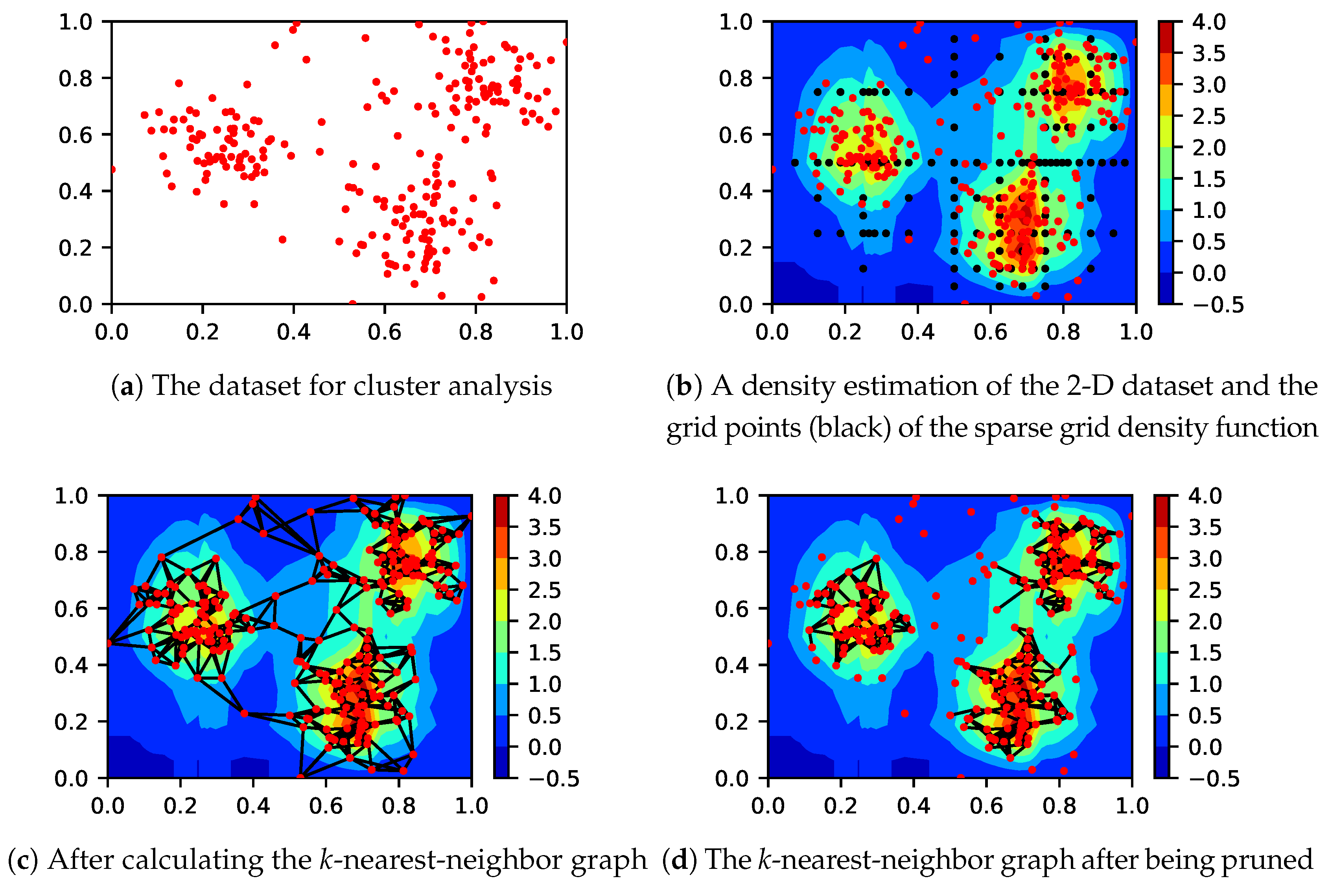
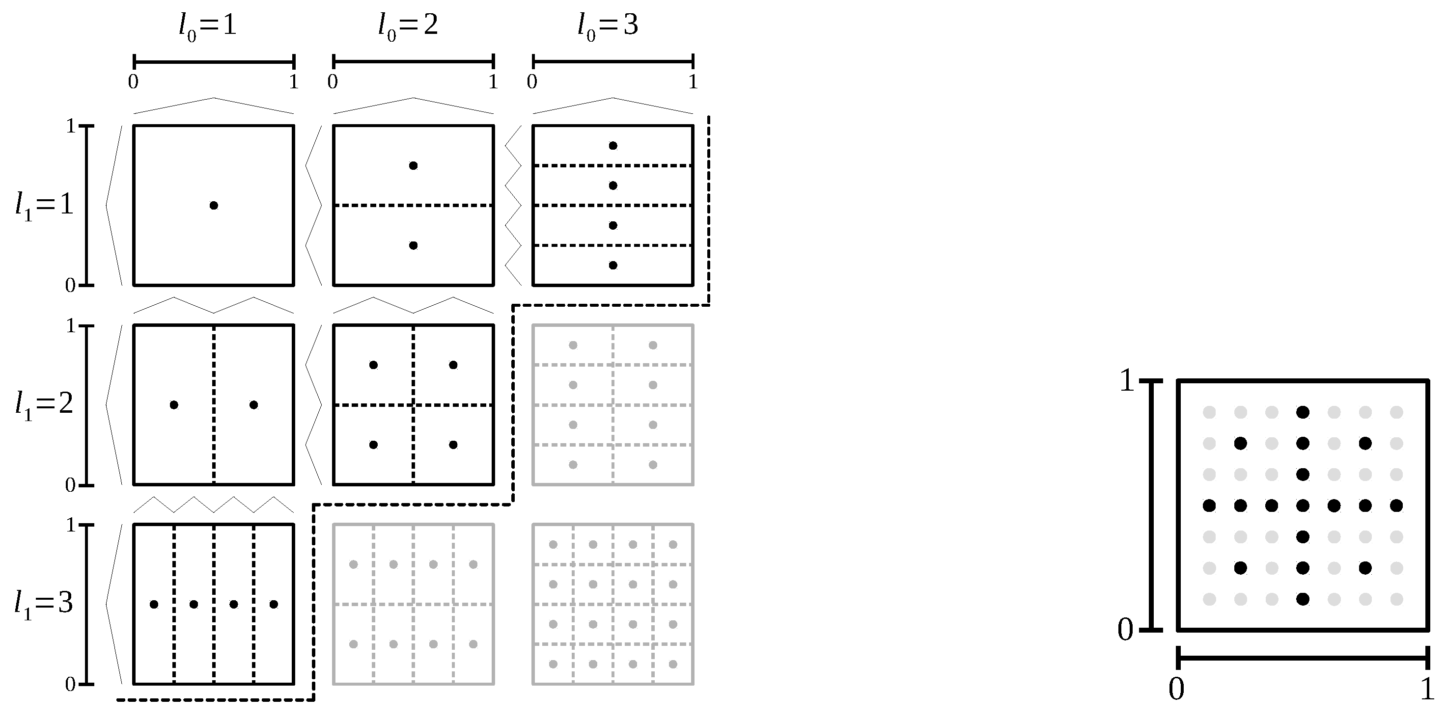
The sparse grid clustering algorithm is a four-step algorithm. Except for the last one, these steps are shown in Figure 1 using as an example a 2-D dataset with three clusters. The sparse grid clustering algorithm first calculates a density estimation of the dataset using the sparse grid density estimation algorithm (Figure 1b). Sparse grids use a set of grid points at which basis functions are centered; these are shown as black dots. As the next step, a k-nearest-neighbor graph of the dataset is computed (Figure 1c). In the third step, the density estimation is used to prune the graph. The algorithm prunes nodes in low-density regions and edges that intersect low-density regions (Figure 1d). In the fourth and final step the weakly connected components of the pruned graph are retrieved. The connected components of the graph are returned as the detected clusters.

This description suggests an important parameter of the algorithm. To decide whether to prune a node or edge from the k-nearest-neighbor graph, the sparse grid clustering method requires a density threshold value t. Nodes are pruned from the k-nearest-neighbor graph if the density at their location is below t. Edges are removed if they intersect regions with density values below t.

3. Estimating Densities on Sparse Grids

The sparse grid density estimation is built upon the concept of sparse grids. We therefore, introduce sparse grids and then describe how densities can be estimated with the sparse grid method.

3.1. Sparse Grids

As this work focuses on the sparse grid clustering algorithm and not on the basic sparse grid method, we only introduce the concepts required to understand the core algorithms of sparse grid clustering. For further information and in-depth explanations, we refer to the overview by Bungartz and Griebel [27] which follows the same notations. The core ideas include a spatial discretization of the (normalized) feature space, enabled by an incremental, adaptive, hierarchical formulation of underlying basis functions in one dimension. Its extension to arbitrary-dimensional settings can be truncated to keep the effort low.

A d-dimensional grid can be defined on the unit hypercube ${[0,1]}^d$ with an equidistant mesh width $h_n=2^{-n}$ for a discretization level $n\in \mathbb{N}$ and, therefore, 2nd grid points. With basis functions centered at the grid points, a corresponding function space is spanned by the linear combinations of the basis functions. We call this a full grid approach. Full grids can be represented in a hierarchical basis. From this representation, it is a small step to sparse grids.

The hierarchical approach constructs a final grid by superimposing a set of subgrids. First, we define an index set that is used to enumerate the grid points on the d-dimensional subgrids of discretization level $\mathbf{l}\in {\mathbb{N}}^d$:

$$I_{\mathbf{l}}:=\{(i_1,\cdots ,i_d):0<i_k<2^{l_k},i_k\mathrm{odd}\}.$$

(2)

In this work, we employ hat functions as basis functions. The scaled and translated 1-D hat functions are defined as

$${\varphi }_{l,i}\left(x\right):=max(0,1-|2^{l}x-i\left|\right).$$

(3)

For $d>1$, we use a tensor-product approach:

$${\varphi }_{\mathbf{l},\mathbf{i}}\left(\mathbf{x}\right):=\prod _{j=1}^d{\varphi }_{l_j,i_j}\left(x_j\right).$$

(4)

Given an index set $I_{\mathbf{l}}$ and the basis functions ${\varphi }_{\mathbf{l},\mathbf{i}}$, we can define the subspaces

$$W_{\mathbf{l}}:=\mathrm{span}\{{\varphi }_{\mathbf{l},\mathbf{i}}:\mathbf{i}\in I_{\mathbf{l}}\}.$$

(5)

The subgrids and their grid points $x_{\mathbf{l},\mathbf{i}}:=(i_1{h}_{l_1},\cdots ,i_d{h}_{l_d})$ for the subspaces $W_{(1,1)}\cdots W_{(3,3)}$ are displayed in Figure 2a for a 2-D grid.

With the direct sum ⨁, a full grid of discretization level $n\in \mathbb{N}$ in the hierarchical basis can be defined as

$$V_n:=\underset{{\left|\mathbf{l}\right|}_{\infty }\le n}{⨁}{W}_{\mathbf{l}}.$$

(6)

Figure 3 shows how a 1-D grid is represented in the standard (nodal) basis (Figure 3a) and the hierarchical basis (Figure 3b).

Sparse grids are based on the observation that for sufficiently smooth functions only a small additional interpolation error is introduced if certain grid points are removed [27]. This mitigates the issue of dimensionality. As a result, the sparse grid function space $V_n^{\left(1\right)}$ is constructed from a different set of subspaces:

$$V_n^{\left(1\right)}:=\underset{{\left|\mathbf{l}\right|}_1\le n+d-1}{⨁}{W}_{\mathbf{l}}.$$

(7)

Figure 2 shows how a 2-D sparse grid is constructed from subgrids that correspond to the subspaces of the grid.

A sparse grid function $f\in V_n^{\left(1\right)}$ is given as

$$f\left(\mathbf{x}\right)=\sum _{{\left|\mathbf{l}\right|}_1\le n+d-1}\sum _{\mathbf{i}\in I_{\mathbf{l}}}{\alpha }_{\mathbf{l},\mathbf{i}}{\varphi }_{\mathbf{l},\mathbf{i}}\left(\mathbf{x}\right)=\sum _{j=1}^N{\alpha }_j{\varphi }_j\left(\mathbf{x}\right),$$

(8)

where we sum up all N weighted basis functions in some order, and where N denotes the total number of grid points. Since our algorithms iterate the basis functions linearly, we use the simplified notation when the algorithms are presented. The coefficients ${\alpha }_{\mathbf{l},\mathbf{i}}$ are usually referred to as surpluses.

3.2. The Sparse Grid Density Estimation

The sparse grid density estimation, originally proposed by Hegland et al. [28], uses an initial density guess $f_{ϵ}$ than is smoothed using a spline-smoothing approach:

$$\widehat{f}=\underset{u\in V}{\arg \min }{\int }_{\Omega }{(u\left(\mathbf{x}\right)-f_{ϵ}\left(\mathbf{x}\right))}^2-D\mathbf{x}+{\lambda \left|\right|Lu\left|\right|}_{L_2}^2.$$

(9)

This approach results in a function $\widehat{f}\in V$ that balances closeness to the initial density guess with the regularization term ${\left|\right|Lu\left|\right|}_{L_2}^2$ that enforces smoothness on the resulting density function. The regularization parameter $\lambda$ controls the degree of smoothness of $\widehat{f}$. L usually is some differential operator. We use the initial density guess proposed by Hegland et al. that places a Dirac delta function ${\delta }_{{\mathbf{x}}_i}$ at every data point ${\mathbf{x}}_i$:

$$f_{ϵ}:=\frac{1}{m}\sum _{i=1}^m{\delta }_{{\mathbf{x}}_i}.$$

(10)

As in prior work, we compute the best sparse grid function $u\in V_n^{\left(1\right)}$ and use a surplus-based regularization approach [22]. Therefore, the problem to solve is

$$\widehat{f}=\underset{u\in V_n^{\left(1\right)}}{\arg \min }{\int }_{\Omega }{(u\left(\mathbf{x}\right)-f_{ϵ}\left(\mathbf{x}\right))}^2-D\mathbf{x}+\lambda \sum _{i=1}^N{\alpha }_i^2.$$

(11)

This formulation leads to a system of linear equations

$$\begin{array}{c}\hfill (B+\lambda I)\mathbf{\alpha }=\mathbf{b},\end{array}$$

(12)

with $B_{ij}={({\varphi }_i,{\varphi }_j)}_{L_2}$, the identity matrix I and $b_i=\frac{1}{m}{\sum }_{j=1}^m{\varphi }_i\left({\mathbf{x}}_j\right)$.

We solve this system of linear equations with a conjugate gradient solver (CG). Given this iterative solver, two major operations need to be performed: calculating the right-hand side once and computing the matrix-vector product ${\mathbf{v}}^{\prime }=(B+\lambda I)\mathbf{v}$ in every CG iteration. The calculation of the right-hand side is straightforward. However, the matrix-vector product requires efficient computations of the $L_2$ inner product of pairs of basis functions:

$$\begin{array}{cc}\hfill {({\varphi }_{\mathbf{l},\mathbf{i}},{\varphi }_{{\mathbf{l}}^{\prime },{\mathbf{i}}^{\prime }})}_{L_2}& ={\int }_{\Omega }{\varphi }_{\mathbf{l},\mathbf{i}}\left(\mathbf{x}\right){\varphi }_{{\mathbf{l}}^{\prime },{\mathbf{i}}^{\prime }}\left(\mathbf{x}\right)d\mathbf{x}\hfill \end{array}$$

(13)

$$\begin{array}{cc}\hfill & ={\int }_0^1{\varphi }_{l_1,i_1}\left(x_1\right){\varphi }_{l_1^{\prime },i_1^{\prime }}\left(x_1\right)d{x}_1\cdots {\int }_0^1{\varphi }_{l_d,i_d}\left(x_d\right){\varphi }_{l_d^{\prime },i_d^{\prime }}\left(x_d\right)d{x}_d.\hfill \end{array}$$

(14)

The 1-D integrals can be computed directly:

$${\int }_0^1{\varphi }_{l,i}\left(x\right){\varphi }_{l^{\prime },i^{\prime }}\left(x\right)dx=\left\{\begin{array}{cc}\frac{2}{3}{h}_l,\hfill & x_{li}=x_{l^{\prime }{i}^{\prime }},\hfill \\ h_{l^{\prime }}{\varphi }_{l,i}\left(x_{l^{\prime }{i}^{\prime }}\right)+h_l{\varphi }_{l^{\prime }{i}^{\prime }}\left(x_{li}\right),\hfill & \mathrm{else}.\hfill \end{array}\right.$$

(15)

We note that in many instances the integral will be zero due to the non-overlapping support of the hat functions.

Figure 4 shows the effect of varying the regularization parameter $\lambda$ for a 2-D dataset. $\lambda$ has to be chosen with care, as too small values might split a single cluster into multiple clusters. On the other hand, if $\lambda$ is too large separate clusters could be part of the same high-density region.

3.3. Streaming Algorithms for the Sparse Grid Density Estimation

A high-performance sparse grid density estimation algorithm needs to efficiently compute the two operations described above: the computations of the matrix-vector product ${\mathbf{v}}^{\prime }=(B+\lambda I)\mathbf{v}$ and the right-hand side $\mathbf{b}$ with $b_i=\frac{1}{m}{\sum }_{j=1}^m{\varphi }_i\left({\mathbf{x}}_j\right)$. To efficiently perform these operations, we use an implicit matrix approach. That is, components of the matrix B get re-computed whenever they are accessed. This approach might seem wasteful at first glance. However, as the size of B scales quadratically in the number of grid points, it quickly becomes infeasible to store the matrix in memory.

The computation of the right-hand side requires the computation of m vector components. Algorithm 1 shows the loop structure of a scalar version of this operation. As the basis function evaluations in the innermost loop are independent, we can parallelize this algorithm over the outer loop, i.e., the iteration over the grid points. The evaluation of hat functions is branch-free. Therefore, this algorithm is well-suited for vectorization.

Algorithm 1: The streaming algorithm for computing the right-hand side $\mathbf{b}$

We can formulate the matrix-vector operation as a second streaming algorithm with two nested loops over the grid points. This is shown in Algorithm 2. Similar to the hat function evaluations of the right-hand side, the $L_2$ norms can be independently computed as well. Thus, we can parallelize Algorithm 2 by processing the outer loop in parallel. The two cases for computing the 1-D integral according to Equation (15) slightly complicate vectorization. Our approach is the computation of both cases in a vectorized algorithm and a single conditional move to return the correct result. Computing the $x_{li}=x_{l^{\prime }{i}^{\prime }}$ case is only a single multiplication, as we can move the computation of $h_l=2^{-l}$ to a precomputation step. Therefore, and because the $x_{li}=x_{l^{\prime }{i}^{\prime }}$ case rarely occurs, the overhead in each integration step is low compared to an optimal algorithm that would only evaluate the correct integration case.

Algorithm 2: The streaming algorithm for computing the matrix-vector multiplication ${\mathbf{v}}^{\prime }=(B+\lambda I)\mathbf{v}$

4. Other Steps

In this section, we first present the algorithm for computing the k-nearest-neighbor graph. Then, we show how we apply the sparse grid density estimation to prune it. Finally, we describe how we perform the connected component search in the pruned graph.

4.1. Computing the k-Nearest-Neighbor Graph

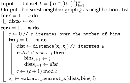
To create the k-nearest-neighbor graph, we have developed an approximate variant of the $\mathcal{O}\left((k+d)m^2\right)$ algorithm that compares all pairs of data points. Instead of creating a neighborhood list with k entries directly, we employ an approach with b bins that implicitly splits the dataset into b ranges. For every data point i the dataset is iterated. Thereafter, each bin contains the nearest neighbor of its assigned range of data points. To obtain an approximate k-nearest-neighbor solution, the k indices with the smallest associated distances are selected from the b bins. Pseudocode for this approach is displayed in Algorithm 3.

Algorithm 3: A variant of the $\mathcal{O}\left(m^2\right)$ k-nearest-neighbor algorithm that uses b bins.

This k-nearest-neighbor algorithm offers several advantages. It is not affected by the issue of dimensionality and therefore, works well for the higher-dimensional datasets we target. In contrast, spatial partitioning approaches such as k-d-trees tend to suffer from the issue of dimensionality. Furthermore, it maps well to modern hardware architectures as it is straightforward to parallelize and vectorize. Through cache blocking of the outer loop that iterates i, the resulting algorithm is highly cache-efficient as well. Finally, the number of neighbors k and the number of bins b are the only parameters to specify.

Binning was introduced for performance reasons. It allows us to only perform a single comparison in the innermost loop instead of k comparisons and, therefore, reduces the complexity to $\mathcal{O}\left(d{m}^2\right)$. The effect on the detected clusters is minimal, as it is very likely that nodes are still connected to close-by nodes of the same density region and therefore, the same cluster. Furthermore, edges that intersect low-density regions get pruned, as we describe in the next section.

The overall clustering algorithm is relatively robust with regard to different values of k. However, k should not be too small. Otherwise, the k-nearest-neighbor graph might be split into more connected components than are desired. For larger values of k, performance decreases slightly in the subsequent pruning step as the pruning algorithm has linear complexity in k. In our experience, choosing k with values between five and ten balances this trade-off. Consequently, we set b to 16, as it is larger than expected values of k and leads to a good-enough approximation of the k-nearest-neighbor graph. On modern hardware platforms, this choice of b should not increase the cache or register memory requirements of the algorithm to an extent that would affect performance.

4.2. Pruning the k-Nearest-Neighbor Graph

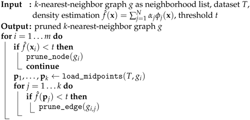
To prune the k-nearest-neighbor graph, we use two criteria. First, we remove data points and their corresponding edges in regions of low density. To this end, the density function is evaluated at the position ${\mathbf{x}}_i$ that corresponds to the current graph node $g_i$. The node and its edges are removed if the density is below a threshold t. Second, we remove edges that pass through regions of low density to separate nodes that belong to different clusters. As it is impossible to test all points along the corresponding line segment, we heuristically test only its midpoint, which has the largest distance to the two nodes belonging to high-density regions. If it falls below the threshold t, we remove the edge. Our pruning approach is shown in Algorithm 4.

Algorithm 4: A streaming algorithm for pruning low-density nodes and edges of the k-nearest-neighbor graph. The density function is evaluated at the location of the nodes and at the midpoints of the edges.

Similar to the other algorithms presented, iterations of the outer loop are independent and can therefore, be parallelized. The most expensive operations in this loop, multiple evaluations of the density function, are branch-free. Therefore, this algorithm is straightforward to vectorize as well. As there are only $\mathcal{O}(m·(k+1\left)\right)$ conditionals compared to overall $\mathcal{O}\left(m\right(k+1\left)N\right)$ operations, the conditionals do not significantly impact performance.

4.3. Connected Component Detection

To detect the weakly connected components in the pruned graph, we first convert the directed graph to an undirected graph by adding all inverted edges. Then, we perform a depth-first search to detect the connected components. This classical algorithm performs $\mathcal{O}\left(km\right)$ memory operations. Because the complexity of this algorithm is significantly lower compared to all other steps, this algorithm is only shared-memory parallelized and not distributed.

5. Implementation

In this section, we describe how our sparse grid clustering approach was implemented. To that end, we first consider the OpenCL-based node-level implementation and then present our distributed manager–worker approach.

5.1. Node-Level Implementation

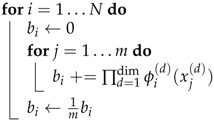
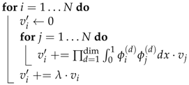
Except for the connected component detection, all steps of the clustering algorithm have been implemented as OpenCL kernels. There are two OpenCL kernels for the density estimation: one for calculating the right-hand side and one for the matrix-vector multiplication. A third OpenCL kernel implements the k-nearest-neighbor graph creation and a fourth kernel implements the density-based graph pruning.

From a performance engineering perspective, these OpenCL kernels have some commonalities. All kernels were parallelized over the outermost loop, exploiting the fact that the loop iterations are independent. Furthermore, all OpenCL kernels were designed to be branch-free with regard to their critical innermost loops. The only exception is the density matrix-vector multiplication kernel that has a single branch in the innermost loop. This branch is implemented using the OpenCL select function to differentiate between the integration cases. On modern OpenCL platforms, this should be compiled to a conditional move. Because only standard arithmetic is used and because of the regular control flow, the four computed kernels get vectorized on all OpenCL platforms we tested. Due to the design of the computed kernels, we expect this to be the case on many untested OpenCL platforms as well.

The local memory is used in all kernels to either share grid points or data points between all threads of the work-group. For example, the prune graph kernel evaluates 1-D sparse grid basis functions in its innermost loop. The threads of a work-group process different data points, but all always evaluate their data point with the same basis function. Therefore, the data of the currently processed basis function can be shared efficiently through the local memory. Furthermore, the data point assigned to a thread remains constant throughout the lifetime of the thread. It can therefore be stored in private memory, which translates to the register file on GPU devices and the L1 cache (or the registers) on processors.

Table 1. The number of floating-point operations for the different OpenCL kernels and the arithmetic intensities (in floating point operations per byte) for a work-group size (ws) of one thread and 128 threads. The peak limit states the achievable fraction of the peak performance given the instruction mix of the computed kernels.

Kernel	FP Ops./Complexity	Arith. Int. (ws = 1)	Arith. Int. (ws = 128)	Peak Lim. (%)
density right-hand side	$N·m·d·6$	$1.5$ FB−1	$192$ FB−1	67%
density matrix-vector	$\text{CG-iter}.·N^2·d·14$	$1.2$ FB−1	$149$ FB−1	64%
create graph	$m^2·d·3$	$1.0$ FB−1	$129$ FB−1	83%
prune graph	$m·N·(k+1)·d·6$	$4.5$ FB−1	$576$ FB−1	67%

shows the number of floating-point operations for the different OpenCL kernels. As both the number of grid points N and the size of the dataset m can be large, all operations are potentially expensive. In most data mining scenarios, the sparse grid will have significantly fewer grid points than there are data points. Therefore, the k-nearest-neighbor graph creation is expected to be the most expensive operation. Depending on the number of CG iterations, the density matrix-vector product can be moderately expensive as well. However, it only depends on the grid points and therefore, benefits from $N<m$.

To estimate the achievable performance of our computed kernels, we calculated the arithmetic intensities of our computed kernels. As Table 1 shows, the arithmetic intensities of a work-group with a single thread would be too low to achieve a significant fraction of the peak performance on modern hardware platforms (see

Table 2. The hardware platforms used in the distributed and node-level experiments. We list the frequency type that best matches our observations during the experiments.

Device	Type	Cores/Shaders	Frequency	Peak (SP)	Mem. Bandw.	Machine Balance
Tesla P100	GPU	3584	$1.3$$\mathrm{G}$$\mathrm{Hz}$ (boost)	$9.5$$\mathrm{T}$$\mathrm{F}$	720 GB s−1	$12.9$ FB−1
FirePro W8100	GPU	2560	$0.8$$\mathrm{G}$$\mathrm{Hz}$ (max)	$4.2$$\mathrm{T}$$\mathrm{F}$	320 GB s−1	$13.2$ FB−1
2xXeon E5-2680v3	CPU	24	$2.5$$\mathrm{G}$$\mathrm{Hz}$ (base)	$1.9$$\mathrm{T}$$\mathrm{F}$	137 GB s−1	$14.0$ FB−1

for the machine balances of the hardware platforms we used). However, with a larger work-group size of 128 threads, and because we efficiently use the shared memory, the arithmetic intensity is strongly improved. On processor-based platforms, the L1 cache enables similarly high arithmetic intensity values. As a consequence, the performance of our computed kernels on all platforms is only bound by ALU performance and memory bandwidth is not a concern.

The arithmetic intensity values would allow our computed kernels to achieve peak performance. However, as our computed kernels make use of instructions other than fused-multiply add (FMA) operations, the instruction mix reduces the achievable performance. To calculate the peak limit given in Table 1, we make the (realistic) assumption that the remaining vector floating-point instructions run at half the performance of the FMA instructions [29].

5.2. Distributed Implementation

For distributed computing, we developed a manager–worker model that was implemented with MPI. To create work that can be assigned to the workers, we split the loops that were used for parallelization (the outermost loops of the computed kernels) once again. We use a static load balancing scheme that distributes the work equally to the workers. Our implementation supports single as well as double precision. Currently, we transfer double precision data even if single precision is used in the computed kernels.

From the perspective of the manager node, the distributed algorithm consists of four major steps: creating the right-hand side of the density estimation, the density matrix-vector products, an integrated graph-creation-and-prune step and the connected component search. These steps are shown in Figure 5. Note that the matrix-vector multiplication step (Figure 5d) is repeated once per CG iteration.

When the application is started, the dataset is read by the manager node and sent to all workers, requiring $m·d·8$ bytes of communication per worker. Then, the manager node creates the grid and sends it to the workers as well. This requires $2·N·d·8$ bytes per worker to be communicated. After these relatively expensive transfers are completed, grid and dataset are held by the workers. Therefore, most remaining communication steps only require small amounts of data to be transferred. We demonstrate in Section 6 that the overhead of these communication steps is indeed very low compared to the computational requirements of the remainder of the algorithm. To read the dataset, we use the standard C++ API. Advanced techniques to improve I/O performance, such as MPI I/O, are currently not used.

To compute the density right-hand-side operation, every worker computes an index range of the components of $\mathbf{b}$. As $\mathbf{b}$ is aggregated on the manager node, $N·8$ bytes need to be transferred. During each CG step and after the final CG step, the manager sends $\mathbf{v}$ ($\mathit{\alpha }$ after the final iteration) to all workers. Each worker calculates the result of an index range of ${\mathbf{v}}^{\prime }$ and communicates the partial result back to the manager node. Therefore, $N·8$ bytes per worker are communicated during each iteration and after the final iteration. Collecting the partial results for ${\mathbf{v}}^{\prime }$ requires another $N·8$ bytes to be transferred per CG step.

The creation of the k-nearest-neighbor graph only requires the assignment of index ranges and no further communication. Because the pruning of the k-nearest-neighbor graph reuses the same index ranges that were assigned in the graph creation step, this step only requires the pruned graph to be sent to the manager node. This step requires $k·m·8$ bytes to be transferred. Having received the pruned graph, the manager node performs the connected component detection and has thereby computed the clusters.

6. Results

In this section, we evaluate our distributed and performance-portable sparse grid clustering approach. We first present the hardware platforms and datasets that were used in the experiments. Then we provide the results of our node-level experiments that demonstrate performance portability. The quality of the clustering is discussed in the context of the node-level experiments as well. Finally, we present distributed performance results for two supercomputers: Hazel Hen and Piz Daint.

6.1. Hardware Platforms

On the node level, we used three different hardware platforms. Two of them are GPUs: the Nvidia Tesla P100 and the AMD FirePro W8100. To represent standard processor platforms, we used a dual socket machine with two Intel Xeon E5-2680v3 processors. The relevant technical details of these hardware platforms are summarized in Table 2.

Our distributed experiments were conducted on two supercomputers. The Cray XC40 Hazel Hen is an Intel processor-based machine with 7712 nodes for a peak performance of $7.4\mathrm{P}\mathrm{F}$. Hazel Hen is located at the High Performance Computing Center Stuttgart (HLRS) in Stuttgart, Germany. It has dual socket nodes with Xeon E5-2680v3 processors and $128\mathrm{G}$ of memory per node.

The Cray XC40/XC50 Piz Daint is a mostly GPU-based supercomputer with a peak performance of $27\mathrm{P}\mathrm{F}$. Piz Daint is located at the Swiss National Supercomputing Centre (CSCS) in Lugano, Switzerland. Each of the XC50 nodes that we used have a single Intel Xeon E5-2690v3 processor with $64\mathrm{G}$ of memory and a single Nvidia Tesla P100 GPU. In our experiments, we only used the Tesla P100 to compute the main computed kernels of our application.

6.2. Datasets and Experimental Setup

In all of our experiments, we used synthetic datasets with clusters drawn from Gaussian distributions with randomly drawn means ${\mu }_i$ and equal standard deviation $\sigma$. The ${\mu }_i$ thus are the cluster centers. We normalized the datasets to ${[0.1,0.9]}^d$. As this moves data points sufficiently towards the center of the domain, we can use a sparse grid without boundary grid points.

The parameters used to generate the datasets are listed in

Table 3. The Gaussian datasets for the distributed and the node-level runs.

Name	Size	Clust.	$\mathit{\sigma }$	Dim.	Dist.	Noise	Type
10M-3C	10M	3	0.12	10	$3·\sigma$	0%	distributed
100M-3C	100M	3	0.12	10	$3·\sigma$	0%	distributed
1M-10C	1M	10	0.05	10	$7·\sigma$	2%	node-level
1M-100C	1M	100	0.05	10	$7·\sigma$	2%	node-level
10M-100C	10M	100	0.05	10	$7·\sigma$	2%	node-level

. The datasets with 100 clusters are challenging, as the density estimation needs to correctly separate 100 high-density regions in a setting of moderately high dimensionality. Furthermore, to make it possible to assess the quality of the clustering, we generated the node-level dataset so that the clusters are well-separated by forcing a minimum distance of $7·\sigma$ between the cluster centers. We verified that the noise connects all clusters in the unpruned k-nearest-neighbor graph.

We use synthetic datasets for several reasons. First, clustering problems have no general well-defined solution [10]. To estimate the performance of our approach, we need access to the “ground truth” of the underlying class labels. For real-world datasets this is typically missing or has been reconstructed by manual and error-prone labeling. Here, we use the adjusted Rand index (ARI) to measure the quality, which requires a reference clustering. Second, we want to ensure that the data set is challenging for our approach. The clusters’ densities are ensured to be of maximum dimensionality. In particular, their dimensionality cannot be reduced in contrast to many real-world datasets. Furthermore, they form the worst case for the sparse grid density estimation [22]. Finally, competitive clustering performance for real-world datasets has already been shown for smaller datasets without distributed computing in previous work [21].

The experiments depend on a set of parameters which are shown in

Table 4. The parameters used for configuring the clustering algorithm and the adjusted Rand index (ARI) for the node-level experiments. In the distributed runs, the threshold was specified as a fraction of the maximum surplus of the density function. The node-level runs used an absolute threshold value.

Name	λ	Threshold t	Level	Grid Points	CG $\mathit{ϵ}$	k	ARI	Type
1M-10C	1E-5	667	6	76k	1E-2	6	1.0	node-level
1M-100C	1E-6	556	7	0.4M	1E-2	6	0.85	node-level
10M-10C	1E-5	1167	7	0.4M	1E-2	6	1.0	node-level
10M-100C	1E-6	1000	7	0.4M	1E-2	6	0.90	node-level
10M-3C	1E-6	$0.7·max\left(\mathit{\alpha }\right)$	7	0.4M	1E-3	5	-	distributed
100M-3C	1E-6	$0.7·max\left(\mathit{\alpha }\right)$	8	1.9M	1E-3	5	-	distributed

. The ARI is a quality measure for clustering and is addressed in Section 6.4. In all of our experiments, we used single-precision floating-point arithmetic.

6.3. Node-Level Performance and Performance-Portability

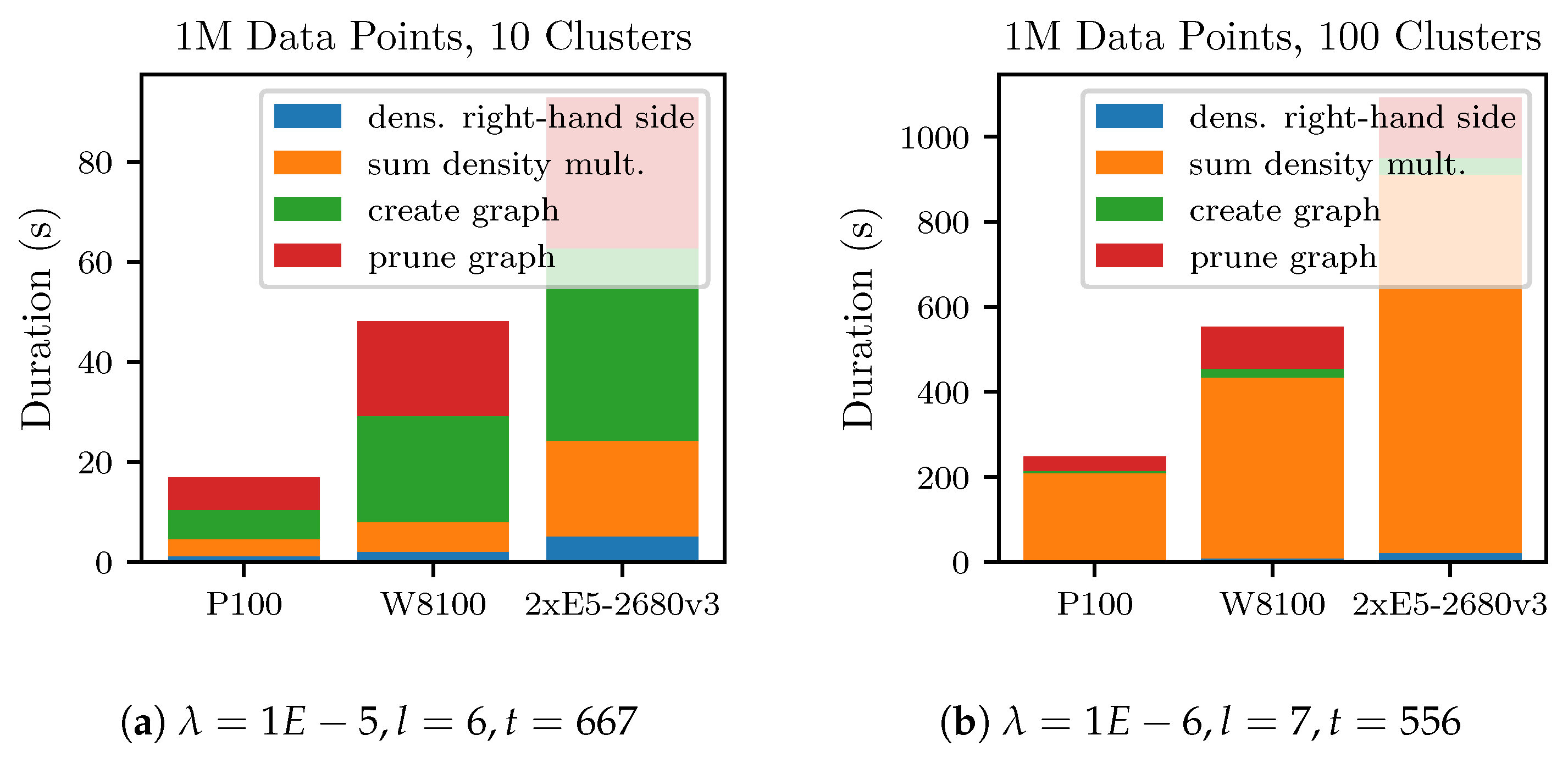
The Figure 6 and Figure 7 show the runtimes of the node-level experiments. For more consistent results, the runs were repeated four times and the measurements averaged. The 1M-10C dataset could be processed on a Tesla P100 in less than $20\mathrm{s}$. Processing the 1M-100C dataset is more time-consuming and required $248\mathrm{s}$ again using a Tesla P100. The main reason for the time increase is because the density estimation requires more time due to a larger sparse grid and a smaller $\lambda$, which leads to more CG iterations.

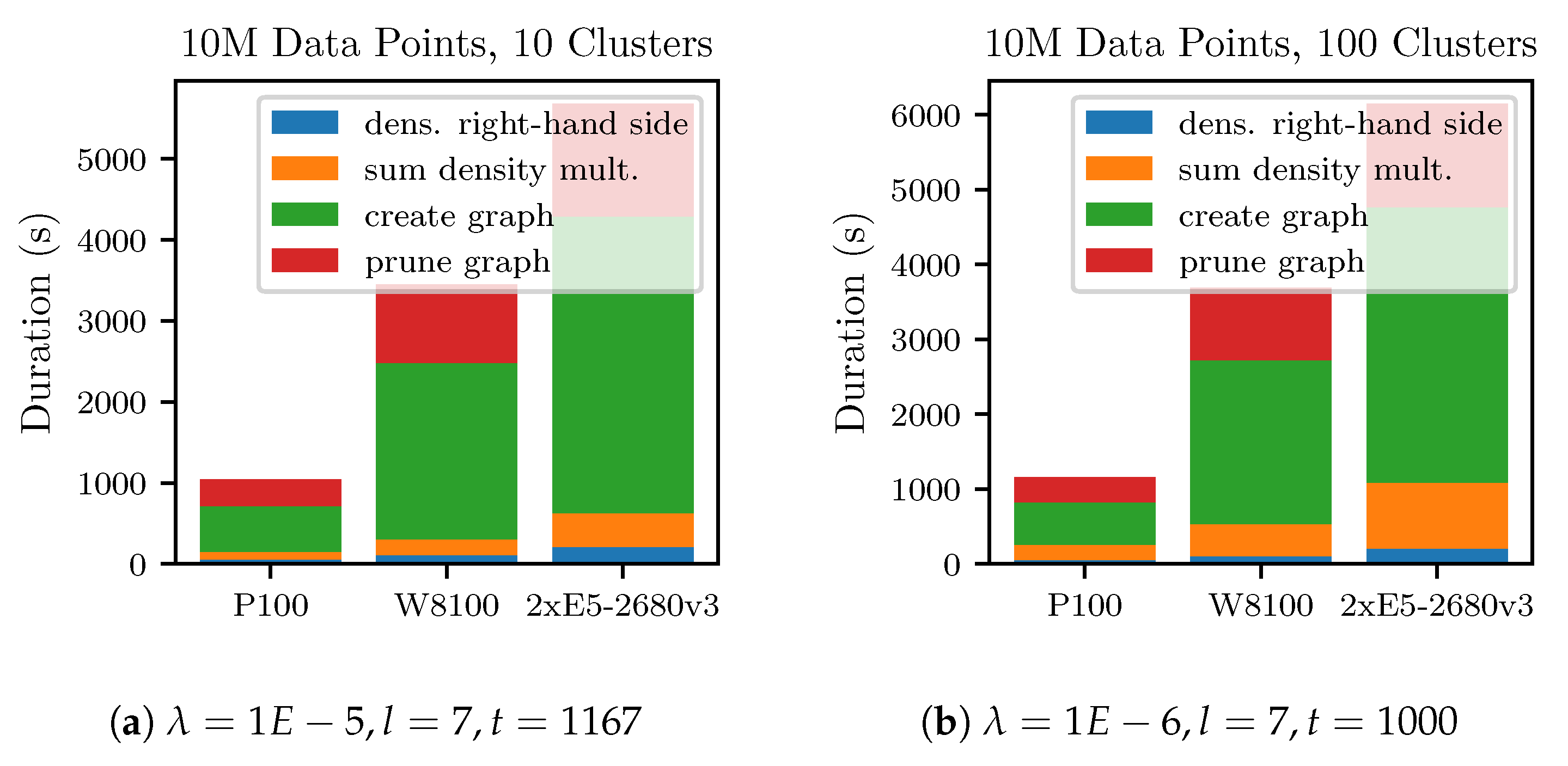
The experiments with the 10 million data points datasets are shown in Figure 7. Due to the increased size of the datasets, the k-nearest-neighbor graph creation takes up the largest fraction of the runtime in both experiments. This illustrates that for large datasets, because of its quadratic complexity, the k-nearest-neighbor graph creation step will dominate the overall runtime. In these two experiments, increasing the number of clusters has only a small effect on the runtime. Mainly, because in both cases a sparse grid with level $l=7$ was used. On the P100 platform, the experiments with the 10M-100C dataset took $1162\mathrm{s}$. The other hardware platforms took longer, proportional to their lower raw performance.

Table 5. The node-level performance of the clustering algorithm. All results are for single-precision arithmetic. The performance was measured with the 10M-10C dataset and the parameters listed in Table 4. Note that the achievable peak performance is limited by the instruction mix to values significantly below 100%.

Kernel	Result Type	Tesla P100	FirePro W8100	2xE5-2680v3
dens. right-hand side	GFLOPS	4584	2271 ($753\mathrm{M}\mathrm{Hz}$)	1177
limit: 67% peak	peak (of lim.)	48% (72%)	59% (88%)	61% (91%)
dens. matrix-vector	GFLOPS	4090	1939 ($759\mathrm{M}\mathrm{Hz}$)	919
limit: 64% peak	peak (of lim.)	43% (67%)	50% (78%)	48% (75%)
create graph	GFLOPS	5474	1433 ($467\mathrm{M}\mathrm{Hz}$)	852
limit: 83% peak	peak (of lim.)	58% (70%)	60% (72%)	44% (53%)
prune graph	GFLOPS	5360	1817 ($822\mathrm{M}\mathrm{Hz}$)	1265
limit: 67% peak	peak (of lim.)	56% (84%)	43% (64%)	66% (99%)

shows the performance achieved in the node-level experiments. It displays the performance in GFLOPS and the achieved fraction of peak performance. The achieved fraction of the peak performance relative to the instruction-mix-based limit is displayed as well. These results were calculated from the runs with the 10M-10C dataset as specified in Table 4.

Our implementation achieved a significant fraction of the peak performance across all devices. Additionally, if the limit imposed by the instruction mix is taken into account, we see that many combinations of kernels and devices run close to their maximally achievable performance. The only kernel that reaches less than two-thirds of its achievable performance is the create graph kernel on the Xeon E5 platform. We suspect that this is due to throttling of the processor, as this operation puts extreme stress on the vector units.

The fastest device by a significant margin is the Tesla P100, as it is the most recent of the devices and has the highest theoretical peak performance. It is $2.23-3.29$x faster than the W8100 and $4.41-5.49$x faster than the Xeon E5 pair.

The FirePro W8100 achieves similar fractions of the peak performance compared to the P100 at a lower absolute level of performance. It is still $1.67-1.98$x faster than the pair of Xeon E5 processors. During our experiments, the FirePro W8100 displayed strong throttling which is why we list the average frequencies observed for the invidivual computed kernels. The reduced frequencies imply lower achievable peak performance ($2·2560·f_{\mathrm{avr}}$) which we take into account for the calculation of the peak performance and the resulting achieved fraction of peak performance. The average frequencies reported were measured in a separate run of the 10M-10C experiment. In case of the k-nearest-neighbor graph kernel, a frequency of only $492\mathrm{M}\mathrm{Hz}$ was measured. This nearly halves the achievable performance of this computed kernel.

Because it has the lowest absolute performance, the pair of Xeon E5 processors scores lowest. However, the achieved fractions of the peak performance are similar to the other devices. This indicates that performance is not only portable across GPU platforms, but processor-based platforms as well.

6.4. Clustering Quality and Parameter Tuning

This work mostly focuses on the performance of our sparse grid clustering approach. Nevertheless, to make our evaluation more realistic, we tuned the clustering parameters of our node-level runs for (nearly) optimal clustering quality. For a more detailed discussion of the achievable level of quality, we refer to prior work which compared sparse grid clustering to other clustering algorithms [21]. A comparison of the sparse grid density estimation to other density estimation methods is available as well [30].

To assess the quality, we used the adjusted Rand index (ARI) which compares two cluster mappings. Because we know the mapping of data points to clusters of each of our synthetic datasets, these reference cluster mappings were compared to the output of the sparse grid clustering algorithm. The calculated ARI of the node-level experiments is shown in Table 4. These results show that we can nearly perfectly reconstruct the clusters of both datasets with ten clusters. The datasets with 100 clusters are more challenging and would require slightly larger grids for further improvements.

Even though we know the clusters we want to detect, we still need to find parameter values for the sparse grid clustering algorithm that lead to the desired cluster mapping. Some parameters can be chosen conservatively and then adjusted manually for a higher quality clustering or improved performance. As an initial guess for the sparse grid discretization level, it can be chosen so that the size of the grid is equal to a fraction of the dataset. k and $ϵ$ can be conservatively chosen with 10 and ${10}^{-6}$, respectively. However, $\lambda$ and t depend on each other and have no obvious default values. We therefore, employ a parameter tuning approach to find values for these two parameters.

During parameter tuning, we first select a value for the regularization parameter $\lambda$ and then search for the best pruning threshold t. For each value of $\lambda$ and t, we make use of the available reference clustering and compute the ARI which we maximize. As search strategies, we implemented an approach with two nested binary searches. The overall best parameter combination encountered is returned as the result.

The ARI requires a reference solution which, of course, it not available for yet unsolved problems. However, this basic parameter tuning approach can be applied more generally if an application-dependent quality metric is provided to assess a computed clustering. Note that in contrast to other data mining tasks such as regression, there is no well-defined solution independent of the application context. Therefore, this is not a limitation of the sparse grid clustering approach.

To speed up parameter tuning, our sparse grid clustering implementation allows for reusing of the k-nearest-neighbor graph and calculated density estimations. As the k-nearest-neighbor graph is the same independent of all parameters, it can be calculated once overall. Moreover, the density estimation changes only if $\lambda$ is changed. Thus, the density estimation can be reused while an optimal value for t is searched. Only the comparably cheap graph pruning operation and the connected component search are performed at every parameter tuning step.

6.5. Distributed Results on Hazel Hen

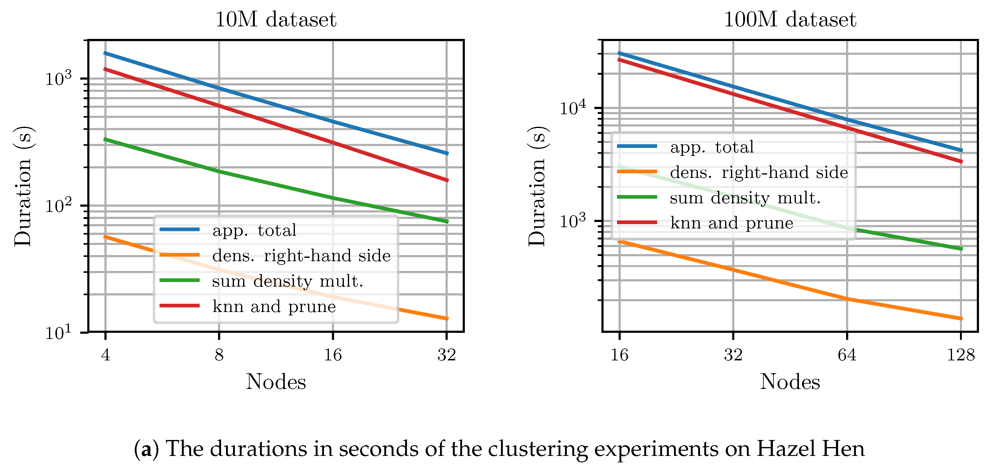
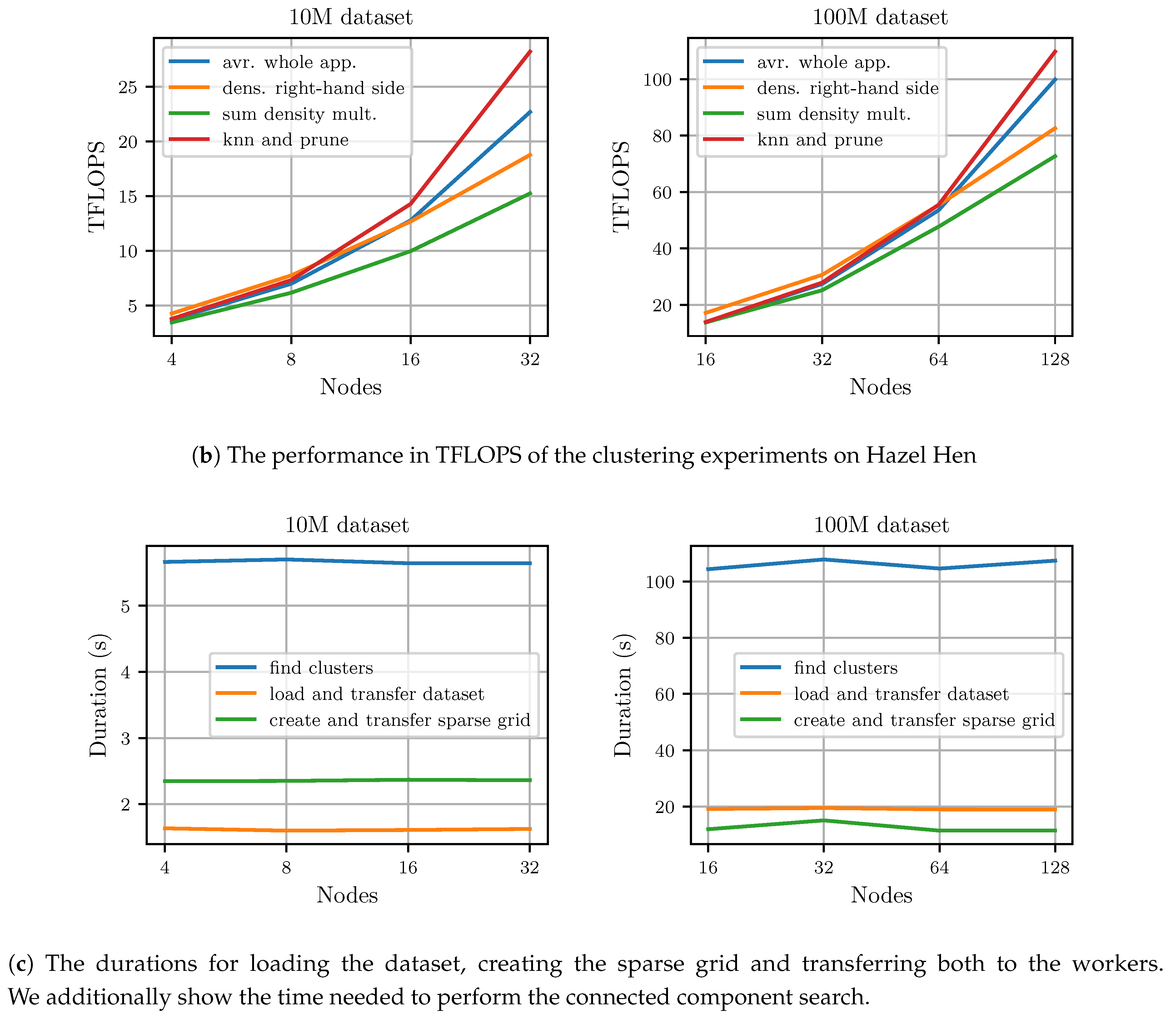
Figure 8 shows the results of the distributed experiments conducted on Hazel Hen. Results are given for the individual computed kernels as well as the whole application run. The total runtime, and the average application TFLOPS derived from it, is based on the wall-clock time of the application and not only on the three major distributed operations. At the highest node count, it took $4226\mathrm{s}$ to process the 100M-3C dataset and $259\mathrm{s}$ to process the 10M-3C dataset. We achieved up to $100\mathrm{TFLOPS}$ for the 100M-3C dataset using 128 nodes and up to $23\mathrm{TFLOPS}$ for the 10M-3C using 32 nodes. Therefore, we achieved 41% and 37% of the peak performance at the highest number of nodes for the whole application including all communication and file input–output operations.

The creation and pruning of the k-nearest-neighbor graph scales nearly linearly. Calculating the density estimation scales slightly worse. As the grid is much smaller than the dataset, there is too little work available per node during the density estimation step to achieve optimal performance at high node counts.

Figure 8c displays the duration of the initial loading and distribution of the dataset, the creation and the transfer of the sparse grid and the duration of the connected component search. As Figure 8c shows, loading and communicating the dataset does not take up significant amounts of time. The same is true for creating and transferring the sparse grid. However, the connected component search becomes relatively expensive for the 100M-3C dataset, as it is performed on a single node and therefore, cannot scale with an increasing number of nodes. Nevertheless, at 128 nodes the connected component search still only requires $107\mathrm{s}$ or $2.5$% of the total runtime for the 100M-3C dataset. For the 10M-3C dataset and 32 nodes, the connected component search takes up $2.2$% of the total runtime.

6.6. Distributed Results on Piz Daint

We conducted the distributed experiments before we were able to do some final node-level optimizations, and due to compute time limitations we were not able to recompute the experiments. Thus, the results of these experiments are not directly comparable to the node-level performance results. Since these experiments, the node-level performance of all computed kernels was improved. Because of this, scalability might by slightly overestimated. Furthermore, the duration of the connected component search is not listed in these results, as we used a different algorithm at the time of the experiments.

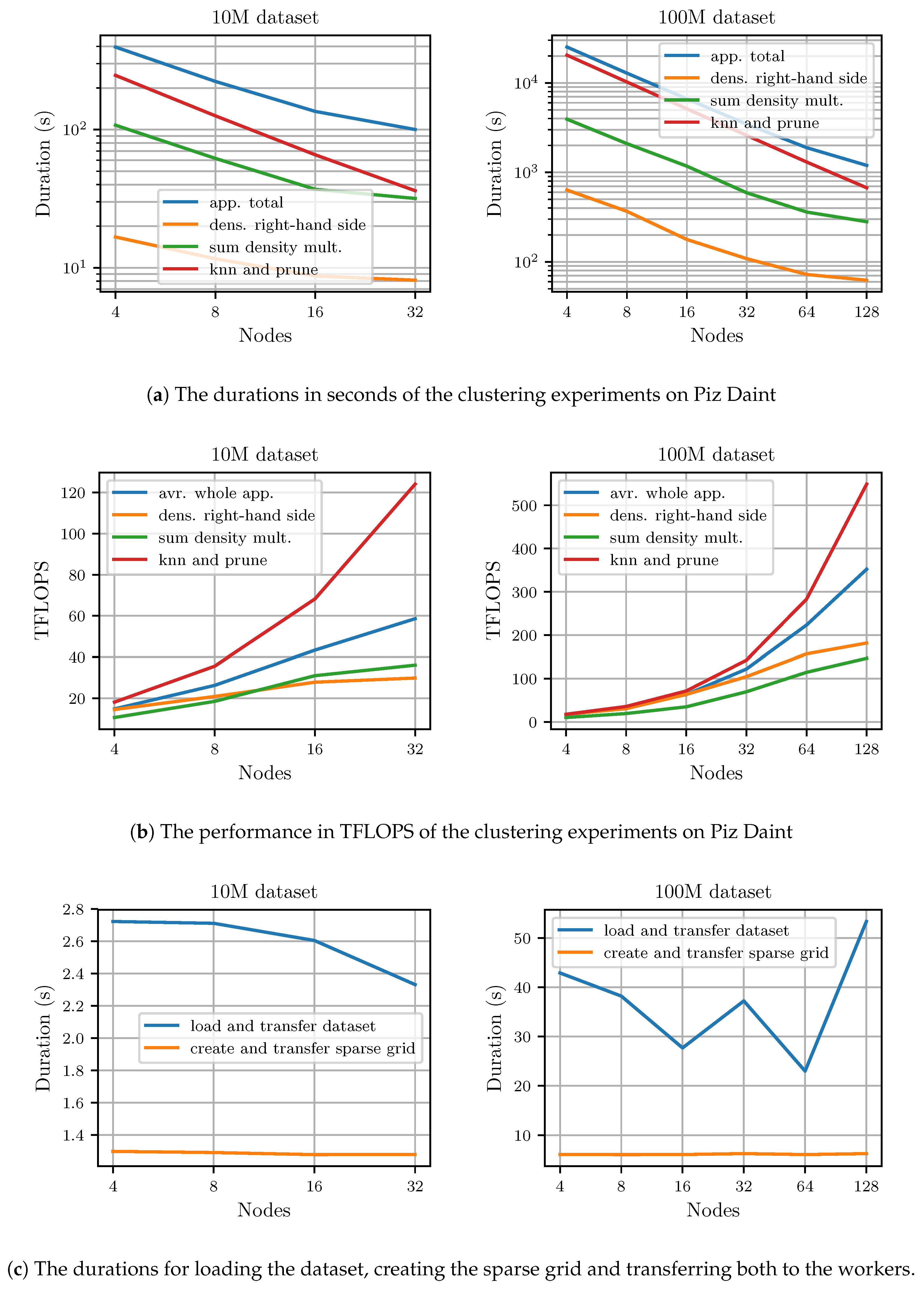
Figure 9 shows duration and performance of the experiments performed on Piz Daint for both the 10M-3C and 100M-3C datasets. Again, results are given for the individual computed kernels as well as the whole application run. As Figure 9a shows, the application scales well to 128 nodes. Similar to the Hazel Hen results, the integrated graph-creation-and-prune step scales nearly linearly, whereas the density estimation scales slightly worse. Using 32 nodes, the clustering of the 10M-3C dataset takes $100\mathrm{s}$. It takes $1198\mathrm{s}$ to cluster the 100M-3C dataset using 128 nodes. This translates to an average performance of $59\mathrm{TFLOPS}$ for the 10M-3C dataset and $352\mathrm{TFLOPS}$ for the 100M-3C dataset as Figure 9b shows. Thus, at 128 nodes our implementation still achieves 29% of the peak performance for the whole application including all communication and the loading of the dataset.

Figure 9c displays the duration of the initial loading and distribution of the dataset and the creation and transfer of the sparse grid to the workers. Only the loading of the dataset is somewhat expensive.

Compared to Hazel Hen, the performance on Piz Daint is consistently higher, which is explained by the difference in node-level performance. However, due to the processor-based architecture, Hazel Hen nodes require less work per node to be fully utilized. Therefore, on Hazel Hen a slightly higher fraction of peak performance was achieved.

7. Discussion and Future Work

Sparse grid clustering, as implemented in the open source library SG${}^{++}$, is one the few clustering methods available for the clustering of large datasets on HPC machines. In contrast to other density estimation approaches, our approach based on sparse grids does not depend on assumptions about the underlying densities and which can treat correlated densities [30,31]. In particular, it enables the detection of clusters with non-convex shapes and without a predetermined number of clusters; see [21] for the comparison to other clustering algorithms. Due to the sparse grid discretization of the underlying feature space, the grid or discretization points are chosen independently of the data points. This is key to the linear complexity with respect size of the data of all sparse-grid-related algorithms. This rare property is highly useful for addressing big data challenges. Note that there is little work on distributed clustering on large scale for big data scenarios, see the discussion in Section 1.

With our optimized implementation, we have demonstrated performance portability across three hardware platforms. Due to the use of OpenCL, careful and highly tuned performance optimization, and algorithms that map very well to the capabilities of modern hardware platforms, we expect similar performance on related platforms. Our strong scaling experiments show that even on 128 nodes of Piz Daint, scalability is mainly limited by the available work per node.

Our method achieves a significant fraction of the peak performance on all devices tested. This shows that OpenCL is a good choice for developing performance-portable software. Furthermore, our GPU results illustrate how the higher raw performance of GPUs in contrast to CPUs translates to similarly improved time-to-solution.

As our next steps, we plan to further improve the performance of our approach by addressing two key issues: First, the k-nearest-neighbor graph creation currently uses an $\mathcal{O}\left(m^2\right)$ algorithm and thus represents the bottle-neck. We already have an early implementation of a GPU-enabled variant of the locality-sensitive hashing algorithm. The locality-sensitive hashing algorithm can calculate an approximate k-nearest-neighbor graph in sub-quadratic complexity [32]. Adopting this algorithm, sparse grid clustering can be performed in sub-quadratic complexity as well.

Our implementation supports the use of spatially adaptive sparse grids [22,30]. They enable the placement of grid points only where they significantly contribute to the overall solution. An adaptive approach will significantly increase the dimensionality of the datasets that can be clustered as it has been demonstrated for standard learning tasks before. Currently, creating an adaptively refined sparse grid is itself expensive as it requires the system of linear equations of the density estimation to be solved repeatedly after each refinement. Thus, a priori refinement strategies that create well-adapted sparse grids with less effort are another important direction of future research.

8. Materials and Methods

The source code of this study will be made available as part of the sparse grid toolbox SG${}^{++}$ at the time of publication [33]. We archive the scripts for creating the synthetic datasets at the same location.