1. Introduction
Several metaheuristic algorithms have now been developed inspired by nature [
1]. Some have been inspired by fireflies [
2], birds [
3], bats [
4], buffaloes [
5,
6], flowers [
7], corals [
8] or even the harmony of a song [
9]. These metaheuristics have helped shorten resolution times for problems in the mining, transportation, planning, and other areas. The areas where we can apply metaheuristics also cover topics that pertain to artificial intelligence [
10]. Among the topics, there are different types of life simulations. One type of simulation is to design a dynamic prey–predator spatial model to observe the behavior of prey and predators in real time [
11,
12,
13,
14]. Preys and predators can be designed using cellular automata.
The cellular automata are moving in a theoretical world formed by a lattice that has the form of a torus. The movement of predators can be modeled using the equations of motion of the metaheuristics. This integration is possible because there is a conceptual relationship in moving within a search space for metaheuristics or moving within a lattice for cellular automata. In this research, we focused on applying the movement of African buffalo optimization (ABO) metaheuristics [
5,
6] in the movement of predator migration. In addition, an agent-based architecture is proposed for the control of the population of prey and predator.
Multi-Agent Systems (MAS) can help adapt various behaviors in real time. For example, they can help adjust the population in real time in prey–predator simulations. However, other aspects must be considered to perform a prey–predator simulation. Among them, we have the cellular automata [
15,
16], which allow modeling prey and predators easily. In addition, to construct the virtual world in which the cellular automatons move, one must consider using a lattice. In this lattice, the cellular automata can increase and decrease its population. In addition, it is possible to keep a record of the population and of the different states that have the cellular automata.
The rest of this article is structured as follows: In
Section 2, we discuss the related work, including the major motivations for performing this research. In
Section 3, the theory of cellular automata is revised.
Section 4 explains the African buffalo optimization metaheuristic.
Section 5 describes how to implement the prey–predator dynamics model using the ABO metaheuristic algorithm equations incorporating a population control using multi-agents.
Section 6 explains the experiments and discussion. Finally,
Section 7 concludes and provides guidelines for future work.
2. Background
The related work is organized as follows: First, research using cellular automata is reviewed. Then, we examine the different versions that have been developed for the prey–predator model. Subsequently, investigations applying cellular automata and agent systems in prey–predator models are reviewed. Finally, we describe the motivation of this article and the benefits of this research.
2.1. Prey–Predator
Different versions of prey–predator models have been applied to various areas or problems. In [
17], a prey adaptation as a cause of predator–prey cycles. This research analyzes a simple model of prey–predators with an adaptive change in a feature of the prey. This change determines the speed at which prey is captured by predators. A set of equations that describe the dynamics of the population of many species interacting in food webs is applied in [
18]. Pang and Wang [
19] reviewed a strategy and stationary pattern in a three-species predator–prey model. Wang [
20] focused on a reaction–diffusion system that emerges from a prey–predator model of three species with predatory and reason-dependent functional responses, in which they studied the global existence and the bifurcation of non-permanent positive stationary states.
Other studies have focused on investigating the adaptive dynamics of prey–predator systems [
21]. These have been modeled with a dynamic system, in which the traits of prey and predators have allowed them to evolve through small mutations. In some approaches, they authors tried to understand a stochastic eco-evolutionary model of a prey–predator community [
22], i.e., they tried to understand the phenotypic coevolution of prey and predators.Finally, a review has examined recent theories on the evolution of prey–predator interactions [
23]. These theories cover topics on dynamics and stability in populations regarding their features on predicting how the traits of predators and anti-predators must respond to environmental changes.
2.2. Cellular Automata
In the area of cellular automata [
15,
24], different types of investigations have been carried out. Batty et al. [
25] reviewed the modeling of urban dynamics through cellular automata based on Geographic Information System (GIS). Cellular automata and fractal urban form are applied to a cellular modeling approach to the evolution of urban land-use patterns [
26]. A stochastic cellular automata solution is found to the density classification problem [
27]. An outer–inner fuzzy cellular automata algorithm is used for the dynamic uncertainty multi-project scheduling problem [
28]. Duplicated image regions are detected using cellular automata [
29]. The efficiency of cellular automata is improved for sewer network design optimization problems using adaptive refinement [
30]. An unconventional complex system is modeled via cellular automata and differential evolution [
31]. Finally, several articles reviewing the area of cellular automata have been published [
32,
33,
34,
35].
Cellular Automata with Prey–Predator
Automata network predator–prey model with pursuit and evasion is studied in [
36]. Spatial aspects of inter-specific competition are studied in [
37]. The effects of cell size and configuration in cellular automaton based prey–predator modeling are studied in [
38]. The threshold of coexistence and critical behavior of a predator–prey cellular automaton is studied in [
39]. A predator–prey cellular automaton with parasitic interactions and environmental effects is studied in [
40]. Dynamic prey–predator model simulations as a theoretical population of prey and living predators are studied in [
11]. Modeling of prey–predator dynamics via particle swarm optimization and cellular automata is studied in [
11]. Prey–predator dynamics and swarm intelligence on a cellular automata model are studied in [
12]. The spatial dynamics and oscillatory behavior of a predator–prey model based on cellular automata and local particle swarm optimization are studied in [
13]. The spatial dynamics of a prey–predator lattice model with social behavior are studied in [
14].
2.3. Agent System
A multi-agent system is a group of two or more agents working together to develop a particular task. These systems have the ability to communicate with each other to make decisions and thus perform a task in a simpler way. Multi-Agent systems are currently used in different applications, ranging from e-commerce [
41,
42,
43] to education [
44,
45,
46].
Agent System Applied to Prey–Predator Model
Mathieu et al. [
47] reviewed environment updating and agent scheduling policies in agent-based simulators that examine the purpose of observing the sensitivity of the parameters in the implementations of simulators based on agents. They considered upgrading the environment and agent scheduling policies. A distribution based on the environment and the other on the agents is studied in [
48]. This research has shown that some types of applications are more suitable for one type of distribution than others. In the experiments, using flocking and prey–predator models is considered. A stochastic scheme to model an artificial prey–predator ecosystem of several species to study the influence of energy flow on the useful life and stability of the ecosystem is investigated in [
49]. In [
50], the authors applied a computer model based on ecosystem agents to predict the interactions of competition and predation. Cyclic competition and percolation in grouping predator–prey populations is reviewed in [
51]. It shows that the properties of the Lett–Auger–Gaillard spatial model when different strategies coexist. These can be understood through the geometric behavior of clusters involving four effective strategies that compete cyclically, without neutral states.
2.4. Purpose of the Investigation
Several approaches have been made using metaheuristics [
11,
12,
13,
14,
52] in the resolution of the dynamic prey–predator spatial model, but none has integrated African buffalo optimization metaheuristics with the use of multi-agents to control population. The objective of this research was to propose the following approaches.
Model the motion of cellular automata using the motion equations of the African buffalo optimization metaheuristic [
5,
6,
53,
54,
55,
56,
57,
58,
59].
Use a multi-agent system for the development of the dynamic prey–predator spatial model, to maintain a balance of prey and predators in its environment.
For the dynamic prey–predator spatial model, perform five experiments for each type of approach, with and without multi-agents.
These contributions have not been reported yet.
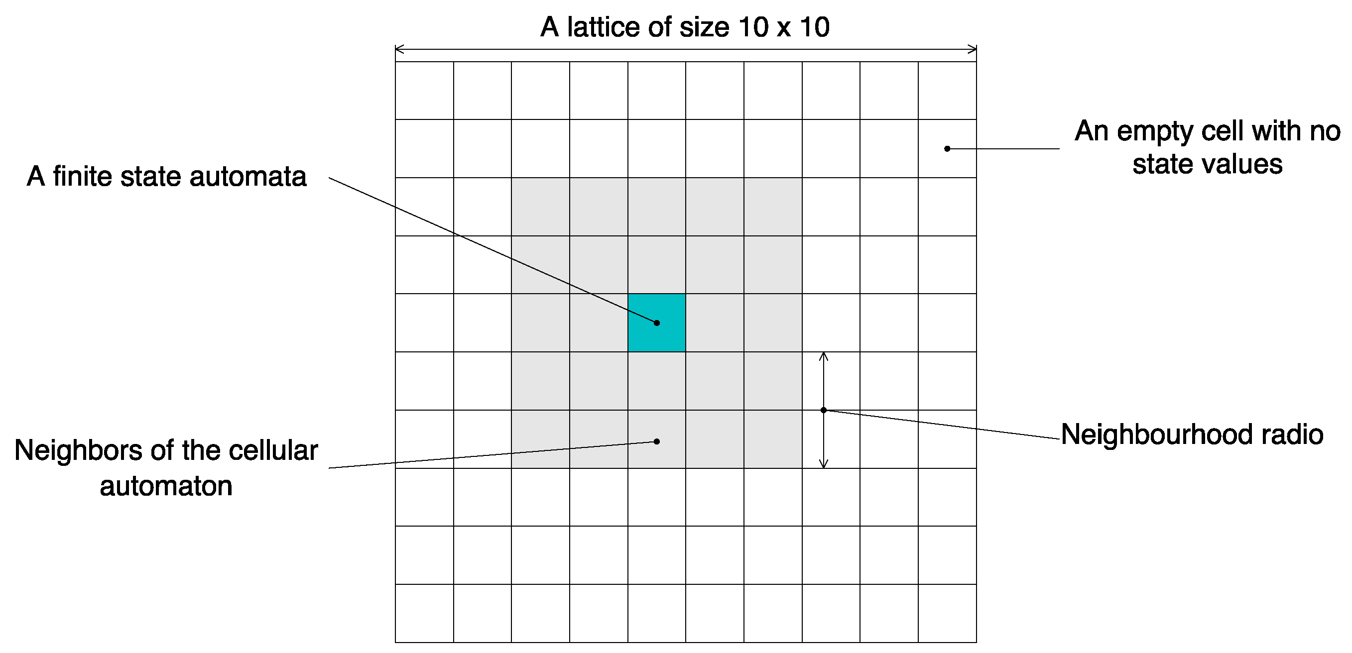
3. Cellular Automata
A Cellular Automaton (CA) is a kind of model system of cellular objects that have the following characteristics:
Cells live on a grid of a finite number of dimensions n. Generally, the grid is called a lattice.
Each cell in the lattice has a state. The number of state possibilities is typically finite. For example, a cell can have two or three options: 1 and 0; a, b, or c; or prey or predator.
Each cell in the lattice has a neighborhood. The neighborhood can be defined in different forms, but it is typically a list of adjacent cells.
4. African Buffalo Optimization
African buffalo optimization is a stochastic metaheuristic algorithm, which belongs to the branch of population algorithms [
5]. The ABO metaheuristic is inspired by the behavior of the African buffalo when they perform the migration of the herd. The migration of buffaloes aims to find better land for grazing. For this, they tend to follow the movement of the rainy seasons. To find good herbs the buffalo can be organized through two basic modes of communication:
The warning sound “waaa” indicates the presence of hazards or lack of good grazing fields. It also enables buffaloes to be able to explore other places that may be beneficial to the herd.
The “maaa” warning sound is used to indicate that a grazing area has a benefit for the herd. It is also an indication that animals continue to take advantage of available resources.
African Buffalo Optimization Algorithm
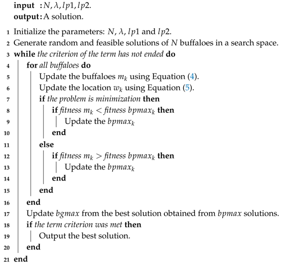
The ABO steps are detailed in Algorithm 1.
| Algorithm 1: African buffalo optimization algorithm. |
![Algorithms 12 00059 i001]() |
The parameters used on Line 1 of the algorithm are described below.
A number of N buffaloes, in which each buffalo m will represent a solution.
The Index k for the buffaloes, with k in .
The lambda value with a domain in , excluding the zero.
The learning factors and with a real number domain in .
On Line 5, Equation (
4) is used. The
variable represents the exploitation move. The
variable is the herd’s best fitness. The
variable is the individual buffalo
k best found location. Finally, the
variable represent the exploration move.
On Line 6, Equation (
5) represents when the location of buffalo
k is updated.
5. Dynamic Prey–Predator Spatial Model via African Buffalo Optimization
The dynamic prey–predator spatial model simulates a theoretical population of prey and predators. For the model designed by Martínez-Molina et al. [
11] and adapted in this research, the following concepts are defined.
5.1. Lattice Definition
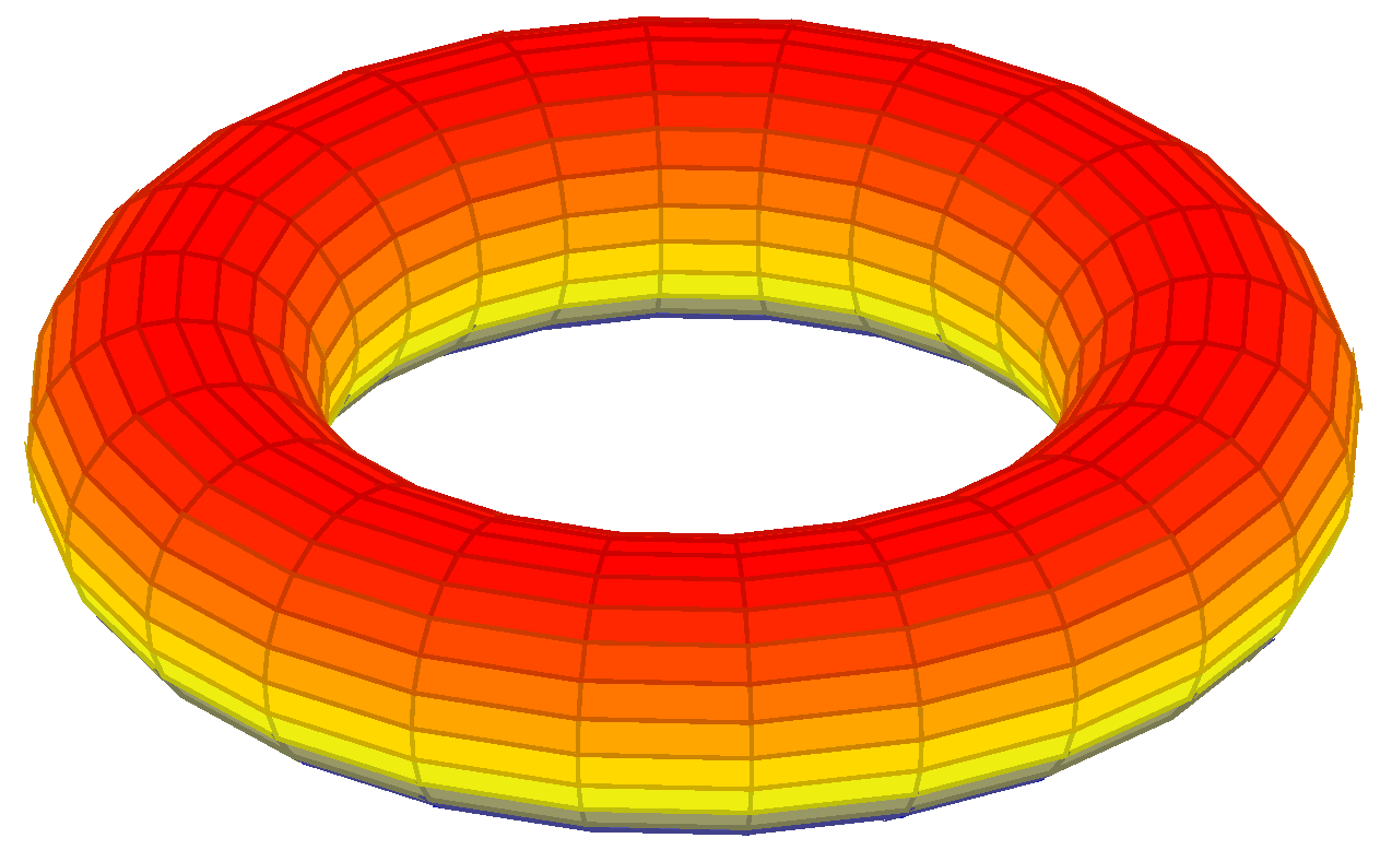
The lattice
L used has the shape of a torus (see
Figure 2).
A torus can be defined parametrically by:
where
,
are angles that make a full circle, thus their values start and end at the same point;
R is the distance from the center of the tube to the center of the torus;
r is the radius of the tube;
R is known as the major radius; and
r is known as the minor radius. The ratio
R divided by
r is known as the aspect ratio.
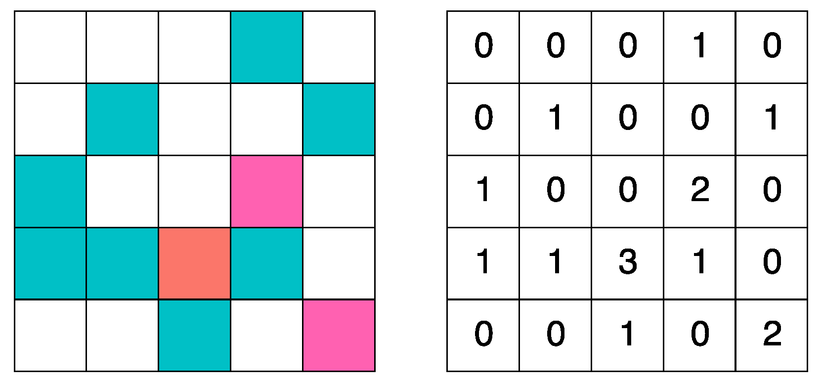
The values of allowed states for each cell is , where: 0 is an empty cell, 1 is a cell inhabited by a prey, 2 is a cell inhabited by a predator, and 3 is a cell that containing a prey and a predator at the same.
Figure 3 shows a visual representation of the values of the lattice.
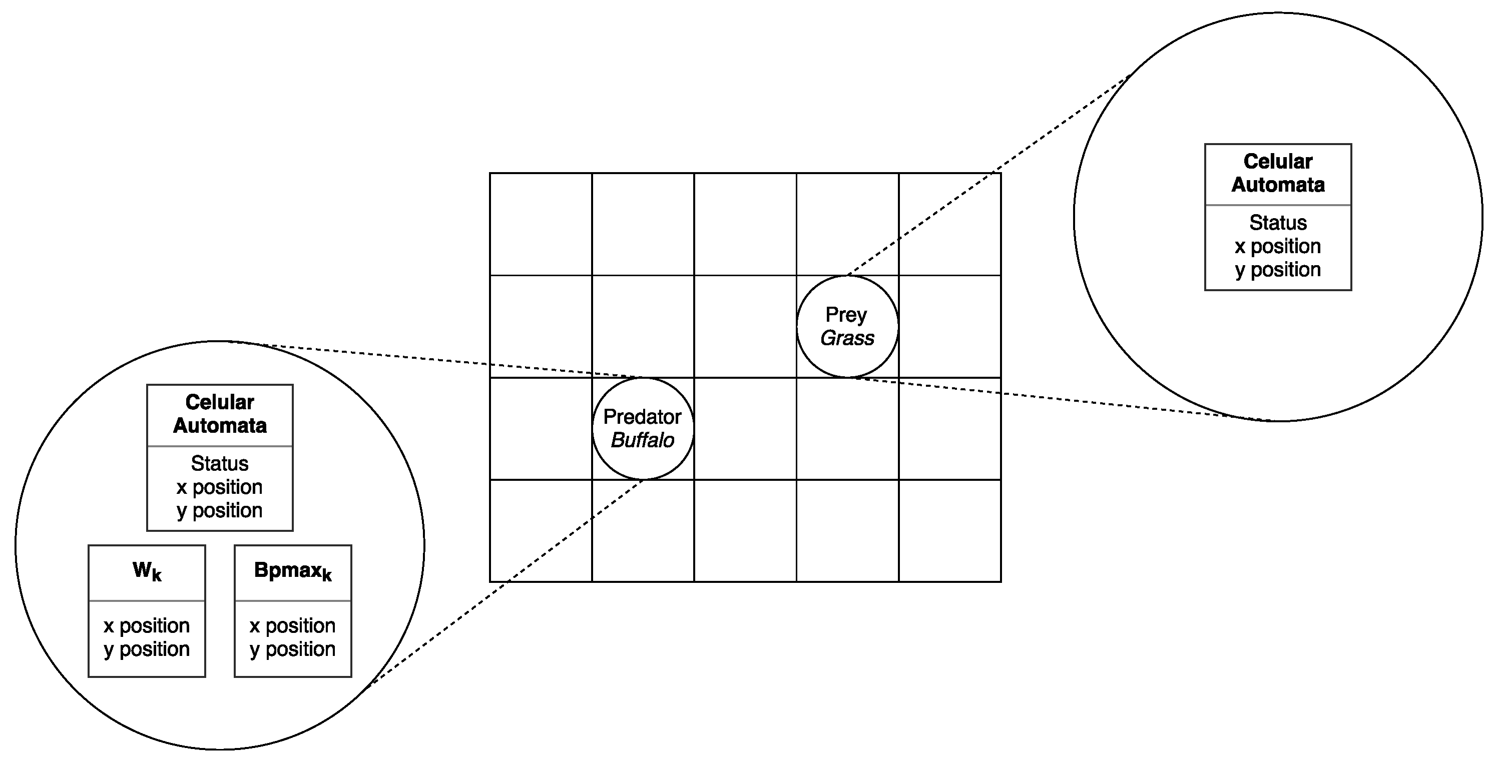
5.2. Cellular Automata Definition
There are two types of cellular automata: predators (
buffaloes) and prey (
grasslands). Predators are those who use the behavior of ABO metaheuristic. They have been designed in such a way to support an extra group of variables (see
Figure 4, left). Prey are those that use the behavior determined by the prey–predator dynamic model rules (see
Figure 4, right).
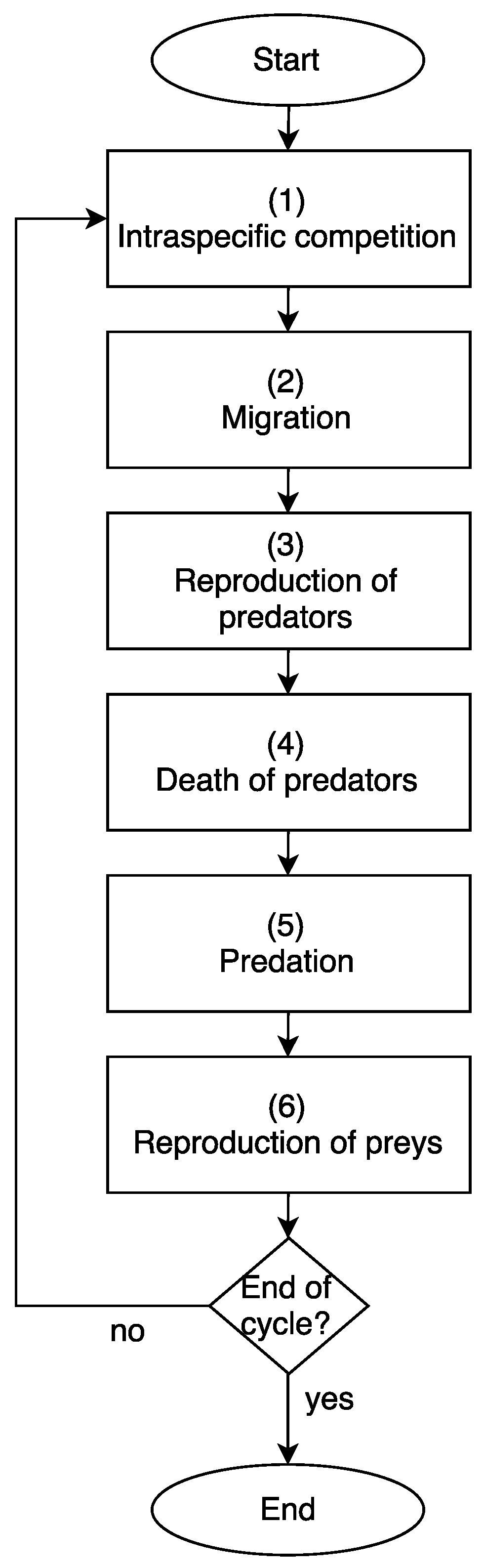
5.3. Season Definition
The model is composed of a life cycle that has the following stages or seasons (see
Figure 5).
Table 1 summarizes the main abbreviations with their meanings that have the various equations and procedures of prey and predators.
The description of each component in
Figure 5 is detailed below.
5.3.1. Intraspecific Competition
Preys die with a probability proportional to the number of individuals of the prey species surrounding them. This rule uses
neighborhood. In the lattice, if
, the probability of death
p is given by Equation (
7) [
14], where
is the intraspecific competence factor,
is the number of prey in the neighborhood, and
is the number of neighbor calculated by Equation (
8). The description of this procedure is detailed in Algorithms 2 and 3.
| Algorithm 2: Intraspecific competition. |
![Algorithms 12 00059 i002]() |
| Algorithm 3: Calculate . |
![Algorithms 12 00059 i003]() |
5.3.2. Migration
At this stage, the predators (
buffaloes) move within the space of the lattice according to the individual experience of each buffalo and the experience of the herd. To perform the migration of each predator, the new position (x, y) is calculated according to Equations (
9)–(
12). The description of this procedure is detailed in Algorithm 4.
| Algorithm 4: Migration. |
![Algorithms 12 00059 i004]() |
5.4. Reproduction of Predators
At this stage, predators breed by creating new individuals at random within the neighborhood by Equation (
13). The description of this procedure is detailed in Algorithm 5.
| Algorithm 5: Reproduction of predators. |
![Algorithms 12 00059 i005]() |
5.4.1. Death of Predators
Predators that do not have a prey in their own cell die from starvation (cellular automata with status equal to 2). The description of this procedure is detailed in Algorithm 6.
| Algorithm 6: Death of predators. |
![Algorithms 12 00059 i006]() |
5.4.2. Predation
All the prey that share a cell with a predator die due to the action of the predator (cellular automata with state equal to 3). The description of this procedure is detailed in Algorithm 7.
| Algorithm 7: Predation. |
![Algorithms 12 00059 i007]() |
5.4.3. Reproduction of Preys
Each prey creates new individuals randomly within the neighborhood. The description of this procedure is detailed in Algorithm 8.
| Algorithm 8: Reproduction of prey. |
![Algorithms 12 00059 i008]() |
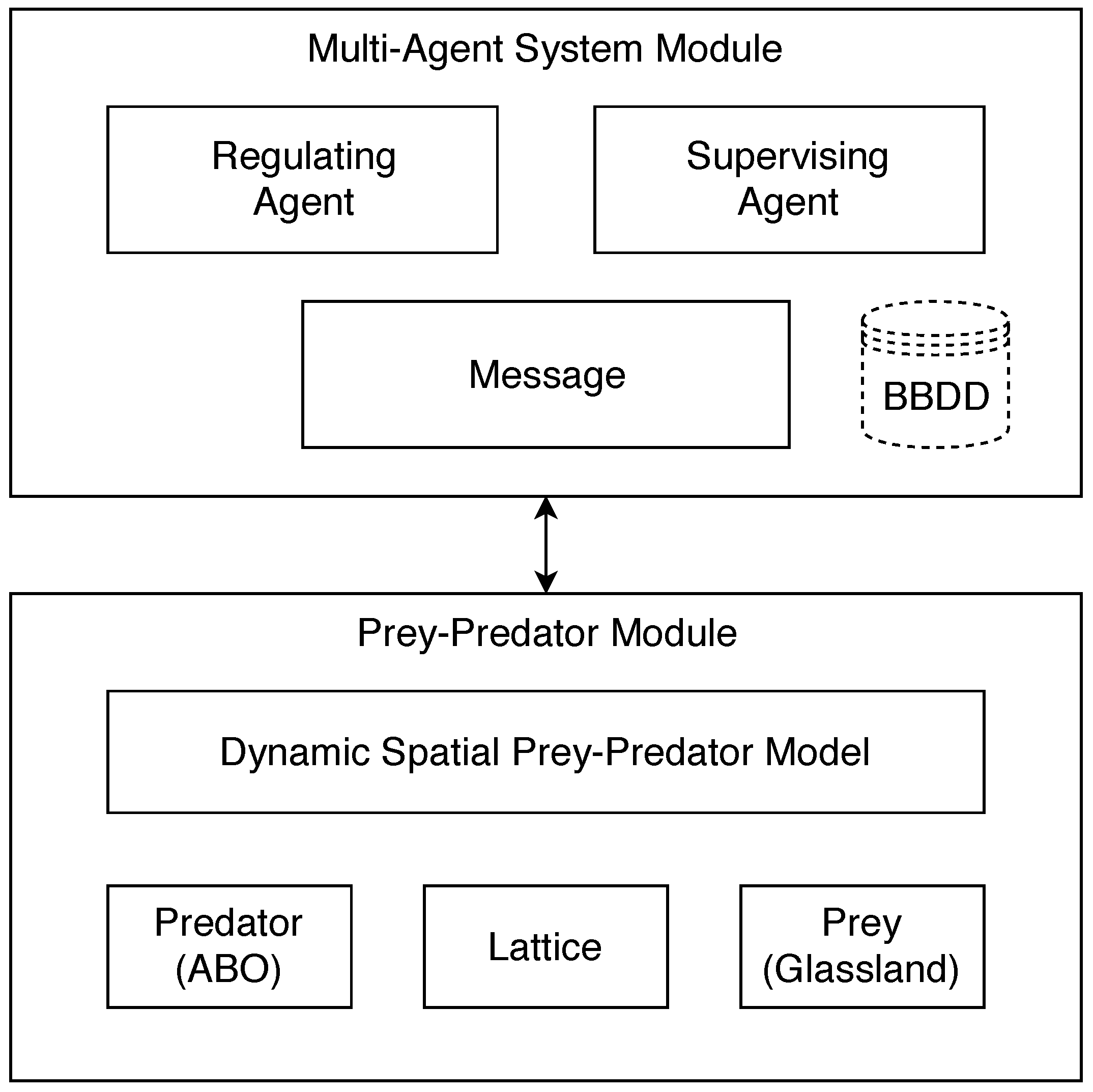
5.5. Multi-Agent System
The dynamic prey–predator spatial model can extend its characteristics using multi-agents. Using multi-agents, we can easily regulate the population of predators in an
online context (at runtime).
Figure 6 describes the main components of the architecture used in the design of the dynamic prey–predator spatial model.
The main modules for the agent system are described below.
5.5.1. Supervising Agent
This agent aims to capture the data of the prey–predator model as the iterations of the simulation progress. Subsequently, the supervising agent sends a message to the regulating agent. When the regulating agent has already responded to the message to the supervising agent, it automatically stores the data in a database (text BBDD with the number of prey, the number of predators and states of the lattice). These data are used by the next cycle of the prey–predator model. Once the data sent by the regulatory agent are stored, the supervising agent makes a call to a submodule in which the cycles of the model are controlled. This submodule is in charge of recharging the prey–predator model again using the parameters stored in the database. The idea is to create a balance and continuity in the model so that it can prevent a predator eats prey.
5.5.2. Regulating Agent
The regulating agent is initialized and is automatically waiting to receive a message form supervising agent. The regulating agent at the moment of receiving a message reacts and automatically performs calculations to verify the new parameters that should receive the model and thus generate a balance. The parameter that the regulating agent modifies is the capacity of reproduction. This parameter directly influences the prey–predator model, generating a balance between prey and predator. After generating and sending the data to the supervising agent, the regulating agent is automatically waiting for a new message to make new modifications respective.
The multi-agent approach modifies in real time the reproductive capacity of prey and predators using Equations (
15) and (
16), where
A is the number of prey in the lattice,
is a positive value assigned to regulate the prey population,
B is the number of predators in the lattice, and
is a positive value assigned to regulate the predator population.
5.5.3. Prey–Predator Module
This module includes basic features such as the dynamic prey–predator spatial model, the logic of the predator with the integration of the movements of the ABO metaheuristic, the prey logic, and the lattice constraints.
6. Experiments and Discussion
This section details the experiment performed and the observations found. Two types of approaches were performed, one using multi-agents to regulate the population and the other without using agents. Each method included five types of experiments, which varied depending on the parameters of the African buffalo optimization metaheuristics.
For the dynamic prey–predator spatial model configuration, the experimental parameters using for the model are described in
Table 2. The parameters of the prey were chosen in such a way that, at the beginning of the execution of the model, there was theoretically many prey, with a large radius of reproduction and competition. The parameters of the predator were such that there were initially few predators, with a small radius of reproduction.
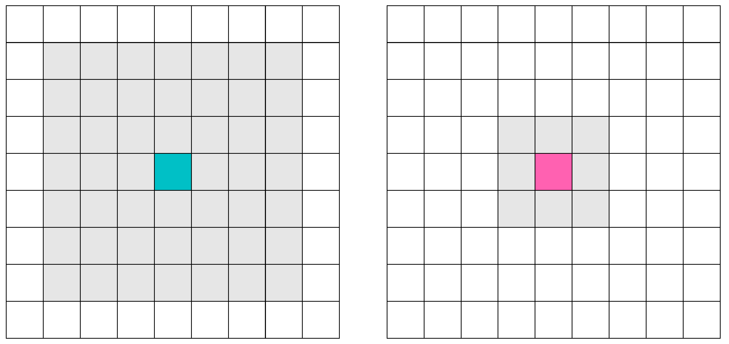
The rules for the Moore Neighborhood are visualized in
Figure 7. A lattice of 50 by 50 was used, giving a total of 2500 cells.
The experimental parameters used for the ABO metaheuristic are described in
Table 3. The idea was to have different parameter configurations for ABO metaheuristics.
For the multi-agent approach, the reproductive capacity of prey and predators using Equations (
15) and (
16) were modified in real time, with
of 800 and
of 6.
For the implementation, all simulation were coded in Java version 1.8.0_92 using IntelliJ IDEA 15 (15.0.6). For running the Dynamics Prey–Predator Spatial model, we used Java(TM) SE Runtime Environment (build 1.8.0_92). The hardware used was a MacBook Pro computer (Retina, 13-inch, Late 2013), with an Intel Core i5 2,4 GHz, 4 GB RAM 1600 MHz DDR3, running the OSx El Capitan version 10.11.6 (15G1004).
Results
Table 4,
Table 5,
Table 6,
Table 7 and
Table 8 show the results obtained without using agents.
Table 9,
Table 10,
Table 11,
Table 12 and
Table 13 show the results obtained using agents. All tables show only the first season and the last season. The description of the columns of the tables is described as follows: Column ID is the identifier for each row; Column ID-S is the identifier for each season; Column ID-SS is the identifier for each step in the season; Column Name-SS corresponds to the name of each step of the simulation; Column ID-M corresponds to the identifier for the migration (the simulation has five migrations); and Columns N-Prey and N-Predator show the number of prey and predator in the lattice, respectively.
For the parameters
and
equal to 1, the number of final prey was 80 and the number of predators was 1332 (see
Table 4).
For the parameters
and
equal to 2, the number of final prey was 93 and the number of predators was 1322 (see
Table 5).
For the parameters
and
equal to 3, the number of final prey was 21 and the number of predators was 1364 (see
Table 6).
For the parameters
and
equal to 4, the number of final prey was 115 and the number of predators was 1315 (see
Table 7).
For the parameters
and
equal to 5, the number of final prey was 505 and the number of predators was 1343 (see
Table 8).
Considering these results, we can see that increasing the value of the parameters and increased the number of final prey in the model. In the case of predators, there was no observable relevant change.
For the parameters
and
equal to 1, the number of final prey was 1492 and the number of predators was 871 (see
Table 9).
For the parameters
and
equal to 2, the number of final prey was 1489 and the number of predators was 878 (see
Table 10).
For the parameters
and
equal to 3, the number of final prey was 1491 and the number of predators was 876 (see
Table 11).
For the parameters
and
equal to 4, the number of final prey was 1494 and the number of predators was 876 (see
Table 12).
For the parameters
and
equal to 5, the number of final prey was 1494 and the number of predators was 875 (see
Table 13).
Considering these results, we observed that, when increasing the value of the parameters and , there is no change in the amount of prey or predators in the model. However, the use of agents allowed the autonomous regulation of the population of prey and predators in the model. We could easily account for this interpretation because the range of prey was between 1489 and 1494, and predators between 871 and 878, which are discrete ranges with a differences of five prey and seven predators. This difference was compared with the experiment without using agents, where the ranges of the prey were between 80 and 505, and of the predators between 1243 and 1364 giving a discrete range of 425 prey and 121 predators.
Therefore, we deduce that the model without using agents allowed a direct variation of the population of prey and predators using a modification of the values of the inputs parameters and of the ABO metaheuristics. These parameters did not generate a visible effect when performing an autonomous regulation of the population with agents.
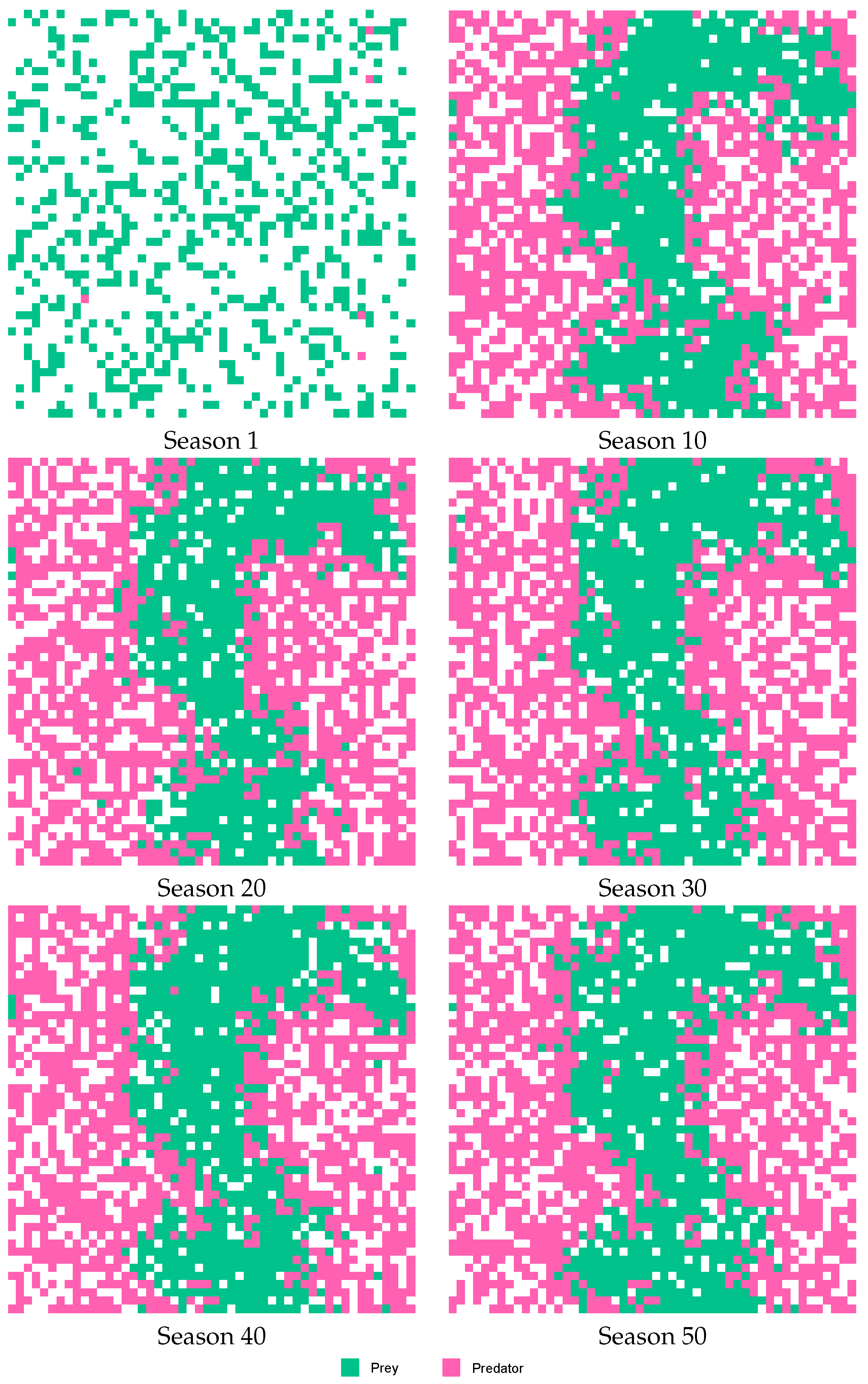
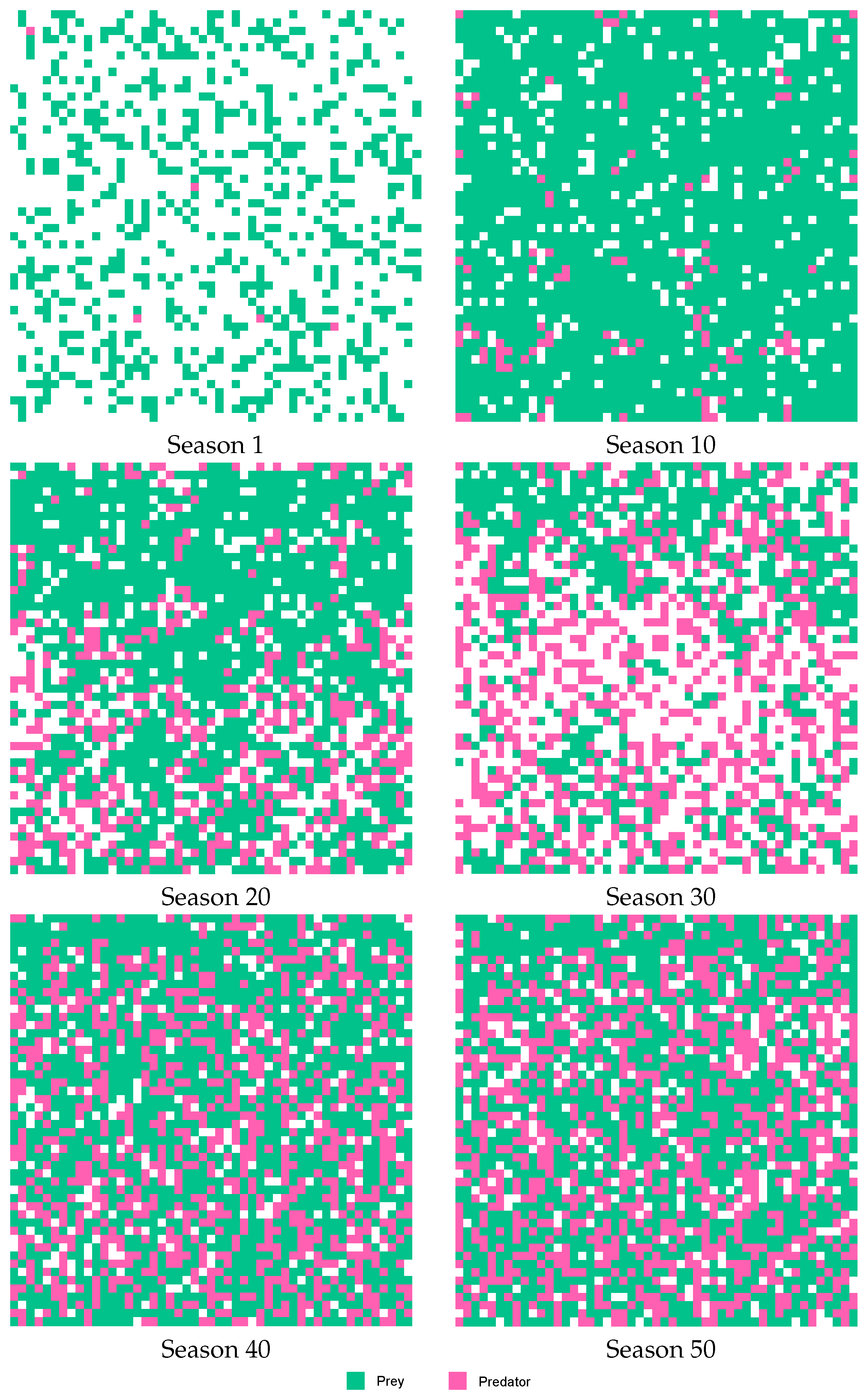
Figure 8 and
Figure 9 describe the behavior of Case E, showing the lattice in six stages of the simulation (Seasons 1, 10, 20, 30, 40 and 50). When considering behavior without using the agent (see
Figure 8), was found that prey kept in the central sector of the lattice, and predators on both sides of the prey. However, when considering the behavior using agents (see
Figure 9), the population of prey and predators were distributed throughout the space of the lattice.
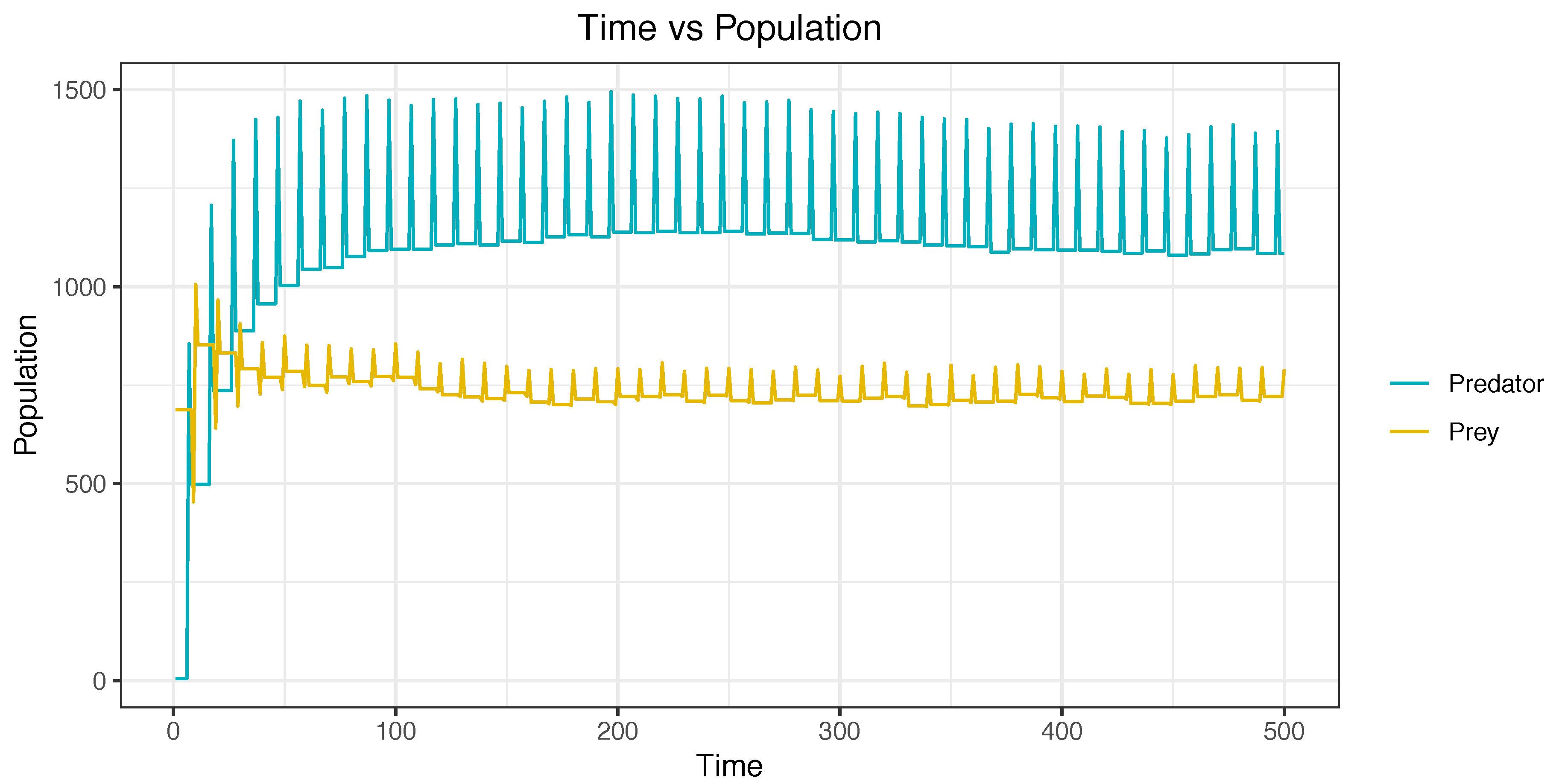
Figure 10 and
Figure 11 describe a simulation from the beginning to the end. The six life cycles of a season were considered.
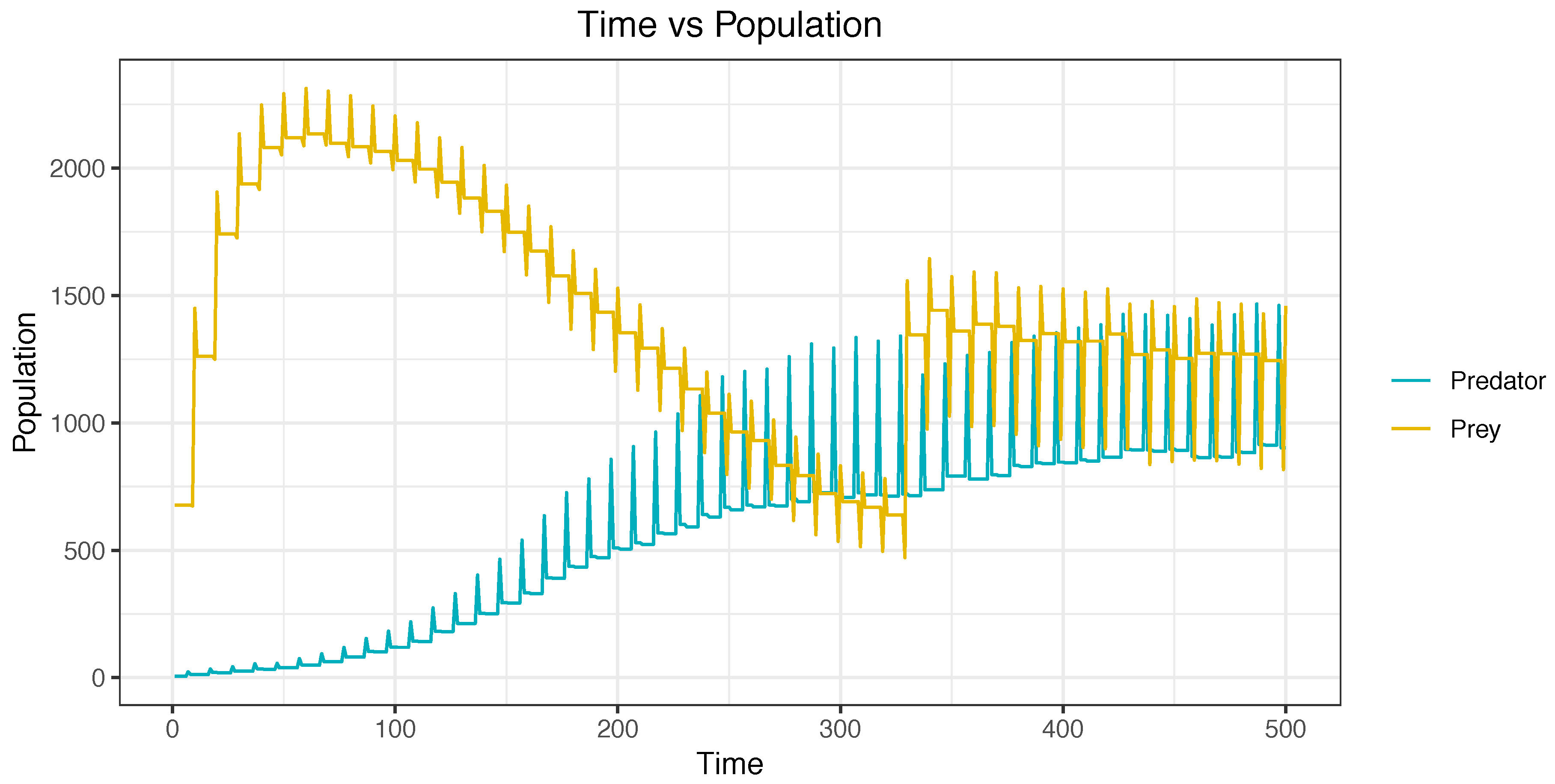
Figure 10 describes a simulation without using agents. Prey and predator populations remained almost static during the simulation. This is easily observable when viewing a straight line in the center of the figure. In contrast,
Figure 11 depicts a simulation using agents. This simulation started with a high population of prey and with a low population of predators. In the figures, it can be observed that, during the simulation, the population of prey decreased, and the population of predators increased. The equilibrium was reached in the final stages of the simulation.
7. Conclusions
In this research, a dynamic prey–predator spatial model was solved using cellular automata. For the movement of the cellular automata, the movement equation of the African buffalo optimization metaheuristics was applied. The results indicate that the prey and predators maintained a population without a considerable variation during the execution of the simulation. In addition, it has been proposed to use a multi-agent system for the resolution of the prey–predator model. In the results obtained, it managed to adjust and maintain a balance of prey and predators, allowing autonomous regulation of the population of prey and predators. The architecture composed of two agents could give real-time descriptions by adjusting the reproduction capacity in real time. As future work, it is proposed to use the equations of movements of various metaheuristics of the literature as well as perform simulations on geo-referential maps.
Author Contributions
Conceptualization, B.A. and F.A.; Data curation, B.A., F.A. and F.Y.; Formal analysis, B.A. and F.A.; Investigation, B.A.; Methodology, B.A.; Project administration, B.A.; Resources, B.A. and F.A.; Software, B.A., F.A. and F.Y.; Supervision, B.A.; Validation, B.A., F.A. and F.Y.; Visualization, F.A.; Writing—original draft, B.A.; and Writing—review and editing, B.A.
Funding
This research received no external funding.
Acknowledgments
Boris Almonacid is supported by Ph.D (h.c) Sonia Alvarez, Chile. Also, we thank the anonymous reviewers for their constructive comments.
Conflicts of Interest
The authors declare no conflict of interest.
Abbreviations
The following abbreviations are used in this manuscript:
| ABO | African Buffalo Optimization |
| MAS | Multi-Agent System |
| GIS | Geographic Information System |
| CA | Cellular Automaton |
References
- Yang, X.S. Nature-Inspired Metaheuristic Algorithms; Luniver Press: Bristol, UK, 2010. [Google Scholar]
- Yang, X.S. Firefly algorithms for multimodal optimization. In Proceedings of the International Symposium on Stochastic Algorithms, Sapporo, Japan, 26–28 October 2009; Springer: Berlin, Germany, 2009; pp. 169–178. [Google Scholar]
- Yang, X.S.; Deb, S. Cuckoo search via Lévy flights. In Proceedings of the World Congress on Nature & Biologically Inspired Computing, NaBIC 2009, Coimbatore, India, 9–11 December 2009; IEEE: New York, NY, USA, 2009; pp. 210–214. [Google Scholar]
- Yang, X.S. A new metaheuristic bat-inspired algorithm. In Nature Inspired Cooperative Strategies for Optimization (NICSO 2010); Springer: Berlin/Heidelberg, Germany, 2010; pp. 65–74. [Google Scholar]
- Odili, J.B.; Kahar, M.N.M. African Buffalo Optimization (ABO): A New Meta-Heuristic Algorithm. J. Adv. Appl. Sci. 2015, 3, 101–106. [Google Scholar]
- Odili, J.B.; Kahar, M.N.M.; Anwar, S. African Buffalo Optimization: A Swarm-Intelligence Technique. Procedia Comput. Sci. 2015, 76, 443–448. [Google Scholar] [CrossRef]
- Yang, X.S. Flower pollination algorithm for global optimization. In Proceedings of the 11th International Conference, UCNC 2012, Orléan, France, 3–7 September 2012; Springer: Berlin, Germany, 2012; pp. 240–249. [Google Scholar]
- Salcedo-Sanz, S.; Del Ser, J.; Landa-Torres, I.; Gil-López, S.; Portilla-Figueras, J. The coral reefs optimization algorithm: A novel metaheuristic for efficiently solving optimization problems. Sci. World J. 2014, 2014, 739768. [Google Scholar] [CrossRef] [PubMed]
- Geem, Z.W.; Kim, J.H.; Loganathan, G. A new heuristic optimization algorithm: Harmony search. Simulation 2001, 76, 60–68. [Google Scholar] [CrossRef]
- Hamadneh, N.; Khan, W.; Tilahun, S. Optimization of microchannel heat sinks using prey-predator algorithm and artificial neural networks. Machines 2018, 6, 26. [Google Scholar] [CrossRef]
- Martínez-Molina, M.; Moreno-Armendáriz, M.A.; Cruz-Cortés, N.; Mora, J.C.S.T. Modeling prey-predator dynamics via particle swarm optimization and cellular automata. In Proceedings of the Mexican International Conference on Artificial Intelligence, Puebla, Mexico, 26 November–4 December 2011; Springer: Berlin/Heidelberg, Germany, 2011; pp. 189–200. [Google Scholar]
- Molina, M.M.; Moreno-Armendariz, M.A.; Cruz-Cortes, N.; Mora, J.C.S.T. Prey-Predator dynamics and swarm intelligence on a cellular automata model. Appl. Comput. Math. 2012, 11, 243–256. [Google Scholar]
- Molina, M.M.; Moreno-Armendáriz, M.A.; Mora, J.C.S.T. On the spatial dynamics and oscillatory behavior of a predator-prey model based on cellular automata and local particle swarm optimization. J. Theor. Biol. 2013, 336, 173–184. [Google Scholar] [CrossRef]
- Molina, M.M.; Moreno-Armendáriz, M.A.; Mora, J.C.S.T. Analyzing the spatial dynamics of a prey–predator lattice model with social behavior. Ecol. Complex. 2015, 22, 192–202. [Google Scholar] [CrossRef]
- Wolfram, S. Theory and Applications of Cellular Automata; World Scientific: Singapore, 1986; Volume 1. [Google Scholar]
- Kari, J. Theory of cellular automata: A survey. Theor. Comput. Sci. 2005, 334, 3–33. [Google Scholar] [CrossRef]
- Abrams, P.A.; Matsuda, H. Prey adaptation as a cause of predator-prey cycles. Evolution 1997, 51, 1742–1750. [Google Scholar] [CrossRef]
- Drossel, B.; Higgs, P.G.; McKane, A.J. The influence of predator–prey population dynamics on the long-term evolution of food web structure. J. Theor. Biol. 2001, 208, 91–107. [Google Scholar] [CrossRef] [PubMed]
- Pang, P.Y.; Wang, M. Strategy and stationary pattern in a three-species predator–prey model. J. Differ. Equ. 2004, 200, 245–273. [Google Scholar] [CrossRef]
- Wang, M. Stationary patterns for a prey–predator model with prey-dependent and ratio-dependent functional responses and diffusion. Phys. D Nonlinear Phenom. 2004, 196, 172–192. [Google Scholar] [CrossRef]
- Durrett, R.; Mayberry, J. Evolution in predator–prey systems. Stoch. Process. Appl. 2010, 120, 1364–1392. [Google Scholar] [CrossRef]
- Costa, M.; Hauzy, C.; Loeuille, N.; Méléard, S. Stochastic eco-evolutionary model of a prey-predator community. J. Math. Biol. 2016, 72, 573–622. [Google Scholar] [CrossRef] [PubMed]
- Abrams, P.A. The evolution of predator-prey interactions: Theory and evidence. Annu. Rev. Ecol. Syst. 2000, 31, 79–105. [Google Scholar] [CrossRef]
- Wolfram, S. Universality and complexity in cellular automata. Phys. D Nonlinear Phenom. 1984, 10, 1–35. [Google Scholar] [CrossRef]
- Batty, M.; Xie, Y.; Sun, Z. Modeling urban dynamics through GIS-based cellular automata. Comput. Environ. Urban Syst. 1999, 23, 205–233. [Google Scholar] [CrossRef]
- White, R.; Engelen, G. Cellular automata and fractal urban form: A cellular modelling approach to the evolution of urban land-use patterns. Environ. Plan. A 1993, 25, 1175–1199. [Google Scholar] [CrossRef]
- Fates, N. Stochastic cellular automata solutions to the density classification problem. Theory Comput. Syst. 2013, 53, 223–242. [Google Scholar] [CrossRef]
- Hu, W.; Wang, H.; Peng, C.; Wang, H.; Liang, H.; Du, B. An outer–inner fuzzy cellular automata algorithm for dynamic uncertainty multi-project scheduling problem. Soft Comput. 2015, 19, 2111–2132. [Google Scholar] [CrossRef]
- Tralic, D.; Rosin, P.L.; Sun, X.; Grgic, S. Detection of duplicated image regions using cellular automata. In Proceedings of the 2014 International Conference on Systems, Signals and Image Processing (IWSSIP), Dubrovnik, Croatia, 12–15 May 2014; IEEE: New York, NY, USA, 2014; pp. 167–170. [Google Scholar]
- Afshar, M.; Zaheri, M.; Kim, J. Improving the Efficiency of Cellular Automata for Sewer Network Design Optimization Problems Using Adaptive Refinement. Procedia Eng. 2016, 154, 1439–1447. [Google Scholar] [CrossRef]
- Kotyrba, M.; Volna, E.; Bujok, P. Unconventional modelling of complex system via cellular automata and differential evolution. Swarm Evol. Comput. 2015, 25, 52–62. [Google Scholar] [CrossRef]
- Toffoli, T.; Margolus, N.H. Invertible cellular automata: A review. Phys. D Nonlinear Phenom. 1990, 45, 229–253. [Google Scholar] [CrossRef]
- Mitchell, M.; Crutchfield, J.P.; Das, R. Evolving cellular automata with genetic algorithms: A review of recent work. In Proceedings of the First International Conference on Evolutionary Computation and Its Applications (EvCA’96), Moscow, Russia, 24–27 June 1996. [Google Scholar]
- Santé, I.; García, A.M.; Miranda, D.; Crecente, R. Cellular automata models for the simulation of real-world urban processes: A review and analysis. Landsc. Urban Plan. 2010, 96, 108–122. [Google Scholar] [CrossRef]
- Pandey, G.; Rao, K.R.; Mohan, D. A review of cellular automata model for heterogeneous traffic conditions. In Traffic and Granular Flow’13; Springer: Berlin, Germany, 2015; pp. 471–478. [Google Scholar]
- Boccara, N.; Roblin, O.; Roger, M. Automata network predator-prey model with pursuit and evasion. Phys. Rev. E 1994, 50, 4531. [Google Scholar] [CrossRef]
- Durrett, R.; Levin, S. Spatial aspects of interspecific competition. Theor. Popul. Biol. 1998, 53, 30–43. [Google Scholar] [CrossRef] [PubMed]
- Chen, Q.; Mynett, A.E. Effects of cell size and configuration in cellular automata based prey–predator modelling. Simul. Model. Pract. Theory 2003, 11, 609–625. [Google Scholar] [CrossRef]
- Arashiro, E.; Tomé, T. The threshold of coexistence and critical behaviour of a predator–prey cellular automaton. J. Phys. A Math. Theor. 2007, 40, 887. [Google Scholar] [CrossRef]
- Farina, F.; Dennunzio, A. A predator-prey cellular automaton with parasitic interactions and environmental effects. Fundam. Inf. 2008, 83, 337–353. [Google Scholar]
- Glushko, R.J.; Tenenbaum, J.M.; Meltzer, B. An XML framework for agent-based E-commerce. Commun. ACM 1999, 42, 106–107. [Google Scholar] [CrossRef]
- Maes, P.; Guttman, R.H.; Moukas, A.G. Agents that buy and sell. Commun. ACM 1999, 42, 81–82. [Google Scholar] [CrossRef]
- Ying, W.; Dayong, S. Multi-agent framework for third party logistics in E-commerce. Expert Syst. Appl. 2005, 29, 431–436. [Google Scholar] [CrossRef]
- Gascueña, J.M.; Fernández-Caballero, A. An agent-based intelligent tutoring system for enhancing e-learning/e-teaching. Int. J. Inst. Technol. Distance Learn. 2005, 2, 11–24. [Google Scholar]
- Mao, X.; Li, Z. Agent based affective tutoring systems: A pilot study. Comput. Educ. 2010, 55, 202–208. [Google Scholar] [CrossRef]
- Jara-Roa, D.; Valdiviezo-Díaz, P.; Agila-Palacios, M.; Sarango-Lapo, C.; Rodriguez-Artacho, M. An adaptive multi-agent based architecture for engineering education. In Proceedings of the 2010 IEEE Education Engineering (EDUCON), Madrid, Spain, 14–16 April 2010; IEEE: New York, NY, USA, 2010; pp. 217–222. [Google Scholar]
- Mathieu, P.; Secq, Y. Environment updating and agent scheduling policies in agent-based simulators. In Proceedings of the 4th International Conference on Agents and Artificial Intelligence (ICAART), Vilamoura, Portugal, 6–8 February 2012; pp. 170–175. [Google Scholar]
- Rihawi, O.; Secq, Y.; Mathieu, P. Effective distribution of large scale situated agent-based simulations. In Proceedings of the 6th International Conference on Agents and Artificial Intelligence, Angers, France, 6–8 March 2014; pp. 312–319. [Google Scholar]
- Hassani, K.; Asgari, A.; Lee, W.S. A case study on collective intelligence based on energy flow. In Proceedings of the 2015 IEEE International Conference on Evolving and Adaptive Intelligent Systems (EAIS), Douai, France, 1–3 December 2015; IEEE: New York, NY, USA, 2015; pp. 1–7. [Google Scholar]
- Karsai, I.; Montano, E.; Schmickl, T. Bottom-up ecology: An agent-based model on the interactions between competition and predation. Lett. Biomath. 2016, 3, 161–180. [Google Scholar] [CrossRef]
- Lütz, A.F.; Cazaubiel, A.; Arenzon, J.J. Cyclic Competition and Percolation in Grouping Predator-Prey Populations. Games 2017, 8, 10. [Google Scholar] [CrossRef]
- Almonacid, B. Simulation of a Dynamic Prey-Predator Spatial Model Based on Cellular Automata Using the Behavior of the Metaheuristic African Buffalo Optimization. In Proceedings of the Natural and Artificial Computation for Biomedicine and Neuroscience, Corunna, Spain, 19–23 June 2017; Springer: Berlin, Germany, 2017; pp. 1–11. [Google Scholar]
- Odili, J.B.; Kahar, M.N.M.; Anwar, S.; Azrag, M.A.K. A comparative study of African Buffalo Optimization and Randomized Insertion Algorithm for asymmetric Travelling Salesman’s Problem. In Proceedings of the 2015 4th International Conference on Software Engineering and Computer Systems (ICSECS), Kuantan, Malaysia, 19–21 August 2015; IEEE: New York, NY, USA, 2015; pp. 90–95. [Google Scholar]
- Odili, J.B.; Kahar, M.N.M. Numerical Function Optimization Solutions Using the African Buffalo Optimization Algorithm (ABO). Br. J. Math. Comput. Sci. 2015, 10, 1–12. [Google Scholar] [CrossRef]
- Odili, J.B.; Mohmad Kahar, M.N. Solving the Traveling Salesman’s Problem Using the African Buffalo Optimization. Comput. Intell. Neurosci. 2016, 2016, 3. [Google Scholar] [CrossRef]
- Odili, J.B.; Kahar, M.N.; Noraziah, A. Solving Traveling Salesman’s Problem Using African Buffalo Optimization, Honey Bee Mating Optimization & Lin-Kerninghan Algorithms. World Appl. Sci. J. 2016, 34, 911–916. [Google Scholar]
- Odili, J.B.; Kahar, M.N.; Noraziah, A.; Odili, E.A. African Buffalo Optimization and the randomized insertion algorithm for the asymmetric travelling salesman’s problems. J. Theor. Appl. Inf. Technol. 2016, 87, 356–364. [Google Scholar]
- Odili, J.B.; Nizam, M.; Kahar, M.; Noraziah, A. African Buffalo Optimization approach to the design of PID controller in automatic voltage regulator system. In Proceedings of the National Conference for Postgraduate Research, Gambang, Malaysia, 24–25 September 2016; pp. 641–648. [Google Scholar]
- Odili, J.B.; Noraziah, A. African Buffalo Optimization for global optimization. Curr. Sci. 2018, 114, 627–636. [Google Scholar] [CrossRef]
Figure 1.
Cellular automata details.
Figure 1.
Cellular automata details.
Figure 2.
Lattice in form of a torus.
Figure 2.
Lattice in form of a torus.
Figure 3.
Lattice definition.
Figure 3.
Lattice definition.
Figure 4.
Cellular automata with African buffalo optimization.
Figure 4.
Cellular automata with African buffalo optimization.
Figure 5.
Season—life cycle.
Figure 5.
Season—life cycle.
Figure 6.
Architecture of dynamic prey–predator spatial model with MAS, CA and ABO.
Figure 6.
Architecture of dynamic prey–predator spatial model with MAS, CA and ABO.
Figure 7.
Moore neighborhood or radius: (left) prey; and (right) predator.
Figure 7.
Moore neighborhood or radius: (left) prey; and (right) predator.
Figure 8.
Population behavior without using agents.
Figure 8.
Population behavior without using agents.
Figure 9.
Population behavior using agents.
Figure 9.
Population behavior using agents.
Figure 10.
Simulation from the beginning to the end without using agents—Case E.
Figure 10.
Simulation from the beginning to the end without using agents—Case E.
Figure 11.
Simulation from beginning to end using agents—Case E.
Figure 11.
Simulation from beginning to end using agents—Case E.
Table 1.
Abbreviations used in the dynamic prey–predator spatial model parameters.
Table 1.
Abbreviations used in the dynamic prey–predator spatial model parameters.
| | Parameter | Abbreviation | Range |
|---|
| Prey | Initial density | Y | |
| (glass) | Reproductive capacity | | |
| | Radius reproduction neighborhood | | |
| | Intraspecific competition coefficient | | |
| | Radius competition neighborhood | | |
| | Number of prey in the neighborhood | | |
| Predator | ABO—Initial density | N | |
| (buffaloes) | Reproductive capacity | | |
| | Radius reproduction neighborhood | | |
| | Radius update | | |
| | ABO—Learning factor | | |
| | ABO—Learning factor | | |
| | ABO—Lambda | | and |
Table 2.
Dynamic prey–predator spatial model parameters.
Table 2.
Dynamic prey–predator spatial model parameters.
| Prey | Value | Predator | Value |
|---|
| Initial density | 1000 | Initial density | 5 |
| Reproductive capacity | 1 | Reproductive capacity | 3 |
| Radius reproduction neighborhood | 3 | Radius reproduction neighborhood | 1 |
| Intraspecific competition coefficient | 0.05 | Radius update | 1 |
| Radius competition neighborhood | 3 | | |
Table 3.
African buffalo optimization metaheuristic parameters.
Table 3.
African buffalo optimization metaheuristic parameters.
| Parameter | Case A | Case B | Case C | Case D | Case E |
|---|
| 1 | 2 | 3 | 4 | 5 |
| 1 | 2 | 3 | 4 | 5 |
| 0.5 | 0.5 | 0.5 | 0.5 | 0.5 |
Table 4.
Simulation carried out without using agents—Case A.
Table 4.
Simulation carried out without using agents—Case A.
| ID | ID-S | ID-SS | Name-SS | ID-M | N-Prey | N-Predator |
|---|
| 1 | 1 | 1 | Intraspecific Competition | - | 674 | 5 |
| 2 | 1 | 2 | Migration | 1 | 674 | 5 |
| 3 | 1 | 3 | Migration | 2 | 674 | 5 |
| 4 | 1 | 4 | Migration | 3 | 674 | 5 |
| 5 | 1 | 5 | Migration | 4 | 674 | 5 |
| 6 | 1 | 6 | Migration | 5 | 674 | 5 |
| 7 | 1 | 7 | Reproduction of Predators | - | 674 | 986 |
| 8 | 1 | 8 | Death of Predators | - | 674 | 569 |
| 9 | 1 | 9 | Predation | - | 412 | 569 |
| 10 | 1 | 10 | Reproduction of Preys | - | 873 | 569 |
| 11 | 50 | 1 | Intraspecific Competition | - | 72 | 1327 |
| 12 | 50 | 2 | Migration | 1 | 72 | 1327 |
| 13 | 50 | 3 | Migration | 2 | 72 | 1327 |
| 14 | 50 | 4 | Migration | 3 | 72 | 1327 |
| 15 | 50 | 5 | Migration | 4 | 72 | 1327 |
| 16 | 50 | 6 | Migration | 5 | 72 | 1327 |
| 17 | 50 | 7 | Reproduction of Predators | - | 72 | 2043 |
| 18 | 50 | 8 | Death of Predators | - | 72 | 1332 |
| 19 | 50 | 9 | Predation | - | 72 | 1332 |
| 20 | 50 | 10 | Reproduction of Preys | - | 80 | 1332 |
Table 5.
Simulation carried out without using agents—Case B.
Table 5.
Simulation carried out without using agents—Case B.
| ID | ID-S | ID-SS | Name-SS | ID-M | N-Prey | N-Predator |
|---|
| 1 | 1 | 1 | Intraspecific Competition | - | 94 | 1339 |
| 2 | 1 | 2 | Migration | 1 | 94 | 1339 |
| 3 | 1 | 3 | Migration | 2 | 94 | 1339 |
| 4 | 1 | 4 | Migration | 3 | 94 | 2088 |
| 5 | 1 | 5 | Migration | 4 | 94 | 1343 |
| 6 | 1 | 6 | Migration | 5 | 87 | 1343 |
| 7 | 1 | 7 | Reproduction of Predators | - | 105 | 1343 |
| 8 | 1 | 8 | Death of Predators | - | 87 | 1343 |
| 9 | 1 | 9 | Predation | - | 87 | 1343 |
| 10 | 1 | 10 | Reproduction of Preys | - | 87 | 1343 |
| 11 | 50 | 1 | Intraspecific Competition | - | 84 | 1323 |
| 12 | 50 | 2 | Migration | 1 | 84 | 1323 |
| 13 | 50 | 3 | Migration | 2 | 84 | 1323 |
| 14 | 50 | 4 | Migration | 3 | 84 | 1323 |
| 15 | 50 | 5 | Migration | 4 | 84 | 1323 |
| 16 | 50 | 6 | Migration | 5 | 84 | 1323 |
| 17 | 50 | 7 | Reproduction of Predators | - | 84 | 2031 |
| 18 | 50 | 8 | Death of Predators | - | 84 | 1322 |
| 19 | 50 | 9 | Predation | - | 83 | 1322 |
| 20 | 50 | 10 | Reproduction of Preys | - | 93 | 1322 |
Table 6.
Simulation carried out without using agents—Case C.
Table 6.
Simulation carried out without using agents—Case C.
| ID | ID-S | ID-SS | Name-SS | ID-M | N-Prey | N-Predator |
|---|
| 1 | 1 | 1 | Intraspecific Competition | - | 671 | 5 |
| 2 | 1 | 2 | Migration | 1 | 671 | 5 |
| 3 | 1 | 3 | Migration | 2 | 671 | 5 |
| 4 | 1 | 4 | Migration | 3 | 671 | 5 |
| 5 | 1 | 5 | Migration | 4 | 671 | 5 |
| 6 | 1 | 6 | Migration | 5 | 671 | 5 |
| 7 | 1 | 7 | Reproduction of Predators | - | 671 | 1153 |
| 8 | 1 | 8 | Death of Predators | - | 671 | 666 |
| 9 | 1 | 9 | Predation | - | 365 | 666 |
| 10 | 1 | 10 | Reproduction of Preys | - | 766 | 666 |
| 11 | 50 | 1 | Intraspecific Competition | - | 18 | 1367 |
| 12 | 50 | 2 | Migration | 1 | 18 | 1367 |
| 13 | 50 | 3 | Migration | 2 | 18 | 1367 |
| 14 | 50 | 4 | Migration | 3 | 18 | 1367 |
| 15 | 50 | 5 | Migration | 4 | 18 | 1367 |
| 16 | 50 | 6 | Migration | 5 | 18 | 1367 |
| 17 | 50 | 7 | Reproduction of Predators | - | 18 | 2140 |
| 18 | 50 | 8 | Death of Predators | - | 18 | 1364 |
| 19 | 50 | 9 | Predation | - | 18 | 1364 |
| 20 | 50 | 10 | Reproduction of Preys | - | 21 | 1364 |
Table 7.
Simulation carried out without using agents—Case D.
Table 7.
Simulation carried out without using agents—Case D.
| ID | ID-S | ID-SS | Name-SS | ID-M | N-Prey | N-Predator |
|---|
| 1 | 1 | 1 | Intraspecific Competition | - | 673 | 5 |
| 2 | 1 | 2 | Migration | 1 | 673 | 5 |
| 3 | 1 | 3 | Migration | 2 | 673 | 5 |
| 4 | 1 | 4 | Migration | 3 | 673 | 5 |
| 5 | 1 | 5 | Migration | 4 | 673 | 5 |
| 6 | 1 | 6 | Migration | 5 | 673 | 5 |
| 7 | 1 | 7 | Reproduction of Predators | - | 673 | 931 |
| 8 | 1 | 8 | Death of Predators | - | 673 | 536 |
| 9 | 1 | 9 | Predation | - | 424 | 536 |
| 10 | 1 | 10 | Reproduction of Preys | - | 903 | 536 |
| 11 | 50 | 1 | Intraspecific Competition | - | 102 | 1312 |
| 12 | 50 | 2 | Migration | 1 | 102 | 1312 |
| 13 | 50 | 3 | Migration | 2 | 102 | 1312 |
| 14 | 50 | 4 | Migration | 3 | 102 | 1312 |
| 15 | 50 | 5 | Migration | 4 | 102 | 1312 |
| 16 | 50 | 6 | Migration | 5 | 102 | 1312 |
| 17 | 50 | 7 | Reproduction of Predators | - | 102 | 1962 |
| 18 | 50 | 8 | Death of Predators | - | 102 | 1315 |
| 19 | 50 | 9 | Predation | - | 102 | 1315 |
| 20 | 50 | 10 | Reproduction of Preys | - | 115 | 1315 |
Table 8.
Simulation carried out without using agents—Case E.
Table 8.
Simulation carried out without using agents—Case E.
| ID | ID-S | ID-SS | Name-SS | ID-M | N-Prey | N-Predator |
|---|
| 1 | 1 | 1 | Intraspecific Competition | - | 673 | 5 |
| 2 | 1 | 2 | Migration | 1 | 673 | 5 |
| 3 | 1 | 3 | Migration | 2 | 673 | 5 |
| 4 | 1 | 4 | Migration | 3 | 673 | 5 |
| 5 | 1 | 5 | Migration | 4 | 673 | 5 |
| 6 | 1 | 6 | Migration | 5 | 673 | 5 |
| 7 | 1 | 7 | Reproduction of Predators | - | 673 | 1109 |
| 8 | 1 | 8 | Death of Predators | - | 673 | 638 |
| 9 | 1 | 9 | Predation | - | 379 | 638 |
| 10 | 1 | 10 | Reproduction of Preys | - | 794 | 638 |
| 11 | 50 | 1 | Intraspecific Competition | - | 457 | 1243 |
| 12 | 50 | 2 | Migration | 1 | 457 | 1243 |
| 13 | 50 | 3 | Migration | 2 | 457 | 1243 |
| 14 | 50 | 4 | Migration | 3 | 457 | 1243 |
| 15 | 50 | 5 | Migration | 4 | 457 | 1243 |
| 16 | 50 | 6 | Migration | 5 | 457 | 1243 |
| 17 | 50 | 7 | Reproduction of Predators | - | 457 | 1714 |
| 18 | 50 | 8 | Death of Predators | - | 457 | 1243 |
| 19 | 50 | 9 | Predation | - | 455 | 1243 |
| 20 | 50 | 10 | Reproduction of Preys | - | 505 | 1243 |
Table 9.
Simulation performed using agents—Case A.
Table 9.
Simulation performed using agents—Case A.
| ID | ID-S | ID-SS | Name-SS | ID-M | N-Prey | N-Predator |
|---|
| 1 | 1 | 1 | Intraspecific Competition | - | 672 | 5 |
| 2 | 1 | 2 | Migration | 1 | 672 | 5 |
| 3 | 1 | 3 | Migration | 2 | 672 | 5 |
| 4 | 1 | 4 | Migration | 3 | 672 | 5 |
| 5 | 1 | 5 | Migration | 4 | 672 | 5 |
| 6 | 1 | 6 | Migration | 5 | 672 | 5 |
| 7 | 1 | 7 | Reproduction of Predators | - | 672 | 13 |
| 8 | 1 | 8 | Death of Predators | - | 672 | 8 |
| 9 | 1 | 9 | Predation | - | 668 | 8 |
| 10 | 1 | 10 | Reproduction of Preys | - | 1483 | 8 |
| 11 | 50 | 1 | Intraspecific Competition | - | 1291 | 874 |
| 12 | 50 | 2 | Migration | 1 | 1291 | 874 |
| 13 | 50 | 3 | Migration | 2 | 1291 | 874 |
| 14 | 50 | 4 | Migration | 3 | 1291 | 874 |
| 15 | 50 | 5 | Migration | 4 | 1291 | 874 |
| 16 | 50 | 6 | Migration | 5 | 1291 | 874 |
| 17 | 50 | 7 | Reproduction of Predators | - | 1291 | 1402 |
| 18 | 50 | 8 | Death of Predators | - | 1291 | 871 |
| 19 | 50 | 9 | Predation | - | 875 | 871 |
| 20 | 50 | 10 | Reproduction of Preys | - | 1492 | 871 |
Table 10.
Simulation performed using agents—Case B.
Table 10.
Simulation performed using agents—Case B.
| ID | ID-S | ID-SS | Name-SS | ID-M | N-Prey | N-Predator |
|---|
| 1 | 1 | 1 | Intraspecific Competition | - | 669 | 5 |
| 2 | 1 | 2 | Migration | 1 | 669 | 5 |
| 3 | 1 | 3 | Migration | 2 | 669 | 5 |
| 4 | 1 | 4 | Migration | 3 | 669 | 5 |
| 5 | 1 | 5 | Migration | 4 | 669 | 5 |
| 6 | 1 | 6 | Migration | 5 | 669 | 5 |
| 7 | 1 | 7 | Reproduction of Predators | - | 669 | 15 |
| 8 | 1 | 8 | Death of Predators | - | 669 | 8 |
| 9 | 1 | 9 | Predation | - | 666 | 8 |
| 10 | 1 | 10 | Reproduction of Preys | - | 1483 | 8 |
| 11 | 50 | 1 | Intraspecific Competition | - | 1294 | 874 |
| 12 | 50 | 2 | Migration | 1 | 1294 | 874 |
| 13 | 50 | 3 | Migration | 2 | 1294 | 874 |
| 14 | 50 | 4 | Migration | 3 | 1294 | 874 |
| 15 | 50 | 5 | Migration | 4 | 1294 | 874 |
| 16 | 50 | 6 | Migration | 5 | 1294 | 874 |
| 17 | 50 | 7 | Reproduction of Predators | - | 1294 | 1409 |
| 18 | 50 | 8 | Death of Predators | - | 1294 | 878 |
| 19 | 50 | 9 | Predation | - | 869 | 878 |
| 20 | 50 | 10 | Reproduction of Preys | - | 1489 | 878 |
Table 11.
Simulation performed using agents—Case C.
Table 11.
Simulation performed using agents—Case C.
| ID | ID-S | ID-SS | Name-SS | ID-M | N-Prey | N-Predator |
|---|
| 1 | 1 | 1 | Intraspecific Competition | - | 674 | 5 |
| 2 | 1 | 2 | Migration | 1 | 674 | 5 |
| 3 | 1 | 3 | Migration | 2 | 674 | 5 |
| 4 | 1 | 4 | Migration | 3 | 674 | 5 |
| 5 | 1 | 5 | Migration | 4 | 674 | 5 |
| 6 | 1 | 6 | Migration | 5 | 674 | 5 |
| 7 | 1 | 7 | Reproduction of Predators | - | 674 | 13 |
| 8 | 1 | 8 | Death of Predators | - | 674 | 8 |
| 9 | 1 | 9 | Predation | - | 670 | 8 |
| 10 | 1 | 10 | Reproduction of Preys | - | 1476 | 8 |
| 11 | 50 | 1 | Intraspecific Competition | - | 1296 | 870 |
| 12 | 50 | 2 | Migration | 1 | 1296 | 870 |
| 13 | 50 | 3 | Migration | 2 | 1296 | 870 |
| 14 | 50 | 4 | Migration | 3 | 1296 | 870 |
| 15 | 50 | 5 | Migration | 4 | 1296 | 870 |
| 16 | 50 | 6 | Migration | 5 | 1296 | 870 |
| 17 | 50 | 7 | Reproduction of Predators | - | 1296 | 1404 |
| 18 | 50 | 8 | Death of Predators | - | 1296 | 876 |
| 19 | 50 | 9 | Predation | - | 872 | 876 |
| 20 | 50 | 10 | Reproduction of Preys | - | 1491 | 876 |
Table 12.
Simulation performed using agents—Case D.
Table 12.
Simulation performed using agents—Case D.
| ID | ID-S | ID-SS | Name-SS | ID-M | N-Prey | N-Predator |
|---|
| 1 | 1 | 1 | Intraspecific Competition | - | 673 | 5 |
| 2 | 1 | 2 | Migration | 1 | 673 | 5 |
| 3 | 1 | 3 | Migration | 2 | 673 | 5 |
| 4 | 1 | 4 | Migration | 3 | 673 | 5 |
| 5 | 1 | 5 | Migration | 4 | 673 | 5 |
| 6 | 1 | 6 | Migration | 5 | 673 | 5 |
| 7 | 1 | 7 | Reproduction of Predators | - | 673 | 13 |
| 8 | 1 | 8 | Death of Predators | - | 673 | 8 |
| 9 | 1 | 9 | Predation | - | 670 | 8 |
| 10 | 1 | 10 | Reproduction of Preys | - | 1481 | 8 |
| 11 | 50 | 1 | Intraspecific Competition | - | 1299 | 874 |
| 12 | 50 | 2 | Migration | 1 | 1299 | 874 |
| 13 | 50 | 3 | Migration | 2 | 1299 | 874 |
| 14 | 50 | 4 | Migration | 3 | 1299 | 874 |
| 15 | 50 | 5 | Migration | 4 | 1299 | 874 |
| 16 | 50 | 6 | Migration | 5 | 1299 | 874 |
| 17 | 50 | 7 | Reproduction of Predators | - | 1299 | 1405 |
| 18 | 50 | 8 | Death of Predators | - | 1299 | 876 |
| 19 | 50 | 9 | Predation | - | 875 | 876 |
| 20 | 50 | 10 | Reproduction of Preys | - | 1494 | 876 |
Table 13.
Simulation performed using agents—Case E.
Table 13.
Simulation performed using agents—Case E.
| ID | ID-S | ID-SS | Name-SS | ID-M | N-Prey | N-Predator |
|---|
| 1 | 1 | 1 | Intraspecific Competition | - | 664 | 5 |
| 2 | 1 | 2 | Migration | 1 | 664 | 5 |
| 3 | 1 | 3 | Migration | 2 | 664 | 5 |
| 4 | 1 | 4 | Migration | 3 | 664 | 5 |
| 5 | 1 | 5 | Migration | 4 | 664 | 5 |
| 6 | 1 | 6 | Migration | 5 | 664 | 5 |
| 7 | 1 | 7 | Reproduction of Predators | - | 664 | 15 |
| 8 | 1 | 8 | Death of Predators | - | 664 | 8 |
| 9 | 1 | 9 | Predation | - | 661 | 8 |
| 10 | 1 | 10 | Reproduction of Preys | - | 1483 | 8 |
| 11 | 50 | 1 | Intraspecific Competition | - | 1307 | 868 |
| 12 | 50 | 2 | Migration | 1 | 1307 | 868 |
| 13 | 50 | 3 | Migration | 2 | 1307 | 868 |
| 14 | 50 | 4 | Migration | 3 | 1307 | 868 |
| 15 | 50 | 5 | Migration | 4 | 1307 | 868 |
| 16 | 50 | 6 | Migration | 5 | 1307 | 868 |
| 17 | 50 | 7 | Reproduction of Predators | - | 1307 | 1400 |
| 18 | 50 | 8 | Death of Predators | - | 1307 | 875 |
| 19 | 50 | 9 | Predation | - | 880 | 875 |
| 20 | 50 | 10 | Reproduction of Preys | - | 1494 | 875 |
© 2019 by the authors. Licensee MDPI, Basel, Switzerland. This article is an open access article distributed under the terms and conditions of the Creative Commons Attribution (CC BY) license (http://creativecommons.org/licenses/by/4.0/).


