A Novel Multi-Objective Five-Elements Cycle Optimization Algorithm

Abstract

Inspired by the mechanism of generation and restriction among five elements in Chinese traditional culture, we present a novel Multi-Objective Five-Elements Cycle Optimization algorithm (MOFECO). During the optimization process of MOFECO, we use individuals to represent the elements. At each iteration, we first divide the population into several cycles, each of which contains several individuals. Secondly, for every individual in each cycle, we judge whether to update it according to the force exerted on it by other individuals in the cycle. In the case of an update, a local or global update is selected by a dynamically adjustable probability $P_s$; otherwise, the individual is retained. Next, we perform combined mutation operations on the updated individuals, so that a new population contains both the reserved and updated individuals for the selection operation. Finally, the fast non-dominated sorting method is adopted on the current population to obtain an optimal Pareto solution set. The parameters’ comparison of MOFECO is given by an experiment and also the performance of MOFECO is compared with three classic evolutionary algorithms Non-dominated Sorting Genetic Algorithm II (NSGA-II), Multi-Objective Particle Swarm Optimization algorithm (MOPSO), Pareto Envelope-based Selection Algorithm II (PESA-II) and two latest algorithms Knee point-driven Evolutionary Algorithm (KnEA) and Non-dominated Sorting and Local Search (NSLS) on solving test function sets Zitzler et al’s Test suite (ZDT), Deb et al’s Test suite (DTLZ), Walking Fish Group (WFG) and Many objective Function (MaF). The experimental results indicate that the proposed MOFECO can approach the true Pareto-optimal front with both better diversity and convergence compared to the five other algorithms.

1. Introduction

In real-world applications, commonly Multiple-Objective Optimization (MOO) problems are applied to many situations such as biology, engineering, medical and economics, and so forth [1]. Usually this kind of optimization problem contains multiple objectives which conflict with each other, hence no single optimal solution can be derived. As a result, a set of solutions should be found to trade off the multiple conflicting goals. In the past few decades, Evolutionary Algorithms (EAs), and some population-based meta-heuristic algorithms, have been verified to effectively solve MOO problems and they can also get an optimal Pareto solution set in one run [2]. Therefore, the application of EAs to MOO problems has received considerable attention, which led to the emergence of a new research issue named Multi-Objective Evolutionary Algorithms (MOEAs). Since then, a large number of MOEAs have been developed and widely used, which have become an important research hotspot in evolutionary optimization.

The purpose of researching MOEAs is to make the population converge quickly and widely, and in the meanwhile distribute uniformly in the non-inferior optimal domain of the problem, which means the convergence and diversity of the solution set should be considered simultaneously [3]. In order to achieve these two goals, quite a few well-performed MOEAs have been proposed in the literature. Some of the most representative ones and some of their applications are listed as follows. The Non-dominated Sorting Genetic Algorithm (NSGA)was proposed by Srinivas and Deb [4] and based on this, an improved version Non-dominated Sorting Genetic Algorithm II(NSGA-II) was proposed by Deb et al. [5]. NSGA-II was applied to carry out the integer optimized design of the Methyl Acetate Hydrolysis Process [6]. Zitzler and Thiele proposed the Strength Pareto Evolutionary Algorithms (SPEA) [7] and its improved version Strength Pareto Evolutionary Algorithms II (SPEA-II) [8]. In the optimization of the microgrid energy dispatch, considering the economic costs, energy utilization rate and environmental benefits as multi-objective, the literature [9] established the microgrid energy allocation model and used the PSEA to solve the MOO problem. Corne et al. proposed the Pareto Envelope-based Selection Algorithm (PESA) [10] and its successor Pareto Envelope-based Selection Algorithm II (PESA-II) [11]; Coello et al. proposed the Multi-Objective Particle Swarm Optimization algorithm (MOPSO) [12], which was effectively applied to the design of water distribution systems in Reference [13] and minimizing the total signaling overhead of location management in Long-term Evolution (LTE) networks to solve the signaling overhead in accessing the network in the literature [14]. In recent years, there has also been a considerable amount of newly presented multi-objective optimization algorithms showing their competitiveness in the field of multi-objective optimization. Bili Chen proposed Non-dominated Sorting and Local Search (NSLS) [15], which was used to solve high-dimensional big data and it turned out that NSLS could find a better spread of solutions and better convergence to the true Pareto-optimal front [16]. Bi-Criterion Evolution for Indicator-Based Evolutionary Algorithm (BCE-IBEA) [17] and Multi-Objective Evolutionary Algorithm based on an enhanced Inverted Generational Distance metric (MOEA/IGD-NS) [18], and so forth, also show great potential for solving MOO problems.

In the literature [19], a new Five-Elements Cycle Model (FECM) derived from ancient Chinese philosophy which is based on the Yin-Yang theory and Five Elements (metal, wood, water, fire, earth) is proposed. FECM was established based on the relationship of generation and restriction among the five elements. In FECM, the fitness value of each element is measured by calculating the interaction between elements, and then the element is updated according to its strengths and weaknesses. On the basis of FECM, Five-Elements Cycle Optimization algorithm (FECO) effectively solves both continuous function optimization problems and Traveling Salesman Problems (TSP) [19,20].

In FECM, the population is divided into different cycles and the cycles are independent of each other, which enhances the diversity of the population. While solving MOO problems, we hope that the obtained Pareto solution set has good diversity. Therefore, based on the scheme of FECM, we propose a new meta-heuristic algorithm that can effectively solve MOO problems, named the Multi-Objective Five-Elements Cycle Optimization algorithm (MOFECO).

The rest of this paper is composed of the following 5 parts: Section 2 describes the basic concepts of MOO problems and some related research on MOEAs; Section 3 elaborates the related work of FECO and explains the motivation of the proposed algorithm MOFECO; Section 4 illustrates the principle of the proposed algorithm; Section 5 makes a parameter analysis and then experimentally verifies the performance of MOFECO algorithm compared with the other five MOEAs; Finally, Section 6 draws the conclusion of this paper.

2. Basic Concepts of MOO Problem and Related Research on MOEAs

2.1. Description of Multi-Objective Problems

A Multiple-Objective Optimization(MOO) problem with m target functions and D decision variables (minimizing multi-objective problems) is represented by Equation (1) [21]:

$$\begin{array}{c}\left\{\begin{array}{ccc}min\hfill & Fun(X)\hfill & ={(f_1(X),f_2(X),\dots ,f_m(X))}^T\hfill \\ st.\hfill & g_z(X)\hfill & \ge 0,z=1,2,\dots ,Z\hfill \\ \hfill & h_e(X)\hfill & =0,e=1,2,\dots ,E\hfill \end{array}\right.\hfill \end{array}$$

(1)

where $X=(x_1,x_2,\dots ,x_D)$ represents the D-dimensional control variable, $Fun(X)$ stands for m contradictory objective functions; $g_z(X)\ge 0,z=1,2,\dots ,Z$ defines Z inequality constraints; $h_e(X)=0,e=1,2,\dots ,E$ defines E equality constraint functions. The goal of multi-objective optimization is to find some certain $X^{*}=(x_1^{*},x_2^{*},x_3^{*},\dots ,x_D^{*})$, so that the objectives in $Fun(X^{*})$ can be optimal at the same time under the constraint conditions. However, when solving MOO problems, since the objective functions may be contradictory, it is hardly possible to obtain one single optimal solution that enables every objective function to reach the optimal value, hence some compromise solutions should be made instead. These trade-off solutions enable each objective function to achieve a better condition simultaneously. This type of optimal solution set is called the Pareto solution set or the non-dominated solution set [22]. It was proposed by Vilfredo Pareto in 1896 and is named the Pareto optimal solution. The following basic definitions are often used when it comes to solving MOO problems with MOEAs [23].

Definition 1.

Pareto optimal solution. Given a multi-objective optimization problem shown in Equation (1). If $\forall X\in \Omega$ satisfies the following conditions then $X^{*}\in \Omega$ is the optimal solution:

$$\begin{array}{c}{\wedge }_{i\in r}(f_i(X)=f_i(X^{*}))\hfill \end{array}$$

(2)

Or, there is at least one $j\in \{1,2,\dots ,m\}$, such that:

$$\begin{array}{c}{f}_j(X)>f_j(X^{*})\hfill \end{array}$$

(3)

where $r=(1,2,\dots ,m)$, and Ω satisfies the constraint in Equation (1), which is:

$$\begin{array}{c}\Omega =\{X\in {\mathbb{R}}^n|g_z(X)\ge 0,h_e(X)=0,(z=1,2,\dots ,Z;e=1,2,\dots ,E)\}\hfill \end{array}$$

(4)

Definition 2.

Dominance between individuals. Suppose $X_1$ and $X_2$ are two arbitrary, different individuals in the evolutionary population, if the following two conditions are met, we call $X_1$ dominates $X_2$:

(1) For all sub-objectives, there are $f_r(X_1)\le f_r(X_2)$, $r=(1,2,\dots ,m)$.

(2) There is at least one sub-objective that makes $X_1$ better than $X_2$, that is $\exists j\in \{1,2,\dots ,m\}$, such that $f_j(X_1)<f_j(X_2)$.

We call $X_1$ non-dominated, or not inferior or dominant; $X_2$ is dominated, expressed as $X_1\succ X_2$, where ≻ is the dominant relation.

Definition 3.

Pareto optimal front. Given a MOO problem shown in Equation (1) and its optimal solution set $\left\{X^{*}\right\}$, the Pareto optimal front is defined as:

$$\begin{array}{c}P{F}^{*}=\{Fun(X)=(f_1(X),f_2(X),\dots ,f_m(X))|X\in X^{*}\}\hfill \end{array}$$

(5)

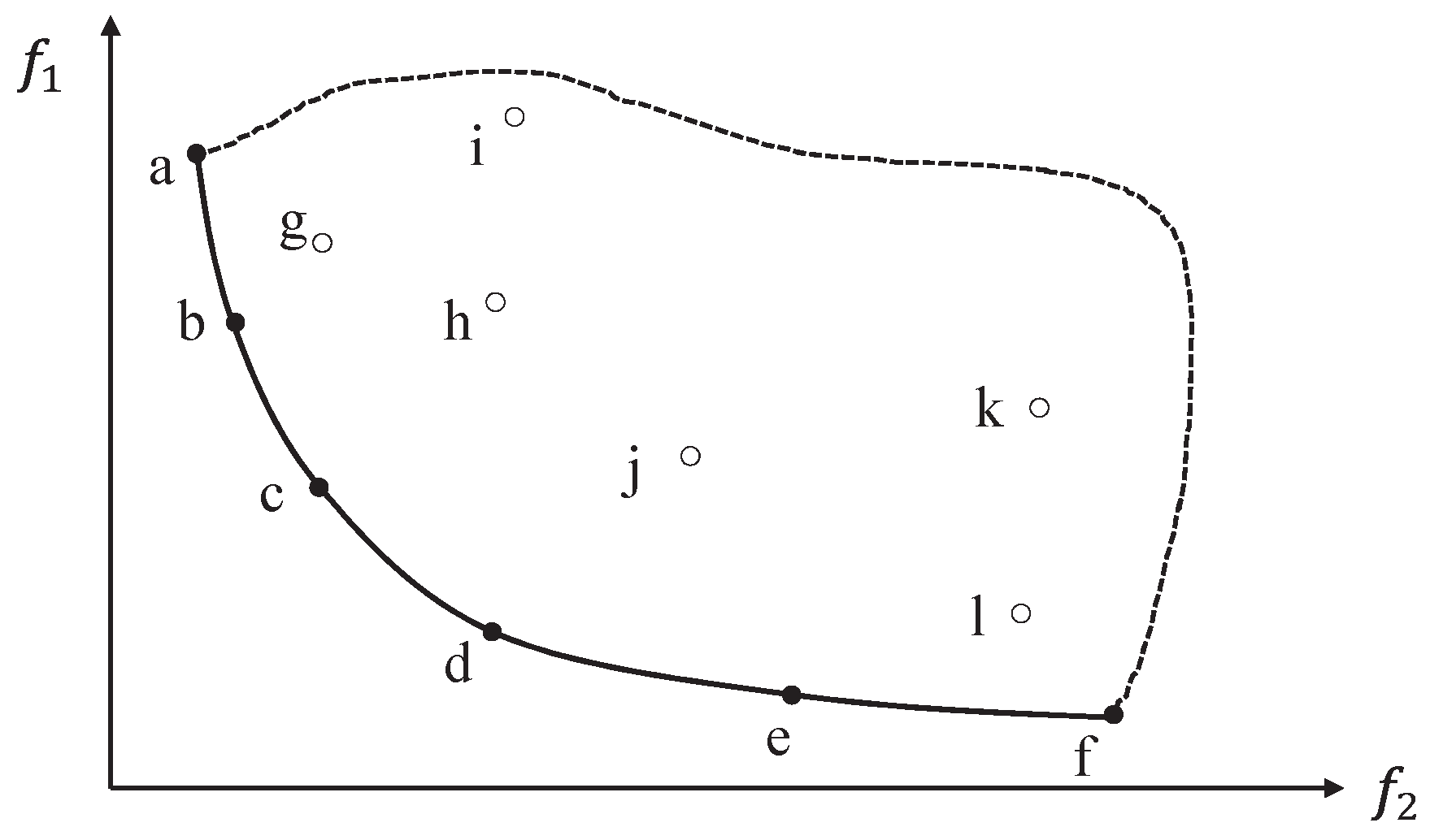
Generally, a set of trade-offs can be obtained for MOO problems, so the most important task in solving a MOO problem is to find a collection of Pareto optimal solutions as close to the true Pareto set as possible [24]. As shown in Figure 1, the solid line denotes the Pareto front of the two optimization objectives $f_1$ and $f_2$. It can be inferred that the Pareto front of a tri-objective problem constitutes a surface and the Pareto front of a many-objective optimization problem (with more than three function objectives) constitutes a hypersurface. In Figure 1, the solid points a, b, c, d, e and f are all on the Pareto front, which are optimal solutions; the hollow points g, h, i, j, k, l fall into the search area, but not on the Pareto front, they are dominated, directly or indirectly by the non-dominated solutions on the Pareto front [25].

2.2. Research on Multi-Objective Evolutionary Algorithms

As early as 1967, Rosenberg mentioned in his doctoral dissertation that genetic search algorithms can solve MOO problems but it was not until 1985 that the first MOEA Vector Evaluated Genetic Algorithm (VEGA) emerged [26]. What really attracts the evolutionary computation world is the series of MOEAs that have been proposed since 1990. The development of MOEAs can be divided into two stages [27].

The first phase was primarily composed of Pareto-based optimization and non-Pareto-based optimization. One of the typical algorithms not based on Pareto dominance was VEGA, which partitioned the population of size P to r sub-populations and each sub-population evolved for different sub-objectives respectively. The superiority of VEGA was that the operation was simple and could be implemented easily, but it was hard to obtain the optimal solution set when the true Pareto Front was non-convex. The other branch was the Pareto-based approach, which was first put forward by Goldberg [28] in 1989 and introduced the Pareto Rank mechanism to implement the operation of selection. The Pareto-based algorithms mainly include Niched-Pareto Genetic Algorithm (NPGA) [29] proposed by Horn and Nafpliotis, Multi-objective Genetic Algorithm (MOGA) [30] proposed by Fonseca and Fleming, and so forth. However, the Pareto-based approach is not universal and it is necessary to choose a method to maintain the diversity of the solution set based on specific optimization problems.

The concept of “external set” was put forward at the second stage. The MOEAs proposed in this period emphasize efficiency and effectiveness. Among them, the typical ones are given as follows. Knowles and Corne [27] proposed the Pareto Archived Evolution Strategy (PAES) series in 1999, Corne et al. [10] brought forward the Pareto Envelope-based Selection Algorithm (PESA) for MOO problems and proposed its improved version PESA-II [11] in 2001 and Deb et al. [5] put forward a non-dominated set sorting method named Non-dominated Sorting Genetic Algorithm (NSGA-II), which compensates the shortcomings of its previous version NSGA [4]. In NSGA-II, in order to reduce the time complexity of the algorithm, a fast sorting method was applied to construct a non-dominated solution set, but it was difficult to find outliers, and may generate search offset when increasing the number of objective functions [25].

To some extent, the classic MOEAs are very mature but the field of evolutionary algorithms is still evolving. In recent years, a large number of split-new MOEAs has appeared. For example, Wagner and Neumann [31] propose a fast Approximation-Guided Evolutionary multi-objective algorithm (AGE-II), which approximate the archive in order to control its size and influence on the runtime, and avoid the shortcomings of Approximation-Guided Evolution (AGE). Bili Chen and Wenhuan Zeng [15] propose the Non-dominated Sorting and Local Search (NSLS) optimization algorithm, which have better diversity in terms of combining the farthest-candidate approach with the non-dominated sorting method to select the new population members. But it easily falls into local optimum on some test problems. Miqing Li et al. put forward the Bi-criterion evolution for IBEA (BCE-IBEA) ([17,32]), it can freely implement the NPC evolution part, which made the approach effectively for those non-Pareto-based algorithm. Y. Tian et al. [18] propose a Multi-Objective Evolutionary Algorithm based on an enhanced Inverted Generational Distance metric (MOEA/IGD-NS), which improves the method of environmental selection. MOEA/IGD-NS uses an enhanced inverted generational distance metric to find non-contributing solutions (termed IGD-NS). In recent years, more and more researchers are turning their attention to many-objective optimization (MaOO) problems. For example, Deb et al. propose the NSGA-III [33,34] using a reference-point-based non-dominated sorting approach in 2014; Xingyi Zhang and Ye Tian et al. put forward a Knee point-driven Evolutionary Algorithm (KnEA) [2] in 2015 and it shows good effectiveness in both solution quality and algorithm complexity. M. Asafuddoula et al. [21] come up with an Improved Decomposition-Based Evolutionary Algorithm (I-DBEA) in 2015, which produces uniformly distributed reference points by systematic sampling and it uses distance measures method to balance the convergence and diversity.

3. Related Work and the Motivation of This Paper

In this section, we first describe the related work of FECO, which was proposed in Reference [19] for solving single-objective problems. Then, we elaborate the motivation of extending FECO to its multi-objective version, Multi-Objective Five-Elements Cycle Optimization algorithm (MOFECO), by which multi-objective problems can be solved.

3.1. Related Work of Five-Elements Cycle Optimization (FECO)

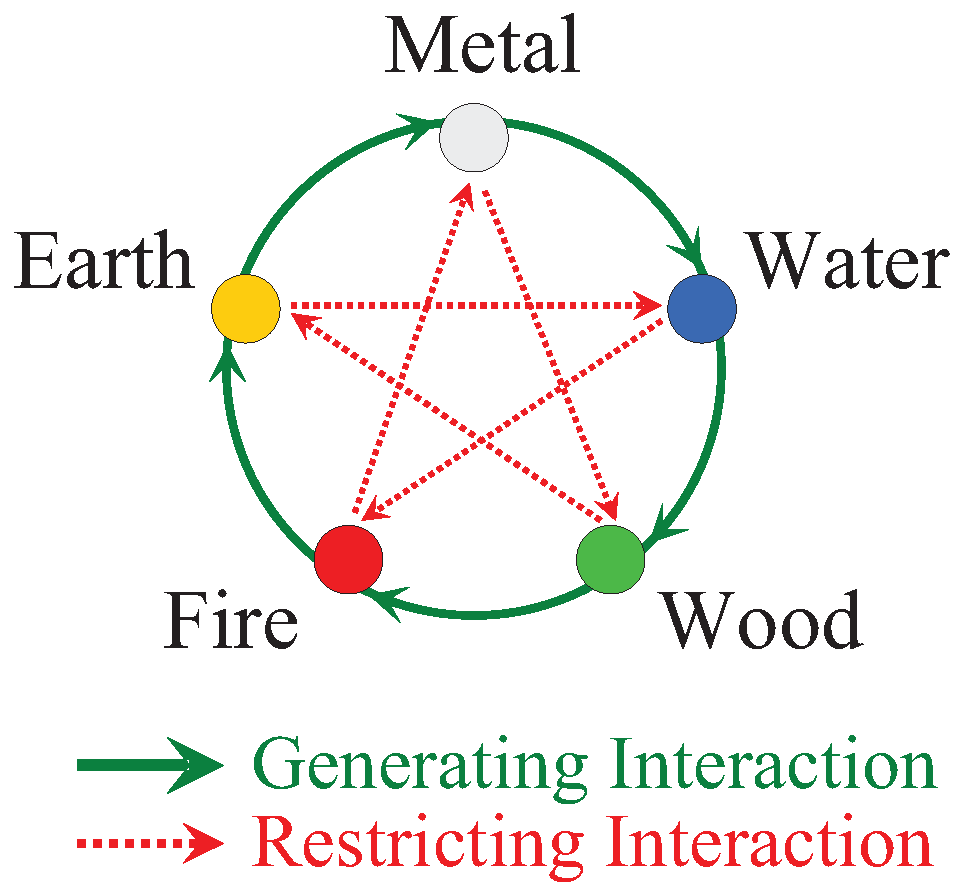
The literature [19] first puts forward the FECM, which draws on the dynamic system equilibrium relationship described by the five elements of ancient Chinese philosophy. The five elements are metal, wood, water, fire and earth. As depicted in Figure 2, there are two main relationships, generating interaction and restricting interaction, between the five elements.

As shown in Figure 2, the outer circle represents the generating interaction: metal produces water, water produces wood, wood produces fire, fire produces earth and earth in its turn produces metal. The generating interaction is analogous to a mother-child relationship, which means children rely on their mother’s nutrition to grow and become strong. The inner circle represents the restricting interaction: wood inhibits earth, earth inhibits water, water inhibits fire, fire inhibits metal and metal in its turn inhibits wood. The restricting interaction as the same as the grandparent-grandchildren relationship, where the grandmother limits the development of grandchildren. Through the generation and restriction, all the elements are mutually restricted and promoted by each other, forming a dynamic equilibrium relationship.

As mentioned above, each element is influenced by the other four in a certain way, and this way is the force relationship between the five elements. The FECM proposed in Reference [19] is described as follows. Suppose a dynamic system consists of the five elements shown in Figure 2. Here we use $X_i(k)$ to represent the i-th element at time k, where $i\in \{1,2,3,4,5\}$ represents the element within each cycle. Each of the elements has its own mass and the force powered by other elements in the same cycle. The mass of the five elements (metal, water, wood, fire, earth) at time k is defined as $M_i(k)$ and the force exerted on the i-th element by the other four elements at time k is denoted by $F_i(k)$, which is corresponding to $M_i(k)$. Each $F_i(k)$ of the elements is composed of four parts (taking the element “metal” for example), the first part is the force of generation from its parent element (earth), denoted by $F_{3\_1}(k)$, and this segment of force is positive because the generation effect from its parent element makes it stronger. The value of $F_{3\_1}(k)$ is determined by the mass of both wood $(M_3(k))$ and water $(M_2(k))$. When $M_2(k)>M_3(k)$, the wood element will become stronger under the generation effect from its parent element. Furthermore, the bigger $M_2(k)$ is, or the smaller $M_3(k)$ is, the greater $F_{3\_1}(k)$ will be. Nevertheless, if $M_2(k)<M_3(k)$, which means wood element was stronger than its parent element, water element will be injured so that $F_{3\_1}(k)$ will reverse. Here, we compute the formula of $F_{3\_1}(k)$ the same as in the literature [19]. The second part is the restriction force from its grandparent element (fire), denoted by $F_{3\_2}(k)$. This segment of force should be negative, because the restriction effect from an element’s grandparent element makes it weaker. In the same way, the value of $F_{3\_2}(k)$ is determined by the mass of both wood $(M_3(k))$ and metal $(M_1(k))$. Similarly, the third part is the generation force to its child element (water), denoted by $F_{3\_3}(k)$ and the fourth segment is the restriction force to its grandchild element (wood), denoted by $F_{3\_4}(k)$. Thus $F_3(k)$ is the weighted sum of the above four segments.

If we extend the wood instance $F_3(k)$ to an arbitrary force $F_i(k)(i\in \{1,2,3,4,5\})$, Equation (6) can be obtained [19]:

$$\begin{array}{c}\left\{\begin{array}{cc}{F}_1(k)\hfill & =w_{gp}·ln[\frac{M_5(k)}{M_1(k)}]-w_{rp}·ln[\frac{M_4(k)}{M_1(k)}]\hfill \\ \hfill & -w_{ga}·ln[\frac{M_1(k)}{M_2(k)}]-w_{ra}·ln[\frac{M_1(k)}{M_3(k)}]\hfill \\ F_2(k)\hfill & =w_{gp}·ln[\frac{M_1(k)}{M_2(k)}]-w_{rp}·ln[\frac{M_5(k)}{M_2(k)}]\hfill \\ \hfill & -w_{ga}·ln[\frac{M_2(k)}{M_3(k)}]-w_{ra}·ln[\frac{M_2(k)}{M_4(k)}]\hfill \\ F_3(k)\hfill & =w_{gp}·ln[\frac{M_2(k)}{M_3(k)}]-w_{rp}·ln[\frac{M_1(k)}{M_3(k)}]\hfill \\ \hfill & -w_{ga}·ln[\frac{M_3(k)}{M_4(k)}]-w_{ra}·ln[\frac{M_3(k)}{M_5(k)}]\hfill \\ F_4(k)\hfill & =w_{gp}·ln[\frac{M_3(k)}{M_4(k)}]-w_{rp}·ln[\frac{M_2(k)}{M_4(k)}]\hfill \\ \hfill & -w_{ga}·ln[\frac{M_4(k)}{M_5(k)}]-w_{ra}·ln[\frac{M_4(k)}{M_1(k)}]\hfill \\ F_5(k)\hfill & =w_{gp}·ln[\frac{M_4(k)}{M_5(k)}]-w_{rp}·ln[\frac{M_3(k)}{M_5(k)}]\hfill \\ \hfill & -w_{ga}·ln[\frac{M_5(k)}{M_1(k)}]-w_{ra}·ln[\frac{M_5(k)}{M_2(k)}]\hfill \end{array}\right.\hfill \end{array}$$

(6)

where each $F_i(k)(i\in \{1,2,3,4,5\})$ of the Equation (6) is composed of the four parts $F_{i\_1}(k)$, $F_{i\_2}(k)$, $F_{i\_3}(k)$, $F_{i\_4}(k)$ described above. The $w_{gp}$, $w_{rp}$, $w_{ga}$, $w_{ra}$ represent weight coefficients.

Considering that the four segments’ forces are not exactly the same, the weighting coefficients $w_{gp}$, $w_{rp}$, $w_{ga}$ and $w_{ra}$ are defined to be positive numerical values in the range of $[0,1]$ [20]. In this paper, we set the same weighting coefficients as in the literature [20]. The mass of each element changes under the generation and restriction force at every iteration as the following Equation (7):

$$\begin{array}{c}{M}_i(k+1)=M_i(k)·f_{\Gamma }(F_i(k)),i\in \{1,2,3,4,5\}\hfill \end{array}$$

(7)

where $f_{\Gamma }(F_i(k))$ is a nonlinear function, which is used to express the variation of elements’ mass under the forces. Extending the five elements to L elements, Equations (6) and (7) can be expressed as Equation (8), which is named FECM, as proposed in Reference [19]:

$$\begin{array}{c}\left\{\begin{array}{c}{F}_i(k)=w_{gp}·ln[\frac{M_{i-1}(k)}{M_i(k)}]-w_{rp}·ln[\frac{M_{i-2}(k)}{M_i(k)}]-w_{ga}·ln[\frac{M_i(k)}{M_{i+1}(k)}]-w_{ra}·ln[\frac{M_i(k)}{M_{i+2}(k)}]\hfill \\ M_i(k+1)=M_i(k)·\frac{2}{1+exp(-F_i(k))}\hfill \end{array}\right.\hfill \end{array}$$

(8)

where $i\in \{1,2,\dots ,L\}$. The subscripts of $M_{i-2}(k)$, $M_{i-1}(k)$, $M_i(k)$, $M_{i+1}(k)$, and $M_{i+2}(k)$ represent the i circulates in the order of $1,2,\dots ,L$.

Based on the FECM described above, Reference [19] proposed FECO for solving single-objective problems and the capability of FECO for solving TSP problems and continuous function optimization problems was verified in Reference [20]. In FECO, the elements are generally divided into q different cycles and each cycle has L elements, where the value of $L\times q$ is equivalent to the population size in the evolution algorithm and each element represents an individual in the population.

3.2. Motivation of This Paper

When optimizing MOO problems, it is necessary to find the Pareto optimal solutions and the ideal optimal solutions distribute evenly on the true Pareto optimal front. That is to say, the main aim of optimizing an MOO problem is to improve diversity and convergence of the solution set. Inspired by FECM, we divide the population into different cycles and the cycles are independent of each other. During the process of evolution, we can perform local search, which means the updated solutions of the individuals are only related to the optimal solution in the cycle to which the individuals belong; and different cycles have different optimal solutions, which shows great merit in terms of population diversity and has certain advantages for solving MOO problems.

4. The Proposed Multi-Objective Five-Elements Cycle Optimization Algorithm

In this paper, a novel MOEA, called the Multi-Objective Five-Elements Cycle Optimization algorithm (MOFECO), is presented. In MOFECO, we introduce the method for constructing a Pareto solution set, the same as in NSGA-II, which used the fast non-dominated sorting and crowded distance method to obtain a Pareto solution set. In the update stage, MOFECO updates the solutions according to the magnitude of the element force, iteratively. Compared to traditional MOEAs such as NSGA-II, the main difference of MOFECO is that it divided the population into different cycles and at each iteration, each cycle performs a local search independently of each other and combines with a global search to make the algorithm quickly and stably converge to the true Pareto set. In the following, the implementation of the proposed MOFECO will be elaborated.

4.1. General Framework of MOFECO

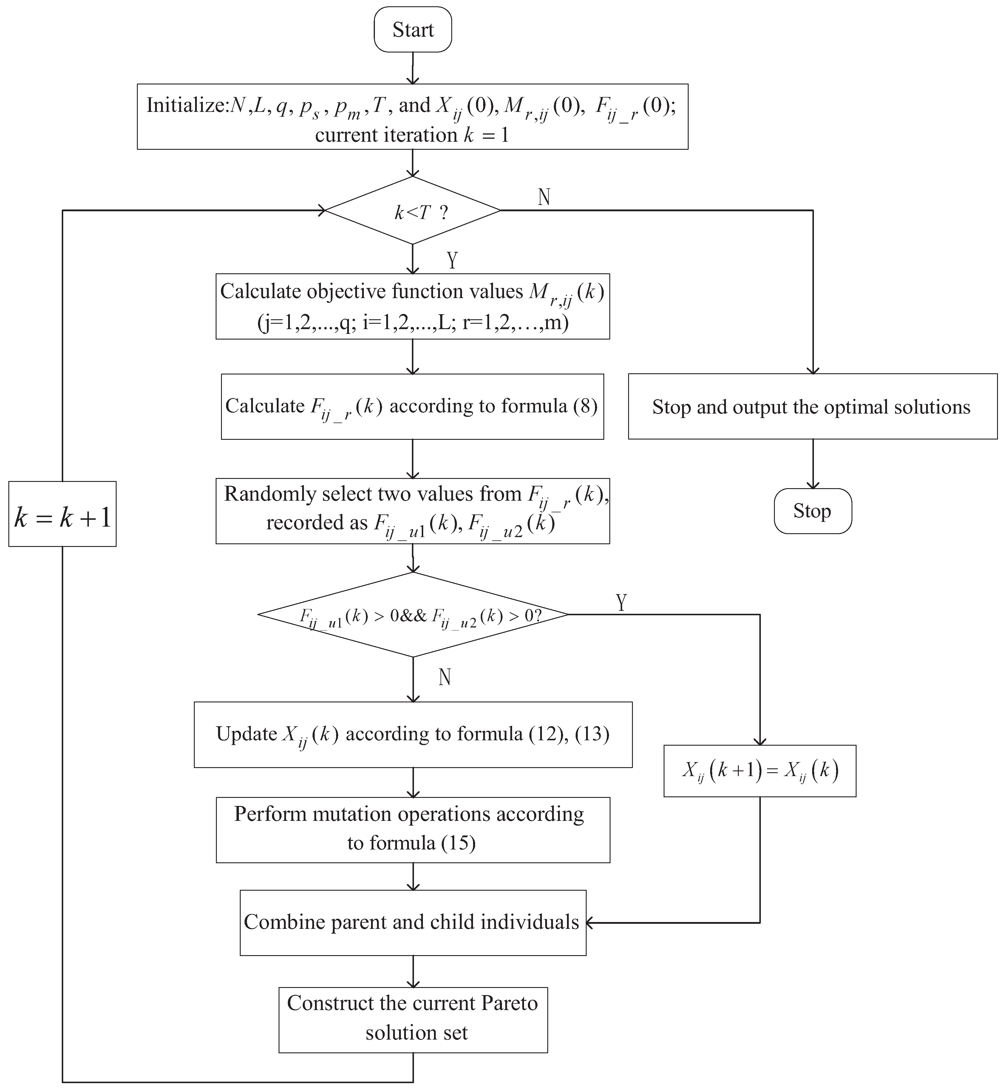
The general framework of MOFECO is similar to most MOEAs, and will be illustrated in the following. First, randomly generate the initial population, which is divided into q cycles according to FECM, and each cycle contains L elements wherein the value of $L\times q$ is the population number N. Then, calculate the objective function values for each individual in the population. Second, determine whether to perform the update operation based on the force of each element. If the current individual satisfies the update condition, the update mode (local-update or global-update) is determined according to the current local-global probability $P_s$, which varies nonlinearly with the number of iterations. Third, the mutation operation is performed according to the mutation probability $P_m$. After the update and mutation operations, we perform the fast non-dominated sorting borrowed from NSGA-II [5] on the current population (including retained and updated individuals), and then select local and global optimal individuals which will be used as the search range for the next-generation individuals when updating. Fourth, we use the methods for the fast non-dominated sorting and crowding distance calculation on the parent and updated population, so as to create the current Pareto optimal solution set. Then, repeats the above process until the maximum number of iterations is reached. The flowchart of MOFECO algorithm is shown in Figure 3. Several parameters are configured in the initialization phase?number of individuals in each cycle L, the number of cycles q, the number of population N, max iteration T, current iteration k, local-global probability $P_s$, mutation probability $P_m$ and weight coefficients $w_{gp}$, $w_{rp}$, $w_{ga}$, $w_{ra}$. In our proposed algorithm, the weight coefficients are set the same as in Reference [20] where $w_{gp}=w_{rp}=w_{ga}=w_{ra}=1$ and we also set the same q and L value as in Reference [20], which proved that these values work the best for the algorithm. Relevant proof will be given in the following parameter comparison experiments in Section 5. Besides, when $k=0$, set the value of $X_{ij}(0)$ and calculate the value of $M_{r,ij}(0)$, $F_{ij\_r}(0)$.

Next, we will describe the proposed algorithm MOFECO in detail in the following parts of this section.

4.2. Expression of Solutions and Population Initialization

Taking the MOO problem in Equation (1) as an example, each solution of $Fun(X)$ corresponds to an element in the FECM. In the proposed algorithm MOFECO, each element represents an individual in the population and the population are divided into q cycles. There are L elements in each cycle, so the population size is $L\times q$. We use $X_{ij}(k)$ to denote the i-th element of the j-th cycle at the k-th iteration and in the population of MOFECO, $X_{ij}(k)$ represents one individual. Since MOFECO is designed for multi-objective problems, one individual corresponds to multiple objective function values. Therefore, we use $M_{r,ij}(k)$ to represent the mass of $X_{ij}(k)$, corresponding to the values of objective function $Fun(X)$, $r\in \{1,2,\dots ,m\}$ that represents m objective functions. In FECM, the force exerted on $X_{ij}(k)$ by other elements in the j-th cycle is related to the element mass. Therefore, in MOFECO, the $X_{ij}(k)$ has multiple forces from the other elements in the j-th cycle, denoted as $F_{ij\_r}(k)$, which is computed by Equation (9).

$$\begin{array}{cc}{F}_{ij\_r}(k)\hfill & =w_{gp}·ln[\frac{M_{r,(i-1)j}(k)}{M_{r,ij}(k)}]-w_{rp}·ln[\frac{M_{r,(i-2)j}(k)}{M_{r,ij}(k)}]\hfill \\ \hfill & -w_{ga}·ln[\frac{M_{r,ij}(k)}{M_{r,(i+1)j}(k)}]-w_{ra}·ln[\frac{M_{r,ij}(k)}{M_{r,(i+2)j}(k)}]\hfill \end{array}$$

(9)

When iteration number $k=0$, we generate $L\times q$ initial individuals $X_{ij}(0)$$(i\in \{1,2,\dots ,L\}$, $j\in \{1,2,\dots ,q\})$ within the feasible range of search space randomly. Then we use FECM to calculate their masses and forces expressed as $M_{r,ij}(0)$, $F_{ij\_r}(0)$, respectively. In the k-th iteration, we firstly use objective functions $M_{r,ij}(k)$ to evaluate $F_{ij\_r}(k)$ by Equation (9). According to FECM, it can be noted that the value of $F_{ij\_r}(k)$ measures the pros and cons of element $X_{ij}(k)$, therefore $F_{ij\_r}(k)$ determines the update pattern of $X_{ij}(k)$. The specific update pattern will be described in detail in Section 4.3.

4.3. Update of Individuals

According to FECM, proposed in Reference [19] and from the expression of solutions in the previous section, we know that the update of individual $X_{ij}(k)$ depends on the corresponding forces $F_{ij\_r}(k)$. From the perspective of system balance and Equation (6), the smaller $M_{r,ij}(k)$ is, the larger $F_{ij\_r}(k)$ is, and since larger force will make the element stronger, so that each element will further converge. Therefore, we can infer that if $F_{ij\_r}(k)$ has a positive value, $X_{ij}(k)$ is a good solution. In this situation, $X_{ij}(k)$ should be reserved. Nonetheless, in MOO problems, the individual $X_{ij}(k)$ corresponds to multiple objective function values, that is, corresponds to multiple forces $F_{ij\_r}(k)$. If we reserved $X_{ij}(k)$ when all $F_{ij\_r}(k)$ have positive value, there are almost no remained individuals. In evolutionary algorithms, however, we usually want to retain 10% to 20% of the current population as the reserved solutions. So, in MOFECO, we update $X_{ij}(k)$ as follows:

$$\begin{array}{c}{X}_{ij}(k+1)=X_{ij}(k)if{F}_{ij\_u1}(k)>0and{F}_{ij\_u2}(k)>0\hfill \end{array}$$

(10)

where $u1$ and $u2$ are randomly chosen from set $\{1,2,\dots m\}$. The above formula shows that two values are randomly selected in the forces of the element to determine whether they are greater than 0; if so, reserve the element.

If the element $X_{ij}(k)$ is subjected to a negative force $F_{ij\_r}(k)$, it indicates that the system expects the element to become weaker and its mass $M_{r,ij}(k)$ must become thinner, which means $X_{ij}(k)$ is probably not a good solution, in that case, the current $X_{ij}(k)$ needs to be updated. According to Equation (10), if at least one of the two randomly selected forces of the element is smaller than 0, the element performs update operation. Then, we can get the update formula as Equation (11):

$$\begin{array}{c}\left\{\begin{array}{cccc}{X}_{ij}(k+1)\hfill & =X_{ij}(k)\hfill & \hfill & if{F}_{ij\_u1}(k)>0and{F}_{ij\_u2}(k)>0\hfill \\ X_{ij}(k+1)\hfill & =X{M}_{ij}(k+1)\hfill & \hfill & others\hfill \end{array}\right.\hfill \end{array}$$

(11)

where $X{M}_{ij}(k+1)$ represents the individual after update and mutation. The specific update operation is designed as follows.

Suppose that the individual $X_{ij}(k)$ is a D-dimensional vector, denoted by $X_{ij,1}(k),X_{ij,2}(k),\dots ,X_{ij,d}(k),\dots ,X_{ij,D}(k)$, and as we hope to generate new solutions in the neighborhood of the better solutions, the improved Particle Swarm Optimization (PSO) [35] algorithm is introduced here. Define the individuals velocity vector $V_{ij}(k)$, whose dimension is also D and expressed as $V_{ij,1}(k),V_{ij,2}(k),\dots ,V_{ij,d}(k),\dots ,V_{ij,D}(k)$, and $X_{ij}(k)$ represents the individual’s position vector. Therefore, when individual $X_{ij}(k)$ satisfies the update condition, it will be updated as follows:

$$\begin{array}{c}\left\{\begin{array}{cccc}{V}_{ij,d}(k+1)\hfill & =\omega \times V_{ij,d}(k)+r_1\times r_s\times (X\_loca{l}_{j,d}(k)-X_{ij,d}(k))\hfill & \hfill & if{r}_m<P_s\hfill \\ V_{ij,d}(k+1)\hfill & =\omega \times V_{ij,d}(k)+r_2\times r_s\times (X\_bes{t}_d(k)-X_{ij,d}(k))\hfill & \hfill & if{r}_m\ge P_s\hfill \end{array}\right.\hfill \end{array}$$

(12)

$$\begin{array}{c}X{C}_{ij,d}(k+1)=X_{ij,d}(k)+V_{ij,d}(k+1)\hfill \end{array}$$

(13)

where $i\in \{1,2,\dots ,L\}$, $j\in \{1,2,\dots ,q\}$, $d\in \{1,2,\dots ,D\}$, representing the number of individuals in one cycle, the number of cycles and the number of dimensions, respectively. And $r_1$ and $r_2$ are constants; $\omega$ represents the inertia weight; $r_s$ is randomly produced in the range of [0, 1]; $P_s$ represents the local-global update probability; $X\_loca{l}_j(k)$ represents the optimal individual in the j-th cycle, that is, after performing fast non-dominated sorting on all individuals in the current population, the individual in the j-th cycle that has the smallest $Rank$ value and maximum crowding distance between two adjacent individuals is recorded as $X\_loca{l}_j(k)$. We randomly select an individual as $X\_best(k)$ among the individuals with $Rank$ value of 1 after the fast non-dominated sorting and crowded distance calculation method in current population. In Equation (13) $X{C}_{ij}(k+1)$ represent the updated individual. It can be seen from Equations (12) and (13) that $X_{ij}(k)$ is updated around the best element of the j-th cycle $X\_loca{l}_j(k)$ under the probability $P_s$. Otherwise, it is updated around the current best optimal solution $X\_best(k)$.

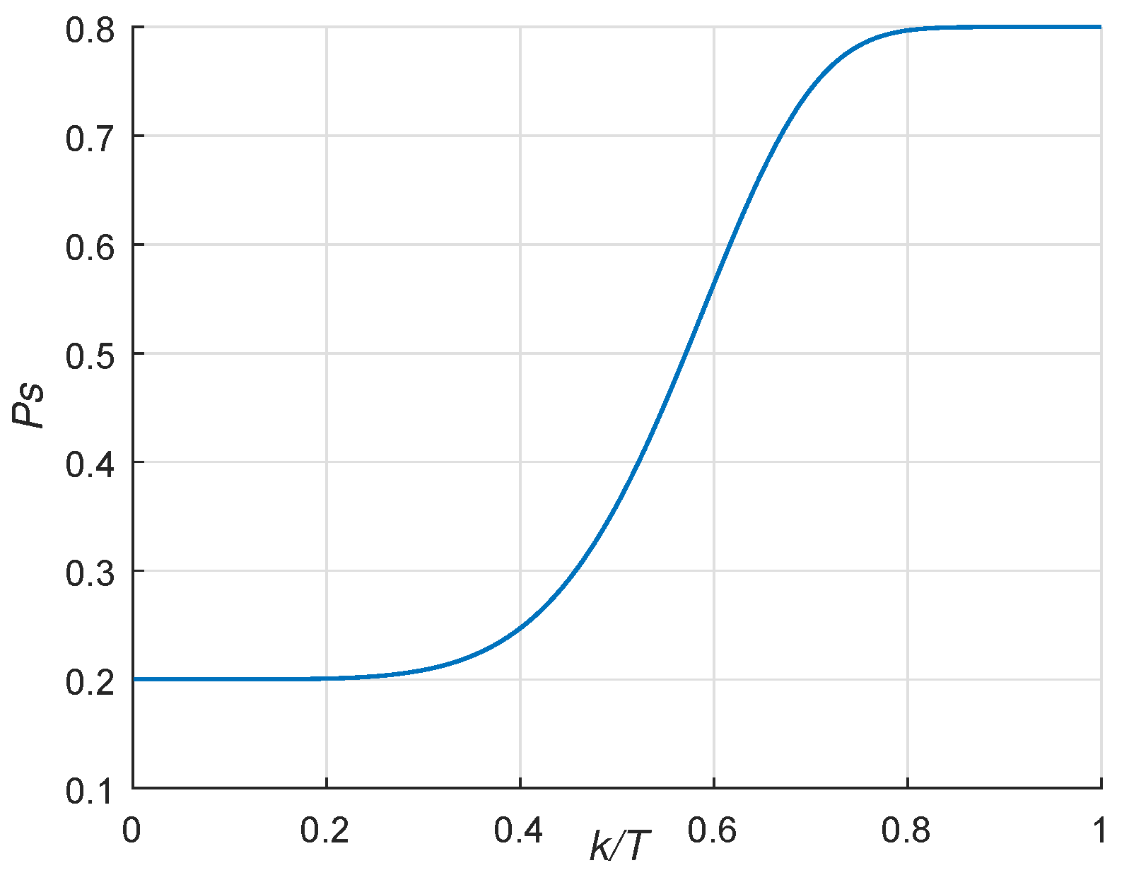
From Equation (12), we can see that large $P_s$ is inclined to exploitation, while small $P_s$ is inclined to exploration. In order to enhance the convergence and flexibility of the proposed algorithm, the value of the probability $P_s$ is not fixed but changes dynamically according to the current iteration number. The variation pattern of $P_s$ with the iteration number is shown in Figure 4. In the initial stage of population evolution, since it is expected that the individuals can converge to the optimal solutions quickly, we assign a small value to $P_s$ so that individuals tend to find updated solutions in the global scope. As the number of iteration increases, we hope to find optimal solutions which are more diverse and distributed, so the value of $P_s$ gradually increases, making individuals tend to perform local search. In this way, the search range of the solutions is dynamically selected according to the phase of evolution, so that the individuals can quickly and effectively approach the best optimal solution set. We define the calculation of $P_s$ as follows:

$$\begin{array}{c}{P}_s=1-(P_{s_{min}}+(P_{s_{max}}-P_{s_{min}})\times exp(-20\times {(k/T)}^6)\hfill \end{array}$$

(14)

where $P_{s_{min}}$ and $P_{s_{max}}$ represent the values of minimum and maximum probability respectively; k is the current number of iterations and T is the maximum iteration.

4.4. Mutation of Individuals

To prevent individuals from falling into local optimum, a mutation operation was introduced in MOFECO. In standard genetic algorithms, the mutations operation often flip each binary bit with a small probability $P_m$, which is used to introduce missing genes into the population to achieve global search of the solution space. To this end, researchers designed a number of mutation operators, such as uniform mutation, non-uniform mutation, Gaussian mutation, Cauchy mutation, polynomial mutation and so on [25]. Reference [36] systematically analyzed the global search ability and local search ability of Gauss distribution, Cauchy distribution and Uniform distribution mutation operator. Theory and practice show that the Gauss distribution operator has strong local search ability, the uniform distribution mutation operator has strong global search ability, and the Cauchy distribution operator has a centered ability of local search and global search.

Hence, we combine these three different mutation operators as follows. In the early stage of evolution, we use the uniform mutation operator to acquire strong global search ability; In the late evolution, we use the Gauss mutation operator to enhance the local search ability of the algorithm; While in the middle of evolution, the Cauchy distribution mutation operator is used to make the algorithm suitable for global and local search. The specific operation is as follows:

$$\begin{array}{c}X{M}_{ij}(k+1)=\left\{\begin{array}{ccc}X{C}_{ij}(k+1)+U(-{\sigma }_1,{\sigma }_1)\hfill & \hfill & if(k+1\le \frac{T}{4})\hfill \\ X{C}_{ij}(k+1)+C(0,{\sigma }_2)\hfill & \hfill & if(\frac{T}{4}<k+1\le \frac{3T}{4})\hfill \\ X{C}_{ij}(k+1)+N(0,{\sigma }_3)\hfill & \hfill & if(\frac{3T}{4}<k+1\le T)\hfill \end{array}\right.\hfill \end{array}$$

(15)

where $X{M}_{ij}(k+1)$ represents the individual after mutation; $U(-{\sigma }_1,{\sigma }_1)$ represents the uniform distribution mutation operator and ${\sigma }_1$ is called the variation domain and usually has ${\sigma }_1=0.1\times (u_p-l_w)$, where $u_p$ and $l_w$ represent the upper and lower bounds of the decision variable; $C(0,{\sigma }_2)$ represents a random number of Cauchy distribution centered at zero and a scale parameter of ${\sigma }_2$; $N(0,{\sigma }_3)$ represents the Gaussian distribution random number.

After the update and mutation operation, a new population is generated, which contains the retained individuals and the updated individuals, and the population size is still N. Then, the fast non-dominated sorting and the crowded distance method in NSGA-II are adopted to sort the new population. The best solution in each cycle and the optimal solution in the new population are picked out as the neighborhood solutions that produce new solutions when the next generation is updated. At the same time, the parent population and the updated individuals are combined to get a new population R, and R is sorted by using fast non-dominated sorting and crowded distance calculation method in NSGA-II. So the solutions with $Rank$ value of 1 and the crowded distance from large to small in the sorted population R are selected as the current Pareto optimal solution set. Then, the above process is repeated until the maximum number of iterations is reached.

5. Simulation Experiment and Result Analysis

In this section, we first compare the parameters of the proposed MOFECO algorithm, including number of cycles q and number of elements L in each cycle, update condition $F_{ij\_r}$, the local-global probability $P_s$ and the mutation methods. Secondly, we analyze the performance of MOFECO by empirically comparing it with three classic MOEAs, namely, NSGA-II [5], MOPSO [12], PESA-II [11] and the two latest algorithms KnEA [2] and NSLS [15]. The experiments were performed on 15 test problems, which were taken from four widely used test benchmarks suites the Zitzler et al’s Test suite (ZDT) [37], the Deb et al’s Test suite (DTLZ) [38], the Walking Fish Group (WFG) [39] and the Many objective Function (MaF) [40]. Among them, the ZDT series are bi-objective functions and the DTLZ series are tri-objective functions and we set the MaF and WFG series as four-objective functions. In terms of experimental configuration, all the implementations are done on a 2.39 GHz Intel(R) Xeon(R) CPU with 32 GB RAM under Microsoft Window 10. MOFECO has been implemented in MATLAB R2016a and for the NSGA-II, MOPSO, PESA-II, KnEA and NSLS, the programs are derived from the platEMO provided by the literature [41].

5.1. Test Problems

Four classic series of test benchmarks, the Zitzler et al’s Test suite (ZDT) proposed by Zitzler et al. [37], the Deb et al.’s Test suite (DTLZ) proposed by Deb et al. [38], the Walking Fish Group (WFG) proposed by Huband et al. [39] and the Many objective Function (MaF) proposed Cheng [40], are used to test the performance of the proposed algorithm. The number of objective functions, the dimensions of control variables and the function features of the test problems are given in

Table 1. ZDT, DTLZ, WFG and MaF decision space dimension.

Test Problem	Dimension D	Number of Objects m	Feature
ZDT1	30	2	Convex function
ZDT2	30	2	Concave function
ZDT4	10	2	Convex function
ZDT6	10	2	Concave function
DTLZ2	12	3	Concave function
DTLZ4	12	3	Concave function
DTZL5	12	3	Concave function
DTLZ6	12	3	Concave function
DTLZ7	22	3	Mixed function
WFG2	13	4	convex function
WFG3	13	4	linear function
WFG4	13	4	concave function
MaF1	13	4	Linear function
MaF2	13	4	Concave function
MaF12	13	4	Concave function

. All of these problems are unconstrained, and the goals of all problems are to minimize the objective functions.

5.2. Performance Metrics

Performance metrics are often used to measure the effectiveness of an algorithm for MOO problems. As we know, the basic aim of multi-objective optimization is to obtain a Pareto set with better convergence, distribution and diversity of the Pareto set. According to whether the performance metrics can measure the convergence, the diversity or both of a solution set, they can be divided into three categories [42], and the following part describes some commonly used performance metrics of the three categories. Here we suppose the true Pareto optimal front is known as $P^{*}$.

(1) Generational Distance ($GD$): $GD$ is used to evaluate the convergence of a solution set, the concept of $GD$ was proposed by Veldhuizen and Lamont [43]. It measures the distance between the obtained non-dominated front P and the true Pareto set $P{F}^{*}$ as:

$$\begin{array}{c}GD=\frac{\sqrt{{\sum }_{i=1}^{\left|P\right|}minDis{(X_i,P{F}^{*})}^2}}{\left|P\right|}\hfill \end{array}$$

(16)

where $minDis(X_i,P{F}^{*})$ represents the minimum Euclidean distance between the obtained solution $X_i$ and the solutions in $P{F}^{*}$, and $\left|P\right|$ is the number of the obtained optimal solutions. $GD$ measures how far these non-dominated solutions X are from those in the true Pareto optimal front $P{F}^{*}$. The smaller the $GD$ value, the closer the Pareto solution set is to the real Pareto frontier and the better convergence the solution set has. If $GD=0$, the solution set is on the real Pareto front, which is the most ideal situation.

(2) Spacing metric ($SP$): The spatial evaluation method $SP$ [44] proposed by Schott is used to evaluate the distribution of individuals in the objective space. The function is defined as follows:

$$\begin{array}{c}SP=\sqrt{\frac{1}{\left|P\right|-1}\sum _{i=1}^{\left|P\right|}{(\overline{d}-d_i)}^2}\hfill \end{array}$$

(17)

$$\begin{array}{c}{d}_i=\underset{j}{min}\left(|f_1^i(X)-f_1^j(X)|+|f_2^i(X)-f_2^j(X)|\right),(i,j=1,2,\dots ,|P|)\hfill \end{array}$$

(18)

where $\overline{d}$ is the average of all $d_i$ and $\left|P\right|$ represents the size of Pareto solutions. A smaller value of $SP$ demonstrates a better distribution of the obtained solution set. Here, $SP=0$ when the algorithm obtained optimal solutions which are completely evenly distributed in the target space.

(3) Spread indicator ($SI$): Wang et al. [42] proposed the spread metric $SI$, which is used for independently evaluating the breadth and the spread of the non-dominated solutions. $SI$ can be defined mathematically as:

$$\begin{array}{c}SI=\frac{{\sum }_{i=1}^{m}d(e_i,P)+{\sum }_{X\in P}|d(X,P)-\overline{d}|}{{\sum }_{i=1}^{m}d(e_i,P)+(|P|-m)\times \overline{d}}\hfill \end{array}$$

(19)

$$\begin{array}{c}d(X,P)=\underset{Y\in P,Y\notin X}{min}\parallel F(X)-F(Y)\parallel \hfill \end{array}$$

(20)

$$\begin{array}{c}\overline{d}=\frac{1}{P}\times \sum _{X\in P}d(X,P)\hfill \end{array}$$

(21)

where P is optimal solution set, m represents the number of objectives, $e_i(i=1,2,\dots ,m)$ are m extreme solutions, which belongs to the set of true Pareto front. As can be seen, a smaller $SI$ means the optimal solution set has a better spread.

(4) Pure diversity ($PD$): $PD$ is used for measuring the diversity of species, it is defined as follows [45]:

$$\begin{array}{c}PD(X)=\underset{s{p}_i\in X}{max}(PD(X-s{p}_i)+d(s{p}_i,X-s{p}_i))\hfill \end{array}$$

(22)

where

$$\begin{array}{c}d(sp,X)=\underset{s{p}_i\in X}{min}(diss(sp,s{p}_i))\hfill \end{array}$$

(23)

Here, $d(s{p}_i,X-s{p}_i)$ represents the dissimilarity d from one species $s{p}_i$ to a community X. The larger the $PD$ value, the better the diversity of the solution set.

(5) Hypervolume ($HV$): $HV$ indicator [46] has become a popular evaluation index because of its good theoretical support. It evaluates the comprehensive performance of MOEAs by calculating the hypervolume value of the space enclosed by the non-dominated solution set and the reference point. The calculation formula is:

$$\begin{array}{c}HV=\lambda \left({\cup }_{i=1}^{\left|P\right|}{v}_i\right)\hfill \end{array}$$

(24)

where $\lambda$ represents the Lebesgue measure, $v_i$ represents the hypervolume formed by the reference point and the non-dominated individual and P represents the optimal solution set. Note that a larger $HV$ denotes a better performance of the algorithm.

(6) Inverted Generational Distance ($IGD$): The $IGD$ [47] is defined as:

$$\begin{array}{c}IGD(P{F}^{*},P)=\frac{{\sum }_{x\in P{F}^{*}}mindis(X,P)}{|P{F}^{*}|}\hfill \end{array}$$

(25)

where $P{F}^{*}$ denotes the uniformly distributed true solutions along the Pareto front. P represents an approximation to the Pareto front. $mindis(X,P)$ denotes the minimum Euclidean distance between the solution X and the solutions in P. we can see that the smaller the $IGD$ value is, the better convergence and diversity of the Pareto optimal set has.

5.3. Parameter Analysis and Comparison Experiments of MOFECO

This section mainly analyzes and compares the parameter in proposed MOFECO include L, q, $F_{ij\_r}$, $P_s$ and mutation methods.

In the comparison experiments, one parameter is varied at a time and the other parameters are fixed to the best parameters which are set as the same as Equations (11), (14) and (15). The common parameter settings in the experiment are shown in

Table 2. Experimental parameters.

Parameters	Values
N	100
T	1000
L	5
q	20
${\mathit{r}}_1$ = ${\mathit{r}}_2$	1
$\mathit{\omega }$	0.5 (for bi-objective MOPs); 0.4 (others)
${\mathit{\sigma }}_1$	0.1
${\mathit{\sigma }}_2$	1
${\mathit{\sigma }}_3$	1
${\mathit{P}}_{\mathit{m}}$	0.01

and performed 30 independent runs for each parameter comparison set.

5.3.1. Comparison of L and q

In MOFECO, the value of $L\times q$ represents the size of the population. Intuitively, large q is beneficial to maintain the diversity of solutions, while large L is beneficial to search good solutions faster but may easy to fall into local optimum. Reference [20] compares the effects of different L and q values on the performance of FECO algorithms. According to [20], when the population size is 100, the algorithm performance is optimal when $L=5$ and $q=20$. In this paper, compared with FECO, the influence of L and q on the performance of the algorithm is similar to that in the literature [20]. Therefore, the values of L and q are not compared in detail. Here, we designed 4 groups of experiments with $L\times q=100$. The comparison experiments are carried out on the test function sets ZDT, DTLZ, MaF and WFG series, and the results are shown in

Table 3. $GD$ result of comparison of L and q in MOFECO algorithm on test functions. (The best result is bolded for each function).

Functions	$\mathit{L}=4/\mathit{q}=25$	$\mathit{L}=5/\mathit{q}=20$	$\mathit{L}=10/\mathit{q}=10$	$\mathit{L}=20/\mathit{q}=5$
ZDT1	$2.22\times {10}^{-4}$	$\mathbf{1.40}\mathbf{\times }{\mathbf{10}}^{\mathbf{-}\mathbf{4}}$	$2.39\times {10}^{-4}$	$2.53\times {10}^{-4}$
ZDT2	$9.73\times {10}^{-6}$	$4.02\times {10}^{-6}$	$\mathbf{4.46}\mathbf{\times }{\mathbf{10}}^{\mathbf{-}\mathbf{7}}$	$4.50\times {10}^{-7}$
ZDT4	$1.50\times {10}^{-4}$	$\mathbf{2.39}\mathbf{\times }{\mathbf{10}}^{\mathbf{-}\mathbf{5}}$	$4.60\times {10}^{-3}$	$4.10\times {10}^{-3}$
ZDT6	$3.62\times {10}^{-7}$	$3.50\times {10}^{-7}$	$\mathbf{1.56}\mathbf{\times }{\mathbf{10}}^{\mathbf{-}\mathbf{7}}$	$3.32\times {10}^{-7}$
DTLZ2	$6.69\times {10}^{-4}$	$\mathbf{4.67}\mathbf{\times }{\mathbf{10}}^{\mathbf{-}\mathbf{4}}$	$1.20\times {10}^{-3}$	$7.02\times {10}^{-4}$
DTLZ4	$7.30\times {10}^{-4}$	$1.43\times {10}^{-3}$	$5.53\times {10}^{-4}$	$\mathbf{4.39}\mathbf{\times }{\mathbf{10}}^{\mathbf{-}\mathbf{4}}$
DTLZ5	$5.94\times {10}^{-5}$	$\mathbf{3.56}\mathbf{\times }{\mathbf{10}}^{\mathbf{-}\mathbf{5}}$	$7.15\times {10}^{-5}$	$6.76\times {10}^{-5}$
DTLZ6	$4.60\times {10}^{-7}$	$4.82\times {10}^{-7}$	$7.05\times {10}^{-7}$	$\mathbf{4.53}\mathbf{\times }{\mathbf{10}}^{\mathbf{-}\mathbf{7}}$
DTLZ7	$8.80\times {10}^{-3}$	$9.60\times {10}^{-3}$	$8.90\times {10}^{-3}$	$\mathbf{6.60}\mathbf{\times }{\mathbf{10}}^{\mathbf{-}\mathbf{3}}$
WFG2	$6.90\times {10}^{-2}$	$\mathbf{6.25}\mathbf{\times }{\mathbf{10}}^{\mathbf{-}\mathbf{2}}$	$6.66\times {10}^{-2}$	$6.79\times {10}^{-2}$
WFG3	$1.74\times {10}^{-1}$	$\mathbf{5.29}\mathbf{\times }{\mathbf{10}}^{\mathbf{-}\mathbf{2}}$	$1.87\times {10}^{-1}$	$2.09\times {10}^{-1}$
WFG4	$2.11\times {10}^{-2}$	$1.57\times {10}^{-2}$	$1.70\times {10}^{-2}$	$\mathbf{1.20}\mathbf{\times }{\mathbf{10}}^{\mathbf{-}\mathbf{2}}$
MaF1	$8.80\times {10}^{-3}$	$7.10\times {10}^{-3}$	$\mathbf{6.70}\mathbf{\times }{\mathbf{10}}^{\mathbf{-}\mathbf{3}}$	$9.00\times {10}^{-3}$
MaF2	$4.90\times {10}^{-3}$	$\mathbf{3.67}\mathbf{\times }{\mathbf{10}}^{\mathbf{-}\mathbf{3}}$	$8.00\times {10}^{-3}$	$7.20\times {10}^{-3}$
MaF12	$1.88\times {10}^{-2}$	$\mathbf{1.88}\mathbf{\times }{\mathbf{10}}^{\mathbf{-}\mathbf{2}}$	$2.60\times {10}^{-2}$	$2.18\times {10}^{-2}$

,

Table 4. $IGD$ result of comparison of L and q in MOFECO algorithms on test functions. (The best result is bolded for each function).

Functions	$\mathit{L}=4/\mathit{q}=25$	$\mathit{L}=5/\mathit{q}=20$	$\mathit{L}=10/\mathit{q}=10$	$\mathit{L}=20/\mathit{q}=5$
ZDT1	$5.90\times {10}^{-3}$	$\mathbf{5.40}\mathbf{\times }{\mathbf{10}}^{\mathbf{-}\mathbf{3}}$	$5.50\times {10}^{-3}$	$6.20\times {10}^{-3}$
ZDT2	$\mathbf{5.30}\mathbf{\times }{\mathbf{10}}^{\mathbf{-}\mathbf{3}}$	$5.40\times {10}^{-3}$	$5.80\times {10}^{-3}$	$6.60\times {10}^{-3}$
ZDT4	$5.80\times {10}^{-3}$	$\mathbf{5.76}\mathbf{\times }{\mathbf{10}}^{\mathbf{-}\mathbf{3}}$	$7.04\times {10}^{-2}$	$5.15\times {10}^{-2}$
ZDT6	$4.90\times {10}^{-3}$	$\mathbf{4.70}\mathbf{\times }{\mathbf{10}}^{\mathbf{-}\mathbf{3}}$	$4.43\times {10}^{-1}$	$3.37\times {10}^{-2}$
DTLZ2	$7.55\times {10}^{-2}$	$\mathbf{7.49}\mathbf{\times }{\mathbf{10}}^{\mathbf{-}\mathbf{2}}$	$7.65\times {10}^{-2}$	$8.06\times {10}^{-2}$
DTLZ4	$\mathbf{2.15}\mathbf{\times }{\mathbf{10}}^{\mathbf{-}\mathbf{1}}$	$2.21\times {10}^{-1}$	$2.96\times {10}^{-1}$	$6.84\times {10}^{-1}$
DTLZ5	$\mathbf{6.30}\mathbf{\times }{\mathbf{10}}^{\mathbf{-}\mathbf{3}}$	$6.70\times {10}^{-3}$	$6.70\times {10}^{-3}$	$6.60\times {10}^{-3}$
DTLZ6	$6.60\times {10}^{-3}$	$\mathbf{6.40}\mathbf{\times }{\mathbf{10}}^{\mathbf{-}\mathbf{3}}$	$6.80\times {10}^{-3}$	$7.30\times {10}^{-3}$
DTLZ7	$2.03\times {10}^{-1}$	$2.88\times {10}^{-1}$	$2.17\times {10}^{-1}$	$\mathbf{1.45}\mathbf{\times }{\mathbf{10}}^{\mathbf{-}\mathbf{1}}$
WFG2	$5.31\times {10}^{-1}$	$\mathbf{5.11}\mathbf{\times }{\mathbf{10}}^{\mathbf{-}\mathbf{1}}$	$5.81\times {10}^{-1}$	$5.61\times {10}^{-1}$
WFG3	$2.15\times {10}^{-1}$	$\mathbf{1.60}\mathbf{\times }{\mathbf{10}}^{\mathbf{-}\mathbf{1}}$	$2.41\times {10}^{-1}$	$2.81\times {10}^{-1}$
WFG4	$8.17\times {10}^{-1}$	$\mathbf{7.89}\mathbf{\times }{\mathbf{10}}^{\mathbf{-}\mathbf{1}}$	$8.33\times {10}^{-1}$	$7.90\times {10}^{-1}$
MaF1	$\mathbf{1.19}\mathbf{\times }{\mathbf{10}}^{\mathbf{-}\mathbf{1}}$	$1.21\times {10}^{-1}$	$1.23\times {10}^{-1}$	$1.29\times {10}^{-1}$
MaF2	$9.66\times {10}^{-2}$	$\mathbf{3.67}\mathbf{\times }{\mathbf{10}}^{\mathbf{-}\mathbf{3}}$	$8.00\times {10}^{-3}$	$7.20\times {10}^{-3}$
MaF12	$1.88\times {10}^{-2}$	$\mathbf{9.58}\mathbf{\times }{\mathbf{10}}^{\mathbf{-}\mathbf{3}}$	$1.06\times {10}^{-1}$	$1.11\times {10}^{-1}$

and

Table 5. $SI$ result of comparison of L and q in MOFECO algorithms on test functions. (The best result is bolded for each function).

Functions	$\mathit{L}=4/\mathit{q}=25$	$\mathit{L}=5/\mathit{q}=20$	$\mathit{L}=10/\mathit{q}=10$	$\mathit{L}=20/\mathit{q}=5$
ZDT1	$4.87\times {10}^{-1}$	$\mathbf{4.59}\mathbf{\times }{\mathbf{10}}^{\mathbf{-}\mathbf{1}}$	$5.11\times {10}^{-1}$	$4.66\times {10}^{-1}$
ZDT2	$5.30\times {10}^{-1}$	$\mathbf{4.54}\mathbf{\times }{\mathbf{10}}^{\mathbf{-}\mathbf{1}}$	$5.12\times {10}^{-1}$	$5.96\times {10}^{-1}$
ZDT4	$\mathbf{4.70}\mathbf{\times }{\mathbf{10}}^{\mathbf{-}\mathbf{1}}$	$5.40\times {10}^{-1}$	$1.15\times {10}^0$	$1.04\times {10}^0$
ZDT6	$\mathbf{4.58}\mathbf{\times }{\mathbf{10}}^{\mathbf{-}\mathbf{1}}$	$5.08\times {10}^{-1}$	$1.08\times {10}^0$	$1.18\times {10}^0$
DTLZ2	$4.90\times {10}^{-1}$	$\mathbf{4.86}\mathbf{\times }{\mathbf{10}}^{\mathbf{-}\mathbf{1}}$	$5.07\times {10}^{-1}$	$6.07\times {10}^{-1}$
DTLZ4	$7.04\times {10}^{-1}$	$\mathbf{5.65}\mathbf{\times }{\mathbf{10}}^{\mathbf{-}\mathbf{1}}$	$1.08\times {10}^0$	$1.05\times {10}^0$
DTLZ5	$\mathbf{4.26}\mathbf{\times }{\mathbf{10}}^{\mathbf{-}\mathbf{1}}$	$4.95\times {10}^{-1}$	$5.51\times {10}^{-1}$	$5.33\times {10}^{-1}$
DTLZ6	$\mathbf{5.10}\mathbf{\times }{\mathbf{10}}^{\mathbf{-}\mathbf{1}}$	$5.18\times {10}^{-1}$	$5.26\times {10}^{-1}$	$6.52\times {10}^{-1}$
DTLZ7	$\mathbf{6.18}\mathbf{\times }{\mathbf{10}}^{\mathbf{-}\mathbf{1}}$	$6.50\times {10}^{-1}$	$7.31\times {10}^{-1}$	$8.49\times {10}^{-1}$
WFG2	$5.11\times {10}^{-1}$	$\mathbf{4.41}\mathbf{\times }{\mathbf{10}}^{\mathbf{-}\mathbf{1}}$	$5.11\times {10}^{-1}$	$7.17\times {10}^{-1}$
WFG3	$\mathbf{5.48}\mathbf{\times }{\mathbf{10}}^{\mathbf{-}\mathbf{1}}$	$6.83\times {10}^{-1}$	$5.57\times {10}^{-1}$	$9.54\times {10}^{-1}$
WFG4	$4.20\times {10}^{-1}$	$\mathbf{4.13}\mathbf{\times }{\mathbf{10}}^{\mathbf{-}\mathbf{1}}$	$4.39\times {10}^{-1}$	$5.16\times {10}^{-1}$
MaF1	$4.59\times {10}^{-1}$	$\mathbf{4.16}\mathbf{\times }{\mathbf{10}}^{\mathbf{-}\mathbf{1}}$	$4.63\times {10}^{-1}$	$4.99\times {10}^{-1}$
MaF2	$4.88\times {10}^{-1}$	$\mathbf{4.44}\mathbf{\times }{\mathbf{10}}^{\mathbf{-}\mathbf{1}}$	$5.30\times {10}^{-1}$	$5.92\times {10}^{-1}$
MaF12	$4.25\times {10}^{-1}$	$\mathbf{4.06}\mathbf{\times }{\mathbf{10}}^{\mathbf{-}\mathbf{1}}$	$4.35\times {10}^{-1}$	$5.30\times {10}^{-1}$

, which showed average $GD$, $IGD$ and $SI$ values. The best result is bolded for each function.

It can be seen from the above results that there are significant differences in those groups of different settings of L and q. As shown in Table 3, some test functions have the best $GD$ values when $L=20$, which means a larger L value can bring better convergence; but for most functions, the MOFECO algorithm has the best convergence when $L=5$. From Table 5 we can see that, for some test functions, especially the tri-objective functions, MOFECO has better values of $SI$ when $L=4$ and $q=25$. However, considering the comprehensive performance index $IGD$ (see Table 4), most functions have the best comprehensive performance when $L=5$, $q=20$. Therefore, for most of time, we recommend setting $L=5$ and $q=20$.

5.3.2. Comparison of Conditions for Judging Whether to Update

As we described in Section 4 that an individual $X_{ij}(k)$ corresponds to m objective function values and each objective function value corresponds to a force value, so that every $X_{ij}(k)$ received m force values $F_{ij\_r}(k)$,$(r\in \{1,2,\dots ,m\}$. We know that the values of objective function affect the force $F_{ij\_r}$, and judging whether the individual retains or updates is mainly according to the values of $F_{ij\_r}(k)$. Here, we select three update methods for comparison, which are described as follows:

(1) When individual $X_{ij}(k)$ satisfies $F_{ij\_u1}(k)>0$ and $F_{ij\_u2}(k)>0$,$(u1,u2\in \{1,2,\dots ,m\})$, the individual retains; Otherwise, updates. And $u_1$,$u_2$ are two random numbers in the set $\{1,2,\dots ,m\}$.

(2) When individual $X_{ij}(k)$ satisfies $\forall u$, $F_{ij\_u}(k)>0$,$(u\in \{1,2,\dots ,m\})$, the individual retains; Otherwise, updates.

(3) When individual $X_{ij}(k)$ satisfies $\exists u$, $F_{ij\_u}(k)>0$,$(u\in \{1,2,\dots ,m\})$, the individual retains; Otherwise, updates.

The comparison experiments are carried out on the test function sets ZDT, DTLZ, MaF and WFG series for the above three update methods, which are denoted method 1, method 2 and method 3 here for simplicity. The results are shown in

Table 6. $GD$ result of the three update conditions of MOFECO algorithms on test functions. (The best result is bolded for each function).

Functions	Method 1	Method 2	Method 3
ZDT1	$\mathbf{1.40}\mathbf{\times }{\mathbf{10}}^{\mathbf{-}\mathbf{4}}$	$1.40\times {10}^{-4}$	$2.61\times {10}^{-4}$
ZDT2	$\mathbf{4.02}\mathbf{\times }{\mathbf{10}}^{\mathbf{-}\mathbf{6}}$	$4.02\times {10}^{-6}$	$4.34\times {10}^{-6}$
ZDT4	$\mathbf{2.39}\mathbf{\times }{\mathbf{10}}^{\mathbf{-}\mathbf{5}}$	$2.39\times {10}^{-5}$	$1.26\times {10}^{-2}$
ZDT6	$\mathbf{3.50}\mathbf{\times }{\mathbf{10}}^{\mathbf{-}\mathbf{7}}$	$3.50\times {10}^{-7}$	$2.40\times {10}^{-3}$
DTLZ2	$\mathbf{7.43}\mathbf{\times }{\mathbf{10}}^{\mathbf{-}\mathbf{4}}$	$1.10\times {10}^{-3}$	$1.00\times {10}^{-3}$
DTLZ4	$1.43\times {10}^{-3}$	$1.80\times {10}^{-3}$	$\mathbf{9.39}\mathbf{\times }{\mathbf{10}}^{\mathbf{-}\mathbf{4}}$
DTLZ5	$3.56\times {10}^{-5}$	$3.94\times {10}^{-5}$	$\mathbf{3.48}\mathbf{\times }{\mathbf{10}}^{\mathbf{-}\mathbf{5}}$
DTLZ6	$\mathbf{4.82}\mathbf{\times }{\mathbf{10}}^{\mathbf{-}\mathbf{7}}$	$9.11\times {10}^{-5}$	$2.90\times {10}^{-5}$
DTLZ7	$9.60\times {10}^{-3}$	$\mathbf{7.70}\mathbf{\times }{\mathbf{10}}^{\mathbf{-}\mathbf{3}}$	$1.44\times {10}^{-2}$
WFG2	$\mathbf{6.25}\mathbf{\times }{\mathbf{10}}^{\mathbf{-}\mathbf{2}}$	$9.63\times {10}^{-2}$	$6.68\times {10}^{-2}$
WFG3	$\mathbf{5.29}\mathbf{\times }{\mathbf{10}}^{\mathbf{-}\mathbf{2}}$	$1.94\times {10}^{-1}$	$1.80\times {10}^{-1}$
WFG4	$\mathbf{1.57}\mathbf{\times }{\mathbf{10}}^{\mathbf{-}\mathbf{2}}$	$2.04\times {10}^{-2}$	$1.94\times {10}^{-2}$
MaF1	$\mathbf{7.10}\mathbf{\times }{\mathbf{10}}^{\mathbf{-}\mathbf{3}}$	$8.00\times {10}^{-3}$	$7.90\times {10}^{-3}$
MaF2	$\mathbf{3.67}\mathbf{\times }{\mathbf{10}}^{\mathbf{-}\mathbf{3}}$	$6.60\times {10}^{-3}$	$5.40\times {10}^{-3}$
MaF12	$1.88\times {10}^{-2}$	$\mathbf{1.85}\mathbf{\times }{\mathbf{10}}^{\mathbf{-}\mathbf{2}}$	$2.05\times {10}^{-2}$

,

Table 7. $IGD$ result of the three update conditions of MOFECO algorithms on test functions. (The best result is bolded for each function).

Functions	Method 1	Method 2	Method 3
ZDT1	$\mathbf{5.40}\mathbf{\times }{\mathbf{10}}^{\mathbf{-}\mathbf{3}}$	$5.40\times {10}^{-3}$	$6.60\times {10}^{-3}$
ZDT2	$\mathbf{5.40}\mathbf{\times }{\mathbf{10}}^{\mathbf{-}\mathbf{3}}$	$5.40\times {10}^{-3}$	$7.00\times {10}^{-3}$
ZDT4	$\mathbf{5.76}\mathbf{\times }{\mathbf{10}}^{\mathbf{-}\mathbf{3}}$	$5.76\times {10}^{-3}$	$9.47\times {10}^{-2}$
ZDT6	$\mathbf{4.70}\mathbf{\times }{\mathbf{10}}^{\mathbf{-}\mathbf{3}}$	$4.70\times {10}^{-3}$	$4.90\times {10}^{-3}$
DTLZ2	$\mathbf{7.49}\mathbf{\times }{\mathbf{10}}^{\mathbf{-}\mathbf{2}}$	$7.64\times {10}^{-2}$	$7.55\times {10}^{-2}$
DTLZ4	$\mathbf{1.21}\mathbf{\times }{\mathbf{10}}^{\mathbf{-}\mathbf{1}}$	$1.69\times {10}^{-1}$	$2.68\times {10}^{-1}$
DTLZ5	$6.70\times {10}^{-3}$	$\mathbf{6.60}\mathbf{\times }{\mathbf{10}}^{\mathbf{-}\mathbf{3}}$	$8.30\times {10}^{-3}$
DTLZ6	$\mathbf{6.60}\mathbf{\times }{\mathbf{10}}^{\mathbf{-}\mathbf{3}}$	$7.10\times {10}^{-3}$	$7.80\times {10}^{-3}$
DTLZ7	$\mathbf{2.88}\mathbf{\times }{\mathbf{10}}^{\mathbf{-}\mathbf{1}}$	$3.77\times {10}^{-1}$	$3.76\times {10}^{-1}$
WFG2	$\mathbf{5.11}\mathbf{\times }{\mathbf{10}}^{\mathbf{-}\mathbf{1}}$	$7.21\times {10}^{-1}$	$1.21\times {10}^0$
WFG3	$\mathbf{1.60}\mathbf{\times }{\mathbf{10}}^{\mathbf{-}\mathbf{1}}$	$2.79\times {10}^{-1}$	$2.30\times {10}^{-1}$
WFG4	$7.89\times {10}^{-1}$	$7.96\times {10}^{-1}$	$\mathbf{7.86}\mathbf{\times }{\mathbf{10}}^{\mathbf{-}\mathbf{1}}$
MaF1	$\mathbf{1.21}\mathbf{\times }{\mathbf{10}}^{\mathbf{-}\mathbf{1}}$	$1.22\times {10}^{-1}$	$1.21\times {10}^{-1}$
MaF2	$9.58\times {10}^{-2}$	$9.78\times {10}^{-2}$	$\mathbf{9.11}\mathbf{\times }{\mathbf{10}}^{\mathbf{-}\mathbf{2}}$
MaF12	$\mathbf{7.43}\mathbf{\times }{\mathbf{10}}^{\mathbf{-}\mathbf{1}}$	$7.48\times {10}^{-1}$	$7.65\times {10}^{-1}$

and

Table 8. $SP$ result of the three update conditions of MOFECO algorithms on test functions. (The best result is bolded for each function).

Functions	Method 1	Method 2	Method 3
ZDT1	$\mathbf{8.70}\mathbf{\times }{\mathbf{10}}^{\mathbf{-}\mathbf{3}}$	$8.70\times {10}^{-3}$	$1.03\times {10}^{-2}$
ZDT2	$\mathbf{7.60}\mathbf{\times }{\mathbf{10}}^{\mathbf{-}\mathbf{3}}$	$7.60\times {10}^{-3}$	$8.80\times {10}^{-3}$
ZDT4	$\mathbf{7.40}\mathbf{\times }{\mathbf{10}}^{\mathbf{-}\mathbf{3}}$	$7.40\times {10}^{-3}$	$1.40\times {10}^{-2}$
ZDT6	$\mathbf{6.80}\mathbf{\times }{\mathbf{10}}^{\mathbf{-}\mathbf{3}}$	$6.80\times {10}^{-3}$	$3.06\times {10}^{-2}$
DTLZ2	$\mathbf{5.57}\mathbf{\times }{\mathbf{10}}^{\mathbf{-}\mathbf{2}}$	$5.86\times {10}^{-2}$	$5.73\times {10}^{-2}$
DTLZ4	$\mathbf{4.33}\mathbf{\times }{\mathbf{10}}^{\mathbf{-}\mathbf{2}}$	$5.01\times {10}^{-2}$	$5.67\times {10}^{-2}$
DTLZ5	$\mathbf{9.70}\mathbf{\times }{\mathbf{10}}^{\mathbf{-}\mathbf{3}}$	$9.90\times {10}^{-3}$	$1.18\times {10}^{-2}$
DTLZ6	$\mathbf{9.40}\mathbf{\times }{\mathbf{10}}^{\mathbf{-}\mathbf{3}}$	$9.70\times {10}^{-3}$	$9.90\times {10}^{-3}$
DTLZ7	$6.50\times {10}^{-2}$	$\mathbf{5.90}\mathbf{\times }{\mathbf{10}}^{\mathbf{-}\mathbf{2}}$	$6.29\times {10}^{-2}$
WFG2	$\mathbf{3.37}\mathbf{\times }{\mathbf{10}}^{\mathbf{-}\mathbf{1}}$	$4.21\times {10}^{-1}$	$3.63\times {10}^{-1}$
WFG3	$\mathbf{1.42}\mathbf{\times }{\mathbf{10}}^{\mathbf{-}\mathbf{1}}$	$3.12\times {10}^{-1}$	$3.01\times {10}^{-1}$
WFG4	$\mathbf{4.26}\mathbf{\times }{\mathbf{10}}^{\mathbf{-}\mathbf{1}}$	$4.80\times {10}^{-1}$	$4.99\times {10}^{-1}$
MaF1	$\mathbf{7.31}\mathbf{\times }{\mathbf{10}}^{\mathbf{-}\mathbf{2}}$	$8.49\times {10}^{-2}$	$9.19\times {10}^{-2}$
MaF2	$\mathbf{6.27}\mathbf{\times }{\mathbf{10}}^{\mathbf{-}\mathbf{2}}$	$7.01\times {10}^{-2}$	$6.60\times {10}^{-2}$
MaF12	$\mathbf{4.31}\mathbf{\times }{\mathbf{10}}^{\mathbf{-}\mathbf{1}}$	$4.52\times {10}^{-2}$	$4.81\times {10}^{-2}$

, where average $GD$, $IGD$ and $SP$ values obtained by the above three methods are presented, and the bold part of the table represents the optimal value.

From the experimental results of Table 6, Table 7 and Table 8, we can see that the $GD$, $IGD$, $SP$ values obtained by the update condition of method 1 are smaller than method 2 and method 3, which shows that the MOFECO algorithm using the update condition of method 1 has better convergence and distribution. Therefore, we choose the method 1 as the update condition for the individuals in the MOFECO algorithm.

5.3.3. Comparison of Local-Global Update Probability $P_s$

The parameter $P_s$ means the probability that inferior solutions to be displaced by local or global optimal solutions. Large $P_s$ is inclined to local update while small $P_s$ is inclined to global update.

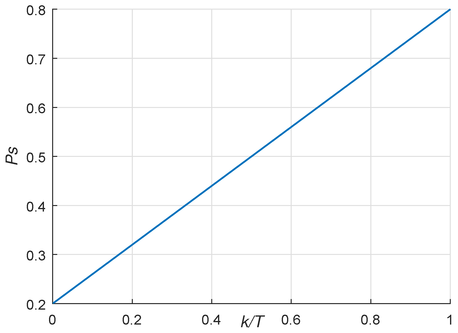
We designed 3 groups of experiments where $P_s$ either varies nonlinearly with the number of iterations, or varies linearly with the number of iterations, or is simply fixed. The nonlinear variation rule is shown in Equation (14) and Figure 4, and the linear variation rule is shown in Equation (26) and Figure 5:

$$\begin{array}{c}{P}_s=P_{s_{min}}+(P_{s_{max}}-P_{s_{min}})\times \frac{k}{T}\hfill \end{array}$$

(26)

where $P_{s_{min}}=0.2$ and $P_{s_{max}}=0.8$ are the same as in Equation (14) and in the fixed case $P_s$ is set to $0.5$. The complete experiment results are listed in

Table 9. $GD$ result of the local-global update probability $P_s$ of MOFECO algorithms on test functions. (The best result is bolded for each function).

Functions	${\mathit{P}}_{\mathit{s}}$ Is Nonlinear Variation	${\mathit{P}}_{\mathit{s}}$ Is Linear Variation	${\mathit{P}}_{\mathit{s}}=0.5$
ZDT1	$\mathbf{1.40}\mathbf{\times }{\mathbf{10}}^{\mathbf{-}\mathbf{4}}$	$1.72\times {10}^{-4}$	$1.54\times {10}^{-4}$
ZDT2	$4.02\times {10}^{-6}$	$4.05\times {10}^{-6}$	$\mathbf{3.67}\mathbf{\times }{\mathbf{10}}^{\mathbf{-}\mathbf{6}}$
ZDT4	$\mathbf{2.39}\mathbf{\times }{\mathbf{10}}^{\mathbf{-}\mathbf{5}}$	$2.70\times {10}^{-3}$	$5.78\times {10}^{-5}$
ZDT6	$\mathbf{3.50}\mathbf{\times }{\mathbf{10}}^{\mathbf{-}\mathbf{7}}$	$3.56\times {10}^{-7}$	$3.53\times {10}^{-7}$
DTLZ2	$\mathbf{7.43}\mathbf{\times }{\mathbf{10}}^{\mathbf{-}\mathbf{4}}$	$1.40\times {10}^{-3}$	$1.20\times {10}^{-3}$
DTLZ4	$1.43\times {10}^{-3}$	$\mathbf{2.86}\mathbf{\times }{\mathbf{10}}^{\mathbf{-}\mathbf{4}}$	$3.87\times {10}^{-4}$
DTLZ5	$3.56\times {10}^{-5}$	$1.18\times {10}^{-2}$	$\mathbf{2.18}\mathbf{\times }{\mathbf{10}}^{\mathbf{-}\mathbf{5}}$
DTLZ6	$\mathbf{4.82}\mathbf{\times }{\mathbf{10}}^{\mathbf{-}\mathbf{7}}$	$2.60\times {10}^{-6}$	$1.73\times {10}^{-6}$
DTLZ7	$\mathbf{9.60}\mathbf{\times }{\mathbf{10}}^{\mathbf{-}\mathbf{3}}$	$1.03\times {10}^{-2}$	$1.50\times {10}^{-2}$
WFG2	$\mathbf{6.25}\mathbf{\times }{\mathbf{10}}^{\mathbf{-}\mathbf{2}}$	$8.45\times {10}^{-2}$	$9.51\times {10}^{-2}$
WFG3	$\mathbf{5.29}\mathbf{\times }{\mathbf{10}}^{\mathbf{-}\mathbf{2}}$	$1.84\times {10}^{-1}$	$1.36\times {10}^{-1}$
WFG4	$\mathbf{1.57}\mathbf{\times }{\mathbf{10}}^{\mathbf{-}\mathbf{2}}$	$1.91\times {10}^{-2}$	$1.83\times {10}^{-2}$
MaF1	$\mathbf{7.10}\mathbf{\times }{\mathbf{10}}^{\mathbf{-}\mathbf{3}}$	$8.40\times {10}^{-3}$	$1.28\times {10}^{-2}$
MaF2	$3.67\times {10}^{-3}$	$5.30\times {10}^{-3}$	$\mathbf{2.60}\mathbf{\times }{\mathbf{10}}^{\mathbf{-}\mathbf{3}}$
MaF12	$1.88\times {10}^{-2}$	$2.00\times {10}^{-2}$	$\mathbf{1.81}\mathbf{\times }{\mathbf{10}}^{\mathbf{-}\mathbf{2}}$

,

Table 10. $IGD$ result of the local-global update probability $P_s$ of MOFECO algorithms on test functions. (The best result is bolded for each function).

Functions	${\mathit{P}}_{\mathit{s}}$ Is Nonlinear Variation	${\mathit{P}}_{\mathit{s}}$ Is Linear Variation	${\mathit{P}}_{\mathit{s}}=0.5$
ZDT1	$\mathbf{5.40}\mathbf{\times }{\mathbf{10}}^{\mathbf{-}\mathbf{3}}$	$5.50\times {10}^{-3}$	$5.60\times {10}^{-3}$
ZDT2	$\mathbf{5.40}\mathbf{\times }{\mathbf{10}}^{\mathbf{-}\mathbf{3}}$	$5.60\times {10}^{-3}$	$5.60\times {10}^{-3}$
ZDT4	$\mathbf{5.76}\mathbf{\times }{\mathbf{10}}^{\mathbf{-}\mathbf{3}}$	$3.01\times {10}^{-2}$	$5.80\times {10}^{-3}$
ZDT6	$4.70\times {10}^{-3}$	$4.60\times {10}^{-3}$	$\mathbf{4.30}\mathbf{\times }{\mathbf{10}}^{\mathbf{-}\mathbf{3}}$
DTLZ2	$7.49\times {10}^{-2}$	$7.66\times {10}^{-2}$	$\mathbf{7.10}\mathbf{\times }{\mathbf{10}}^{\mathbf{-}\mathbf{2}}$
DTLZ4	$\mathbf{1.21}\mathbf{\times }{\mathbf{10}}^{\mathbf{-}\mathbf{1}}$	$4.29\times {10}^{-1}$	$3.56\times {10}^{-1}$
DTLZ5	$\mathbf{6.70}\mathbf{\times }{\mathbf{10}}^{\mathbf{-}\mathbf{3}}$	$7.00\times {10}^{-3}$	$6.90\times {10}^{-3}$
DTLZ6	$\mathbf{6.40}\mathbf{\times }{\mathbf{10}}^{\mathbf{-}\mathbf{3}}$	$6.70\times {10}^{-3}$	$6.60\times {10}^{-3}$
DTLZ7	$\mathbf{2.88}\mathbf{\times }{\mathbf{10}}^{\mathbf{-}\mathbf{1}}$	$3.60\times {10}^{-1}$	$2.92\times {10}^{-1}$
WFG2	$\mathbf{5.11}\mathbf{\times }{\mathbf{10}}^{\mathbf{-}\mathbf{1}}$	$6.26\times {10}^{-1}$	$7.04\times {10}^{-1}$
WFG3	$\mathbf{1.60}\mathbf{\times }{\mathbf{10}}^{\mathbf{-}\mathbf{1}}$	$2.61\times {10}^{-1}$	$2.96\times {10}^{-1}$
WFG4	$7.89\times {10}^{-1}$	$7.86\times {10}^{-1}$	$\mathbf{7.74}\mathbf{\times }{\mathbf{10}}^{\mathbf{-}\mathbf{1}}$
MaF1	$\mathbf{1.21}\mathbf{\times }{\mathbf{10}}^{\mathbf{-}\mathbf{1}}$	$1.30\times {10}^{-1}$	$1.62\times {10}^{-1}$
MaF2	$9.58\times {10}^{-2}$	$9.49\times {10}^{-2}$	$\mathbf{8.34}\mathbf{\times }{\mathbf{10}}^{\mathbf{-}\mathbf{2}}$
MaF12	$\mathbf{7.43}\mathbf{\times }{\mathbf{10}}^{\mathbf{-}\mathbf{1}}$	$7.83\times {10}^{-1}$	$7.43\times {10}^{-1}$

and

Table 11. $SP$ result of the local-global update probability $P_s$ of MOFECO algorithms on test functions. (The best result is bolded for each function).

Functions	${\mathit{P}}_{\mathit{s}}$ Is Nonlinear Variation	${\mathit{P}}_{\mathit{s}}$ Is Linear Variation	${\mathit{P}}_{\mathit{s}}=0.5$
ZDT1	$\mathbf{8.70}\mathbf{\times }{\mathbf{10}}^{\mathbf{-}\mathbf{3}}$	$9.30\times {10}^{-3}$	$1.11\times {10}^{-2}$
ZDT2	$\mathbf{7.50}\mathbf{\times }{\mathbf{10}}^{\mathbf{-}\mathbf{3}}$	$7.50\times {10}^{-3}$	$7.90\times {10}^{-3}$
ZDT4	$\mathbf{7.40}\mathbf{\times }{\mathbf{10}}^{\mathbf{-}\mathbf{3}}$	$9.10\times {10}^{-3}$	$1.07\times {10}^{-2}$
ZDT6	$6.80\times {10}^{-3}$	$6.60\times {10}^{-3}$	$\mathbf{6.50}\mathbf{\times }{\mathbf{10}}^{\mathbf{-}\mathbf{3}}$
DTLZ2	$5.57\times {10}^{-2}$	$5.71\times {10}^{-2}$	$\mathbf{5.25}\mathbf{\times }{\mathbf{10}}^{\mathbf{-}\mathbf{2}}$
DTLZ4	$\mathbf{4.33}\mathbf{\times }{\mathbf{10}}^{\mathbf{-}\mathbf{2}}$	$5.74\times {10}^{-2}$	$4.88\times {10}^{-2}$
DTLZ5	$\mathbf{9.70}\mathbf{\times }{\mathbf{10}}^{\mathbf{-}\mathbf{3}}$	$1.04\times {10}^{-2}$	$1.01\times {10}^{-2}$
DTLZ6	$\mathbf{9.40}\mathbf{\times }{\mathbf{10}}^{\mathbf{-}\mathbf{3}}$	$9.60\times {10}^{-3}$	$9.50\times {10}^{-3}$
DTLZ7	$6.50\times {10}^{-2}$	$\mathbf{5.83}\mathbf{\times }{\mathbf{10}}^{\mathbf{-}\mathbf{2}}$	$8.18\times {10}^{-2}$
WFG2	$\mathbf{3.37}\mathbf{\times }{\mathbf{10}}^{\mathbf{-}\mathbf{1}}$	$3.94\times {10}^{-1}$	$4.06\times {10}^{-1}$
WFG3	$\mathbf{1.42}\mathbf{\times }{\mathbf{10}}^{\mathbf{-}\mathbf{1}}$	$2.92\times {10}^{-1}$	$2.05\times {10}^{-1}$
WFG4	$\mathbf{4.26}\mathbf{\times }{\mathbf{10}}^{\mathbf{-}\mathbf{1}}$	$4.88\times {10}^{-1}$	$4.54\times {10}^{-1}$
MaF1	$\mathbf{7.31}\mathbf{\times }{\mathbf{10}}^{\mathbf{-}\mathbf{2}}$	$8.14\times {10}^{-2}$	$5.71\times {10}^{-2}$
MaF12	$\mathbf{4.31}\mathbf{\times }{\mathbf{10}}^{\mathbf{-}\mathbf{1}}$	$4.67\times {10}^{-1}$	$4.42\times {10}^{-1}$

, which show average $GD$, $IGD$ and $SP$ values obtained by the above three case, and the bold part of the table represents the optimal values.

We can see from Table 9, Table 10 and Table 11 that when the local-global probability $P_s$ changes nonlinearly, the obtained Pareto solution set has smaller $GD$, $IGD$ and $SP$ values than the cases of linearly changing of $P_s$ and the fixed $P_s$. The advantage of choosing nonlinear variation $P_s$ lies in that it maintains a small value for a long time in the initial period of iteration, and a large value for a long time in the late iteration. Thereby increasing the global search time in the early stage of iteration and the local search time in the late stage of iteration can well balance the global and local search ability of MOFECO. Therefore, in the proposed algorithm, we choose a nonlinearly changing local-global probability $P_s$.

5.3.4. Comparison of Mutation Methods

The mutation operator has an important influence on the convergence and diversity of evolutionary algorithms. Based on the analysis of the mutation operator in Reference [25], it is found that the local search ability of Gaussian mutation is strong and the global search ability of uniform mutation is strong, while the local and global search capabilities of Cauchy mutation are centered. In this section, we choose two different mutation operators for comparative experiments and analysis. Method 1 combined Gaussian mutation, Uniform mutation and Cauchy mutation as mutation operator, which is shown in Equation (15); And method 2 uses only the Cauchy mutation, as shown in Equation (27), where the parameters $P_s$, ${\sigma }_1$, ${\sigma }_2$, ${\sigma }_3$ are set as Table 2. The comparative experiments results are shown in

Table 12. $GD$ result of the mutation methods of MOFECO algorithms on test functions. (The best result is bolded for each function).

Functions	Combined Mutation	Cauchy Mutation
ZDT1	$\mathbf{1.40}\mathbf{\times }{\mathbf{10}}^{\mathbf{-}\mathbf{4}}$	$1.50\times {10}^{-4}$
ZDT2	$4.02\times {10}^{-6}$	$\mathbf{2.46}\mathbf{\times }{\mathbf{10}}^{\mathbf{-}\mathbf{6}}$
ZDT4	$\mathbf{2.39}\mathbf{\times }{\mathbf{10}}^{\mathbf{-}\mathbf{5}}$	$1.50\times {10}^{-3}$
ZDT6	$\mathbf{3.50}\mathbf{\times }{\mathbf{10}}^{\mathbf{-}\mathbf{7}}$	$1.80\times {10}^{-3}$
DTLZ2	$\mathbf{7.43}\mathbf{\times }{\mathbf{10}}^{\mathbf{-}\mathbf{4}}$	$1.10\times {10}^{-3}$
DTLZ4	$1.43\times {10}^{-3}$	$\mathbf{7.65}\mathbf{\times }{\mathbf{10}}^{\mathbf{-}\mathbf{4}}$
DTLZ5	$3.56\times {10}^{-5}$	$\mathbf{3.36}\times {\mathbf{10}}^{-\mathbf{5}}$
DTLZ6	$\mathbf{4.82}\mathbf{\times }{\mathbf{10}}^{\mathbf{-}\mathbf{7}}$	$4.89\times {10}^{-7}$
DTLZ7	$9.60\times {10}^{-3}$	$\mathbf{7.30}\mathbf{\times }{\mathbf{10}}^{\mathbf{-}\mathbf{3}}$
WFG2	$\mathbf{6.25}\mathbf{\times }{\mathbf{10}}^{\mathbf{-}\mathbf{2}}$	$7.82\times {10}^{-2}$
WFG3	$\mathbf{5.29}\mathbf{\times }{\mathbf{10}}^{\mathbf{-}\mathbf{2}}$	$1.87\times {10}^{-1}$
WFG4	$\mathbf{1.57}\mathbf{\times }{\mathbf{10}}^{\mathbf{-}\mathbf{2}}$	$2.03\times {10}^{-2}$
MaF1	$\mathbf{7.10}\mathbf{\times }{\mathbf{10}}^{\mathbf{-}\mathbf{3}}$	$7.40\times {10}^{-3}$
MaF2	$3.67\times {10}^{-3}$	$\mathbf{2.60}\mathbf{\times }{\mathbf{10}}^{\mathbf{-}\mathbf{3}}$
MaF12	$\mathbf{1.88}\mathbf{\times }{\mathbf{10}}^{\mathbf{-}\mathbf{2}}$	$2.01\times {10}^{-2}$

,

Table 13. $IGD$ result of the mutation methods of MOFECO algorithms on test functions. (The best result is bolded for each function).

Functions	Combined Mutation	Cauchy Mutation
ZDT1	$\mathbf{5.40}\mathbf{\times }{\mathbf{10}}^{\mathbf{-}\mathbf{3}}$	$5.60\times {10}^{-3}$
ZDT2	$\mathbf{5.40}\mathbf{\times }{\mathbf{10}}^{\mathbf{-}\mathbf{3}}$	$6.40\times {10}^{-3}$
ZDT4	$\mathbf{5.76}\mathbf{\times }{\mathbf{10}}^{\mathbf{-}\mathbf{3}}$	$1.80\times {10}^{-2}$
ZDT6	$4.70\times {10}^{-3}$	$\mathbf{4.60}\mathbf{\times }{\mathbf{10}}^{\mathbf{-}\mathbf{3}}$
DTLZ2	$\mathbf{7.49}\mathbf{\times }{\mathbf{10}}^{\mathbf{-}\mathbf{2}}$	$7.54\times {10}^{-2}$
DTLZ4	$\mathbf{1.21}\mathbf{\times }{\mathbf{10}}^{\mathbf{-}\mathbf{1}}$	$3.83\times {10}^{-1}$
DTLZ5	$\mathbf{6.70}\mathbf{\times }{\mathbf{10}}^{\mathbf{-}\mathbf{3}}$	$7.00\times {10}^{-3}$
DTLZ6	$\mathbf{6.40}\mathbf{\times }{\mathbf{10}}^{\mathbf{-}\mathbf{3}}$	$6.60\times {10}^{-3}$
DTLZ7	$\mathbf{2.88}\mathbf{\times }{\mathbf{10}}^{\mathbf{-}\mathbf{1}}$	$4.30\times {10}^{-1}$
WFG2	$5.11\times {10}^{-1}$	$\mathbf{4.95}\mathbf{\times }{\mathbf{10}}^{\mathbf{-}\mathbf{1}}$
WFG3	$\mathbf{1.60}\mathbf{\times }{\mathbf{10}}^{\mathbf{-}\mathbf{1}}$	$3.01\times {10}^{-1}$
WFG4	$\mathbf{7.89}\mathbf{\times }{\mathbf{10}}^{\mathbf{-}\mathbf{1}}$	$7.97\times {10}^{-1}$
MaF1	$\mathbf{1.21}\mathbf{\times }{\mathbf{10}}^{\mathbf{-}\mathbf{1}}$	$1.21\times {10}^{-1}$
MaF2	$9.58\times {10}^{-2}$	$\mathbf{8.34}\mathbf{\times }{\mathbf{10}}^{\mathbf{-}\mathbf{2}}$
MaF12	$\mathbf{7.43}\mathbf{\times }{\mathbf{10}}^{\mathbf{-}\mathbf{1}}$	$7.63\times {10}^{-1}$

and

Table 14. $SP$ results of the mutation methods of MOFECO algorithms on test functions. (The best result is bolded for each function).

Functions	Combined Mutation	Cauchy Mutation
ZDT1	$\mathbf{8.70}\mathbf{\times }{\mathbf{10}}^{\mathbf{-}\mathbf{3}}$	$9.10\times {10}^{-3}$
ZDT2	$\mathbf{7.50}\mathbf{\times }{\mathbf{10}}^{\mathbf{-}\mathbf{3}}$	$8.10\times {10}^{-3}$
ZDT4	$\mathbf{7.40}\mathbf{\times }{\mathbf{10}}^{\mathbf{-}\mathbf{3}}$	$8.80\times {10}^{-3}$
ZDT6	$\mathbf{6.80}\mathbf{\times }{\mathbf{10}}^{\mathbf{-}\mathbf{3}}$	$1.74\times {10}^{-2}$
DTLZ2	$\mathbf{5.57}\mathbf{\times }{\mathbf{10}}^{\mathbf{-}\mathbf{2}}$	$5.63\times {10}^{-2}$
DTLZ4	$4.33\times {10}^{-2}$	$\mathbf{3.76}\mathbf{\times }{\mathbf{10}}^{\mathbf{-}\mathbf{2}}$
DTLZ5	$\mathbf{9.70}\mathbf{\times }{\mathbf{10}}^{\mathbf{-}\mathbf{3}}$	$1.13\times {10}^{-2}$
DTLZ6	$\mathbf{9.40}\mathbf{\times }{\mathbf{10}}^{\mathbf{-}\mathbf{3}}$	$9.60\times {10}^{-3}$
DTLZ7	$6.50\times {10}^{-2}$	$\mathbf{5.34}\mathbf{\times }{\mathbf{10}}^{\mathbf{-}\mathbf{2}}$
WFG2	$\mathbf{3.37}\mathbf{\times }{\mathbf{10}}^{\mathbf{-}\mathbf{1}}$	$4.33\times {10}^{-1}$
WFG3	$\mathbf{1.42}\mathbf{\times }{\mathbf{10}}^{\mathbf{-}\mathbf{1}}$	$3.02\times {10}^{-1}$
WFG4	$\mathbf{4.26}\mathbf{\times }{\mathbf{10}}^{\mathbf{-}\mathbf{1}}$	$4.84\times {10}^{-1}$
MaF1	$\mathbf{7.31}\mathbf{\times }{\mathbf{10}}^{\mathbf{-}\mathbf{2}}$	$8.42\times {10}^{-2}$
MaF2	$6.27\times {10}^{-2}$	$\mathbf{5.71}\mathbf{\times }{\mathbf{10}}^{\mathbf{-}\mathbf{2}}$
MaF12	$\mathbf{4.31}\mathbf{\times }{\mathbf{10}}^{\mathbf{-}\mathbf{1}}$	$4.52\times {10}^{-1}$

, which give average $GD$, $IGD$ and $SP$ values obtained by the above two mutation operators and the bold part of the table represents the optimal values.

$$\begin{array}{c}X{M}_{ij}(k+1)=X{C}_{ij}(k+1)+C(0,{\sigma }_2)\hfill \end{array}$$

(27)

From the experimental results of Table 12, Table 13 and Table 14, we can see that the Pareto solution set obtained by MOFECO using combinatorial mutation has smaller $GD$, $IGD$ and $SP$ values than with using only Cauchy mutation. The reason may be that combinatorial optimization takes full account of the characteristics of Pre-iteration and late iteration, which can better adapt to the changes in the population. Thence, we choose the combined mutation in MOFECO.

In summary, through the above experiment, the MOFECO parameters are configured as follows. Equation (11) is adopted for the update condition, the variation of local-global update probability $P_s$ is nonlinear, and the mutation operator uses the combined mutation method.

5.4. Comparison with Other Optimization Algorithms

In this section, the performances of MOFECO were verified by empirically comparing it with three classic MOEAs NSGA-II [5], MOPSO [12], PESA-II [11], and two latest algorithms KnEA [2] and NSLS [15]. For a fair-minded comparison, we adopt the consistent parameters of population size $N=100$ and termination condition $T=1000$ for all the six algorithms. The other parameters of MOFECO are shown in Table 2. For the other parameters used in NSGA-II, MOPSO, PESA-II, KnEA and NSLS, they are consistent with the parameters in their original study [2,5,11,12,15]. The detailed parameters configuration for the five compared algorithms are shown in

Table 15. The detailed parameter configuration for the five compared algorithms.

Algorithms	EAreal						PSO	NSLS Operator
	$\mathit{proC}$	$\mathit{proM}$	$\mathit{disC}$	$\mathit{disM}$	$\mathit{div}$	$\mathit{rate}$	$\mathit{\omega }$	$\mathit{mu}$	$\mathit{delta}$
NSGA-II	1	1	20	20	/	/	/	/	/
PESA-II	1	1	20	20	10	/	/	/	/
KnEA	1	1	20	20	/	0.4	/	/	/
MOPSO	/	/	/	/	/	/	0.4	/	/
NSLS	/	/	/	/	/	/	/	0.5	0.1

.

In the EAreal operator, $proC$ is the probability of implementing crossover operation, $proM$ is the expectation of polynomial mutation, $disC$ represents the distribution index of simulated binary crossover, and $disM$ represent the distribution index of polynomial mutation. In PESA-II, $div$ is the number of divisions in each objective. In KnEA, $rate$ represents the rate of knee points in the population. In MOPSO, $\omega$ represents the weight factor, and in the NSLS operator, the $mu$ is the mean value of the Gaussian distribution and $delta$ is the standard deviation of the Gaussian distribution.

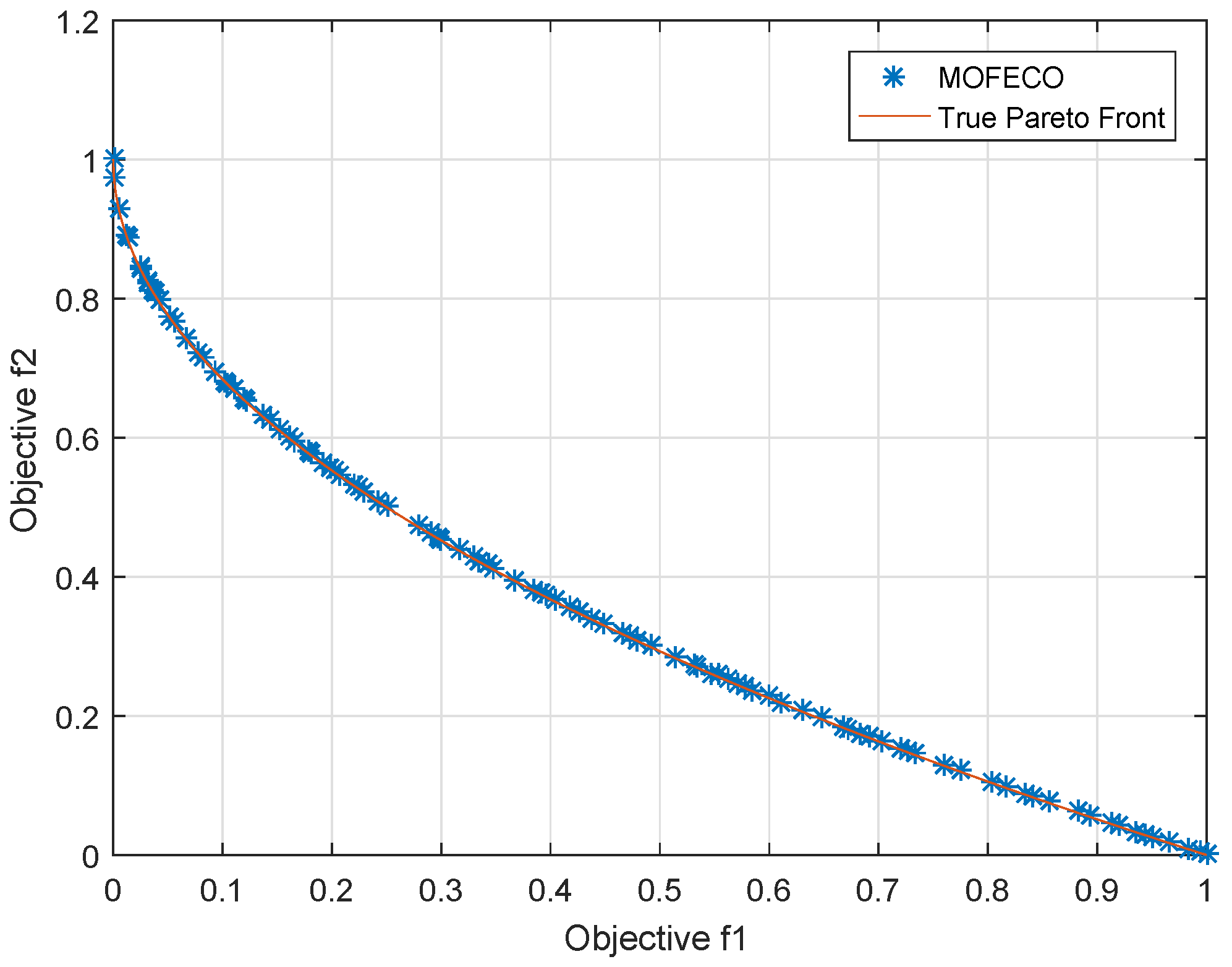
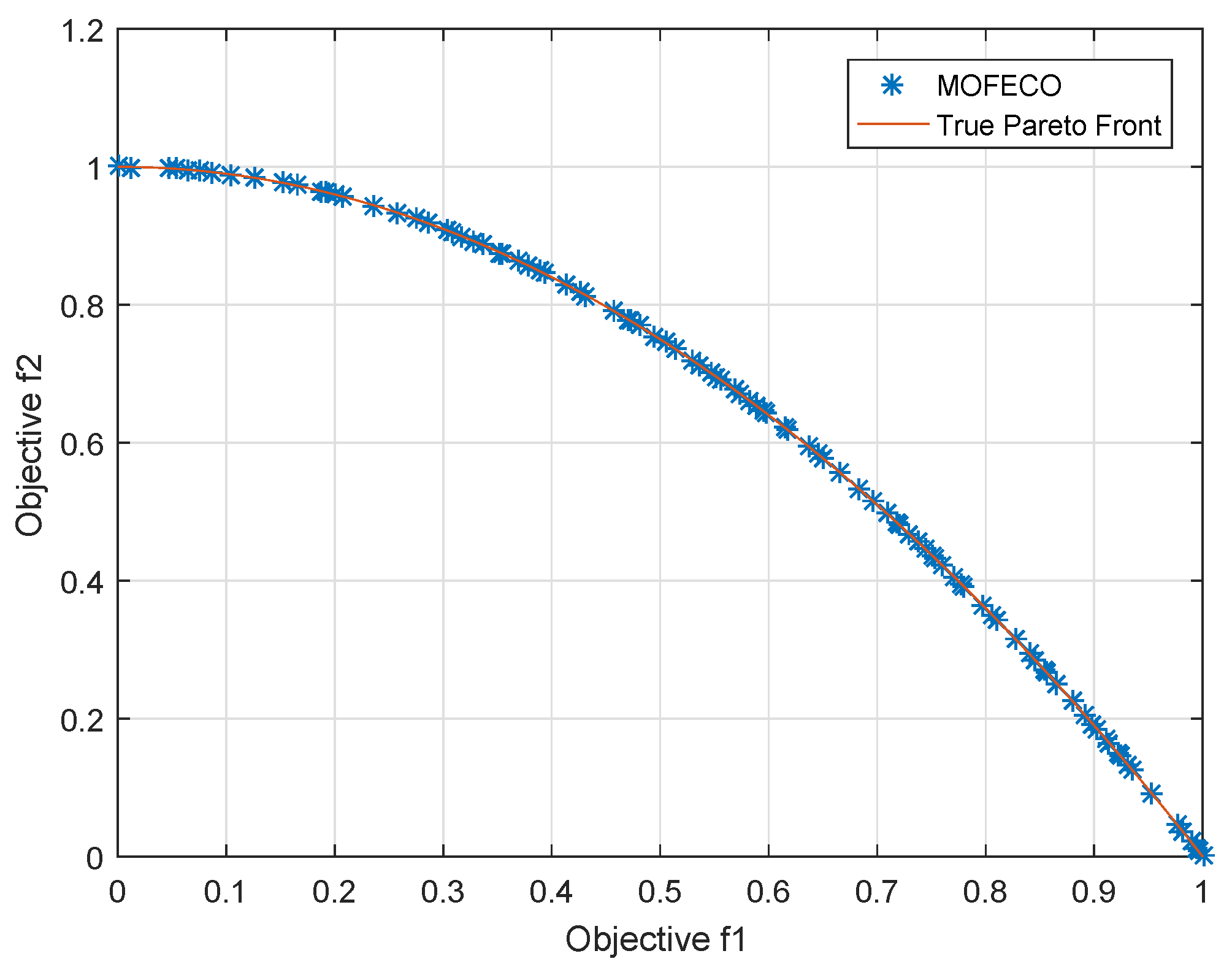
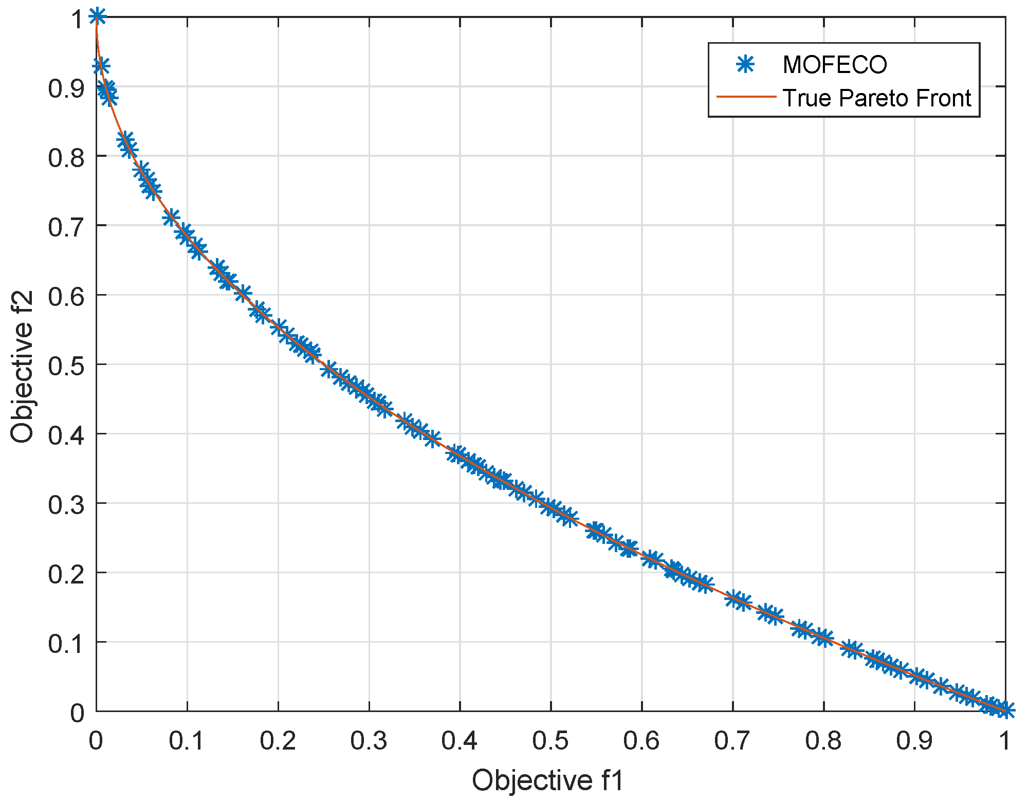
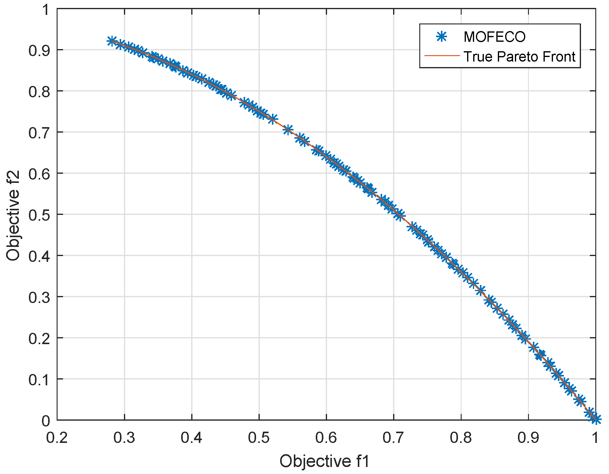
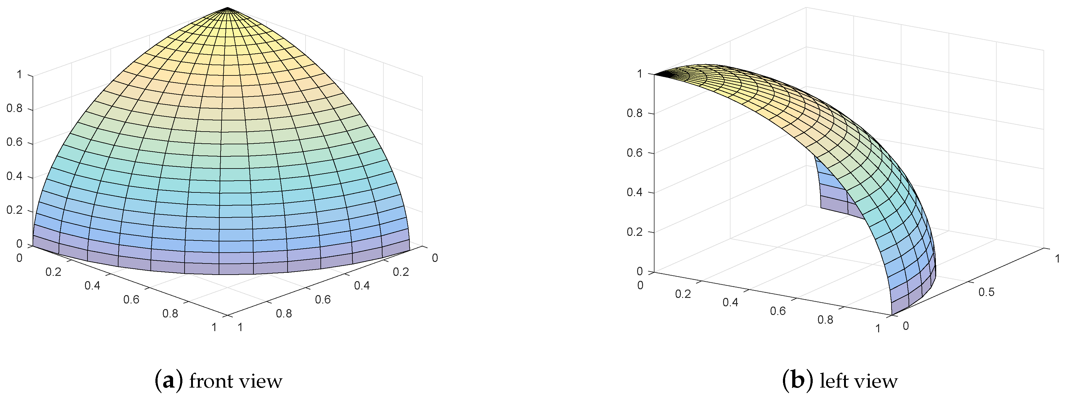
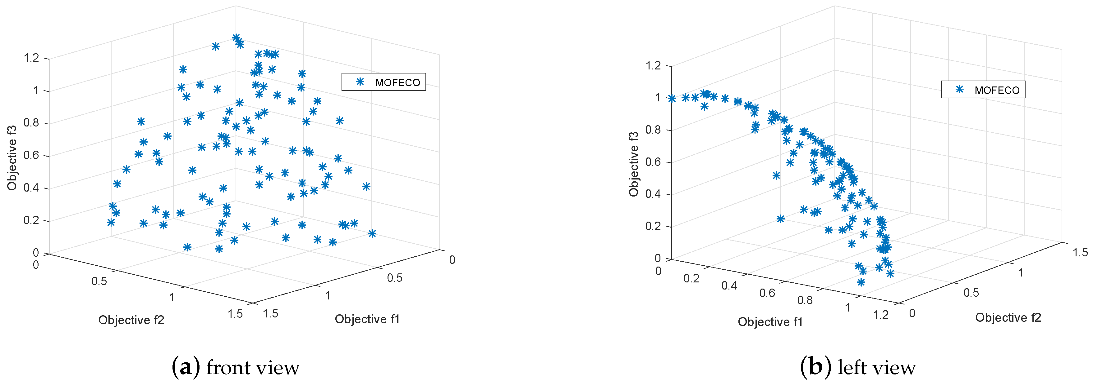
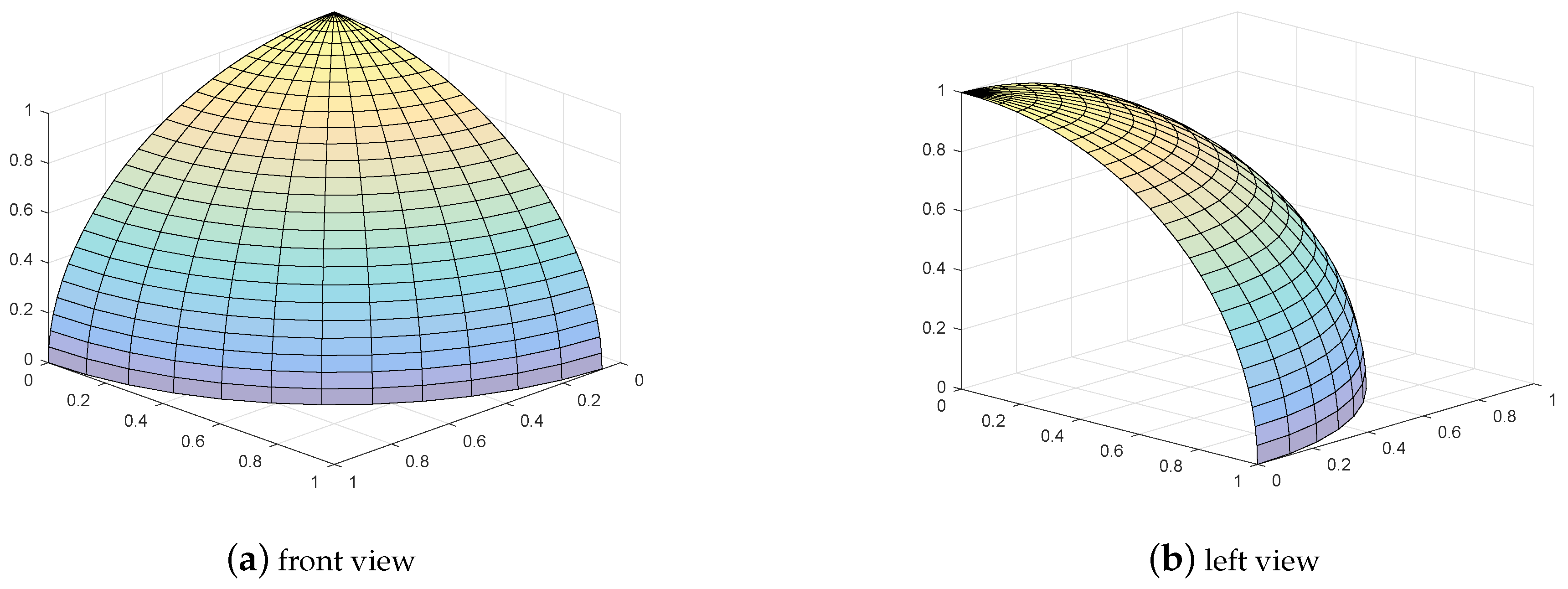
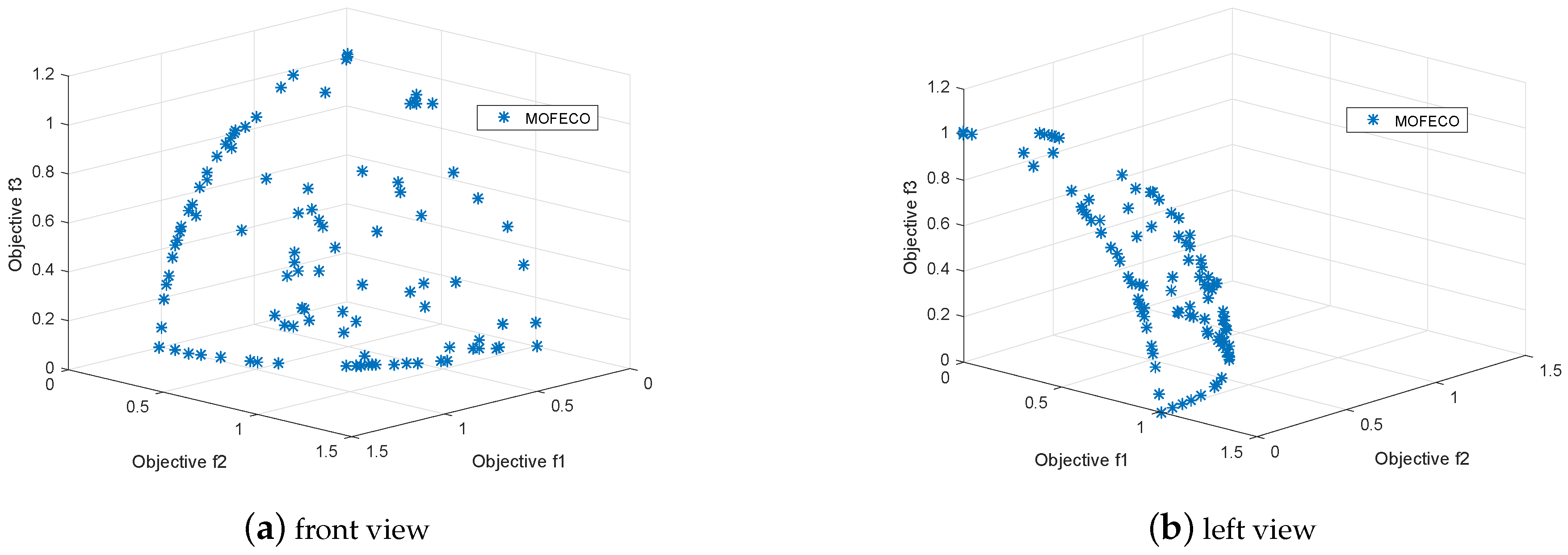
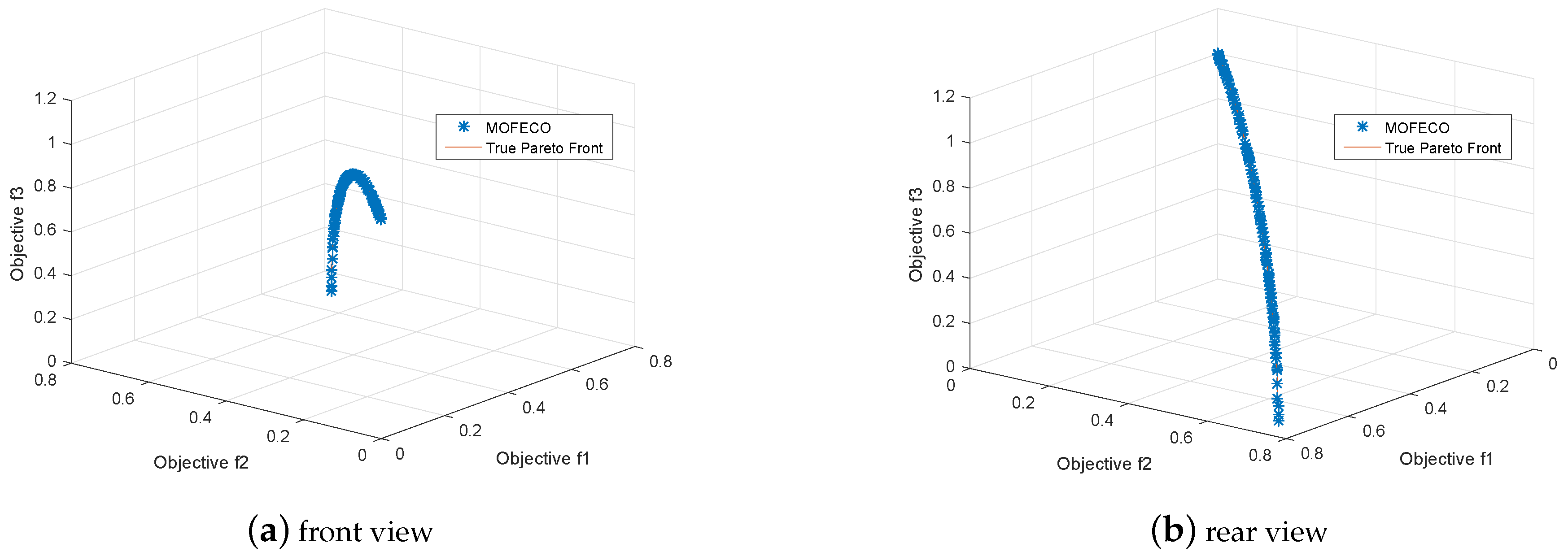
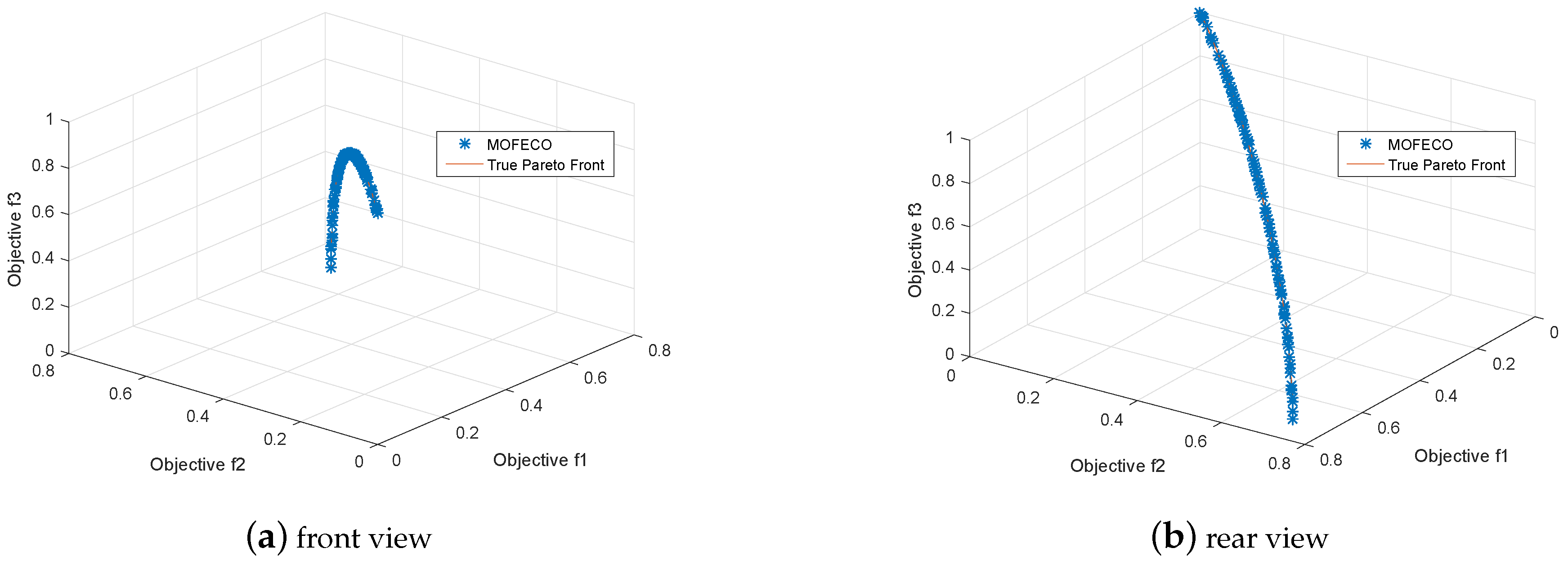
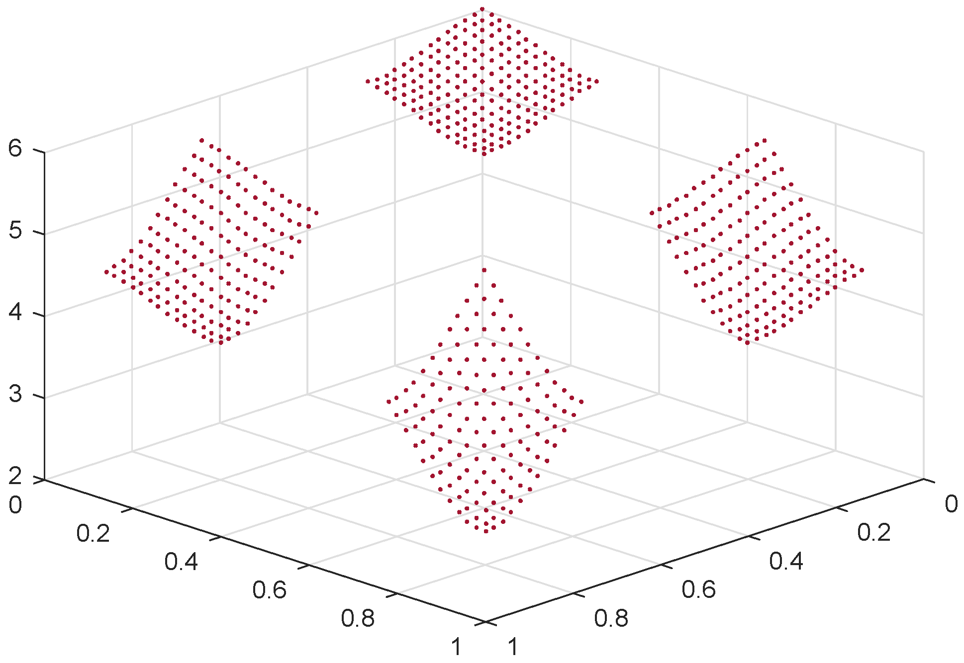
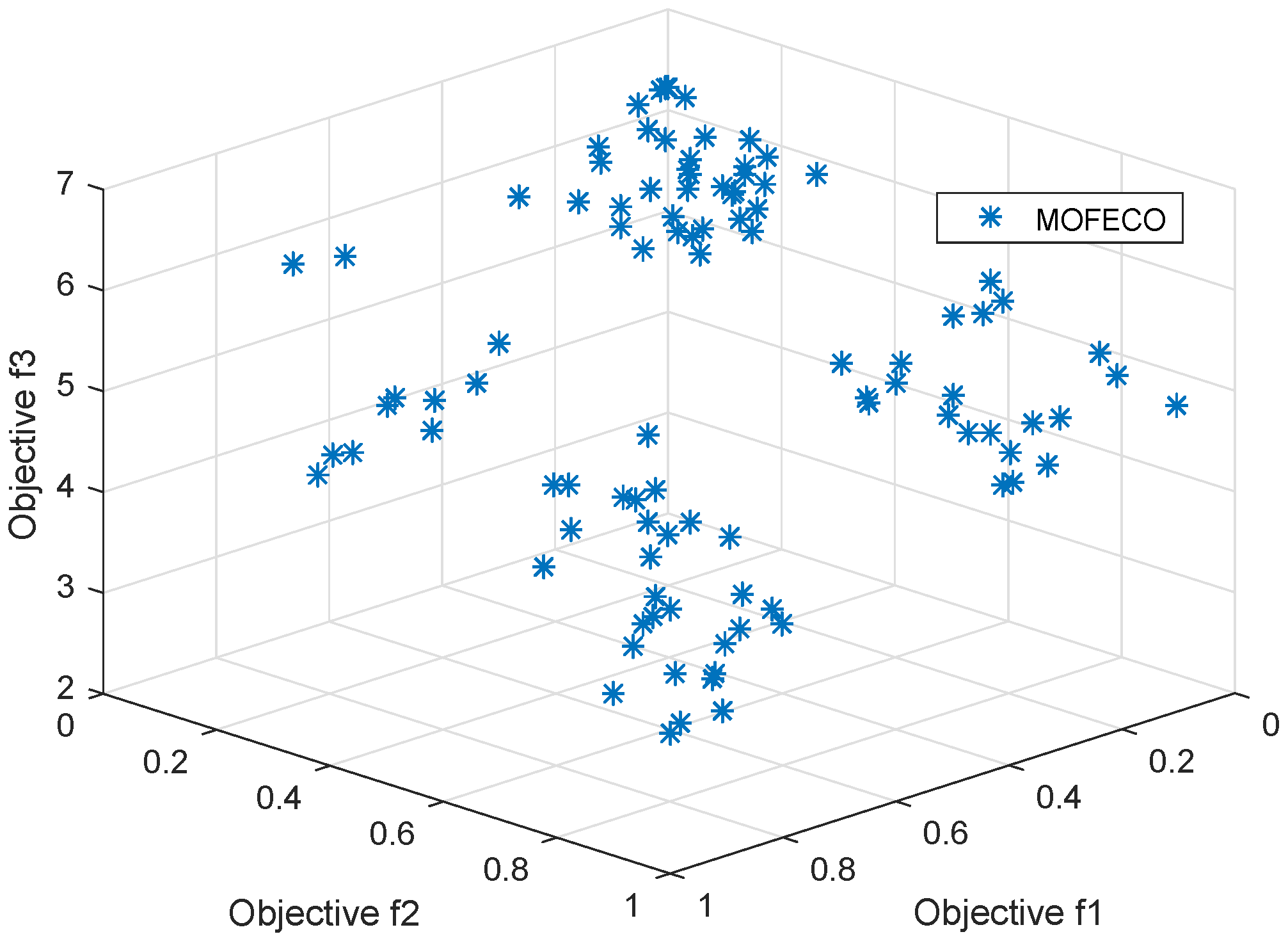
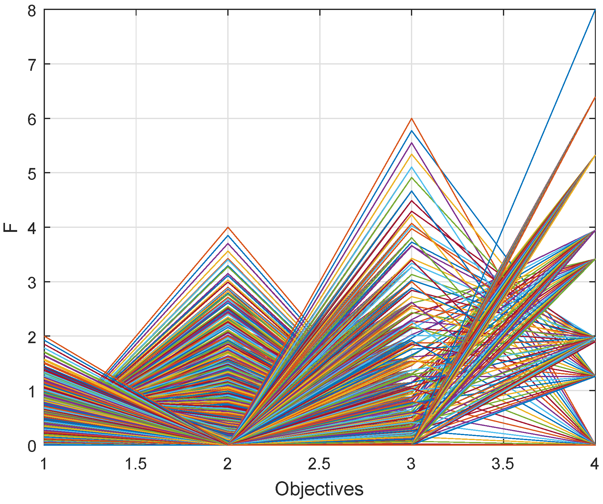
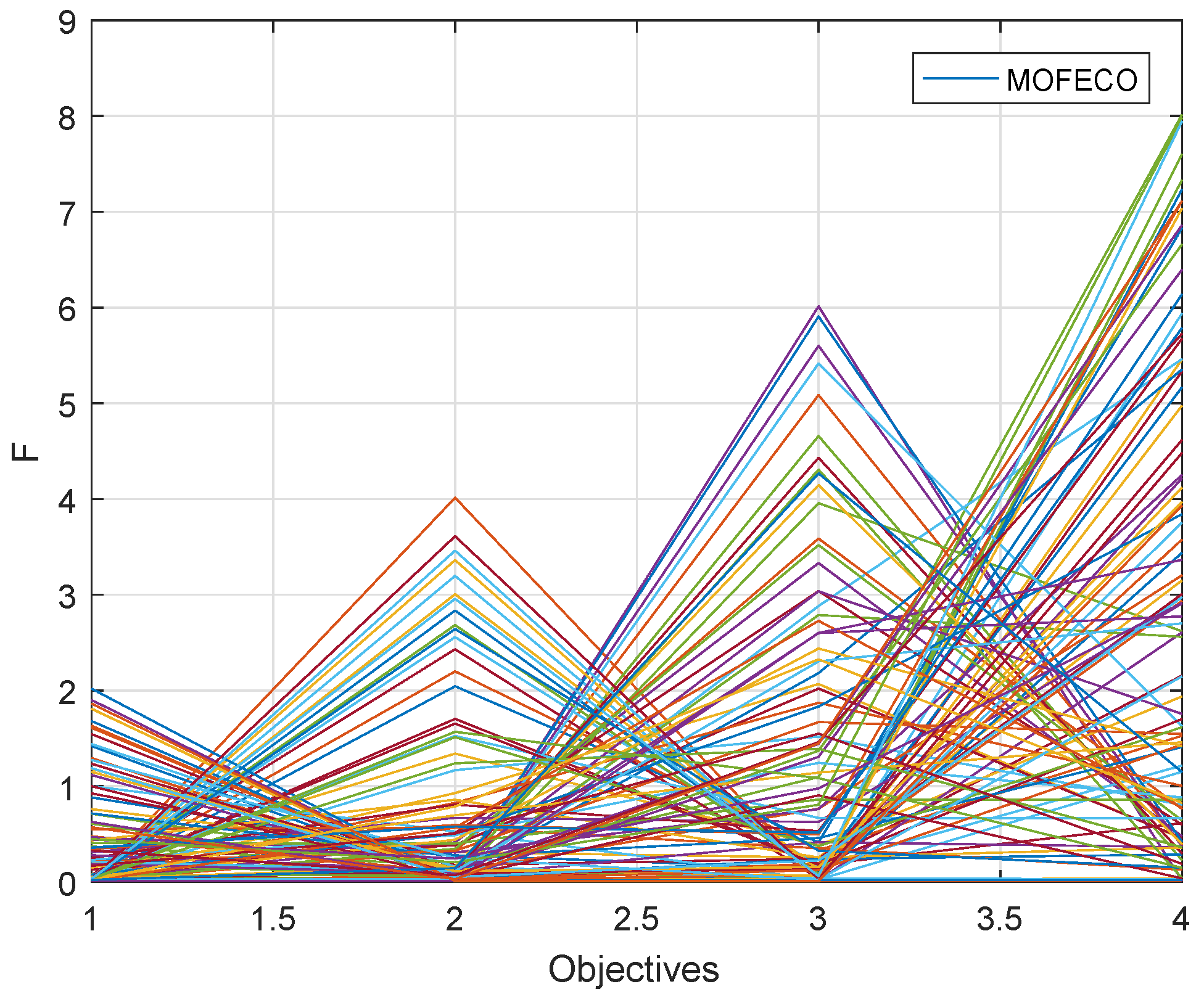
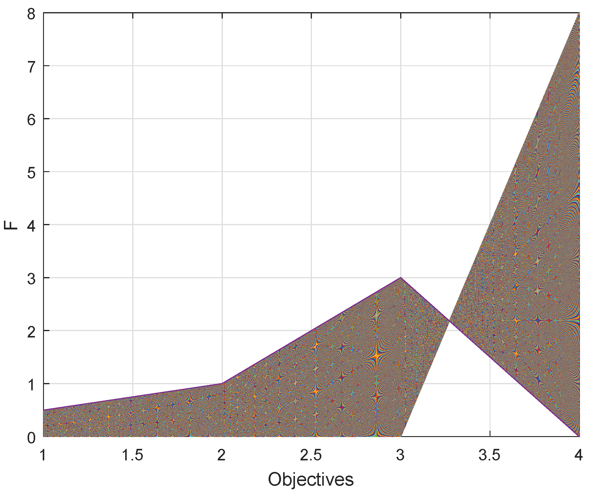
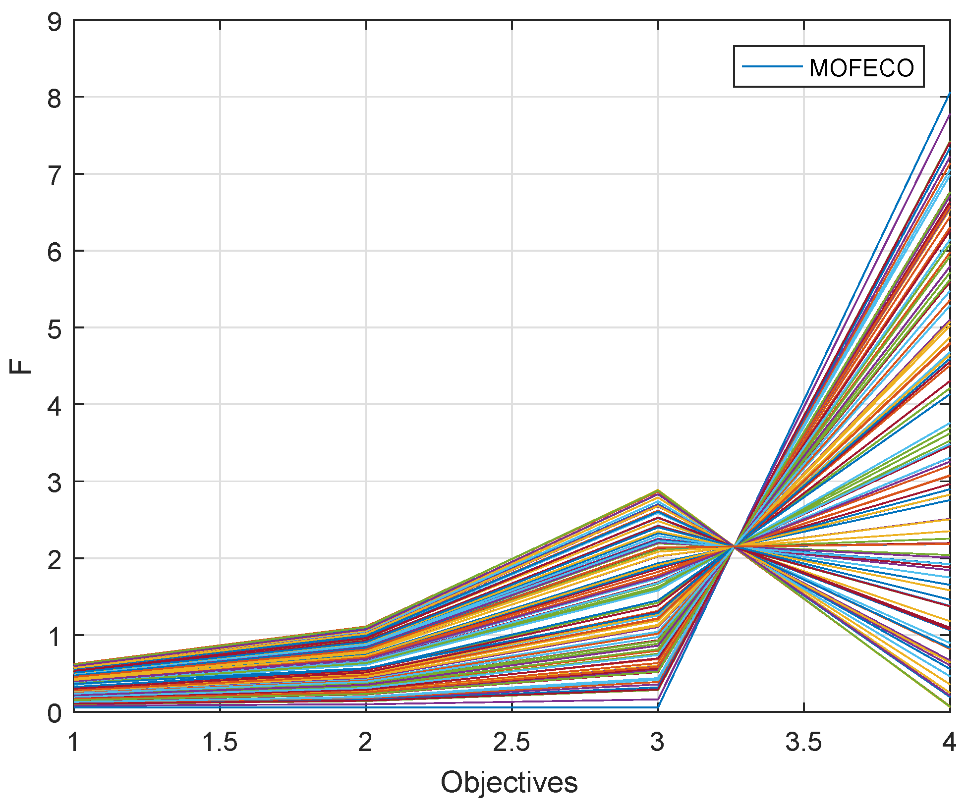
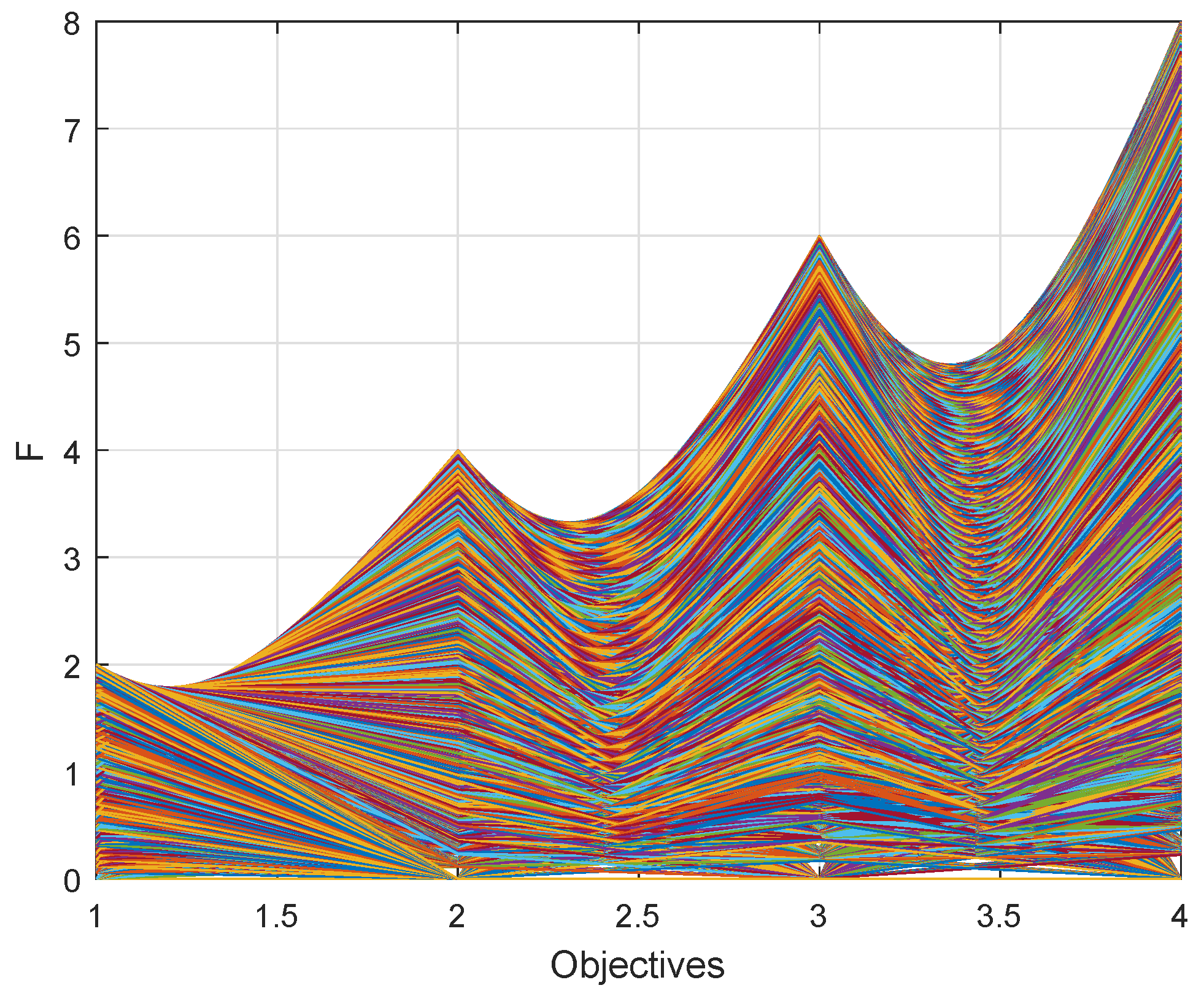
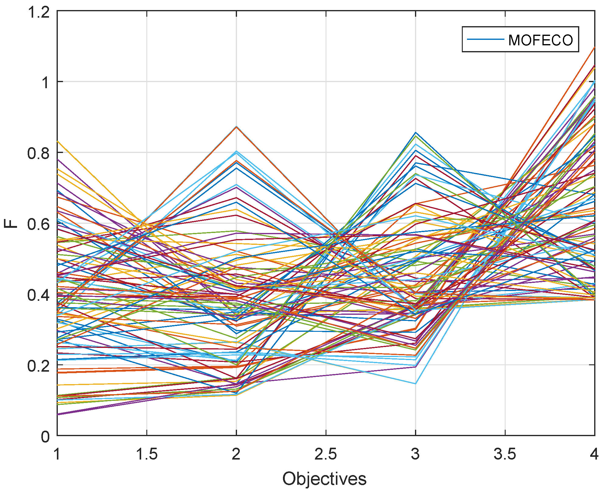
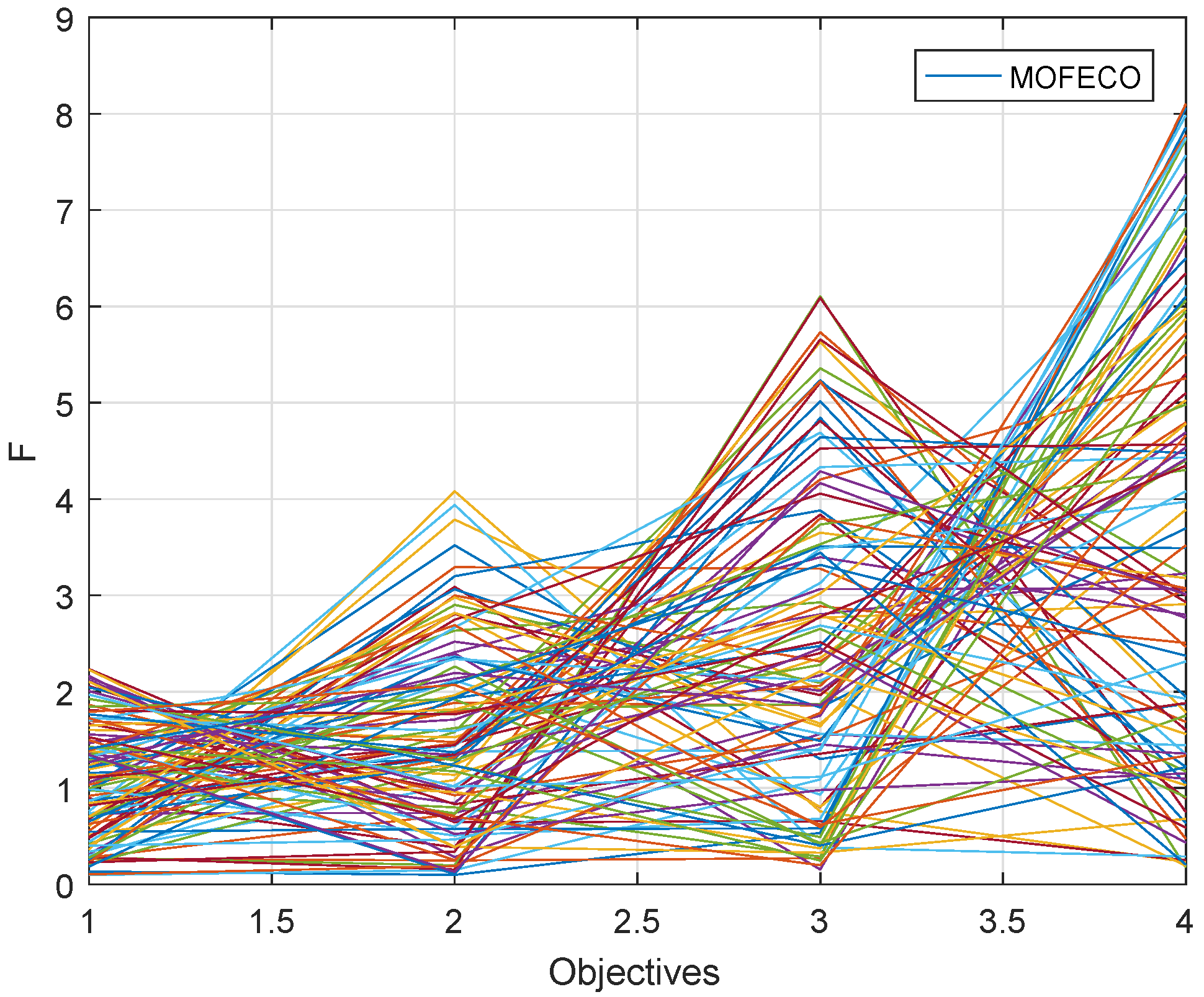
We use the proposed MOFECO algorithm to optimize 15 test functions selected from the ZDT, DTLZ, MaF and WFG series in the aforementioned environment, and the obtained Pareto front by MOFECO and the true Pareto front are shown in Figure 6, Figure 7, Figure 8, Figure 9, Figure 10, Figure 11, Figure 12, Figure 13, Figure 14, Figure 15, Figure 16, Figure 17, Figure 18, Figure 19, Figure 20, Figure 21, Figure 22, Figure 23, Figure 24, Figure 25, Figure 26, Figure 27, Figure 28 and Figure 29. Figure 10 and Figure 12 shows the true Pareto front of the test function DTLZ2 and DTLZ4, and each of the plots from Figure 10, Figure 11, Figure 12, Figure 13, Figure 14 and Figure 15 has two subgraphs, respectively representing the front and left or rear view of the optimized Pareto front in problems DTLZ2, DTLZ4, DTLZ5 and DTLZ6.

From Figure 6, Figure 7, Figure 8, Figure 9, Figure 10, Figure 11, Figure 12, Figure 13, Figure 14, Figure 15, Figure 16, Figure 17, Figure 18, Figure 19, Figure 20, Figure 21, Figure 22, Figure 23, Figure 24, Figure 25, Figure 26, Figure 27, Figure 28 and Figure 29, we can see that the obtained Pareto front by using the proposed MOFECO can evenly distribute on the true Pareto front, which shows that the algorithm can converge to the optimal solution set and is effective in solving MOO problems.

For quantitative analysis,

Table 16. $GD$ result of the six compared algorithms on test functions. (“+”, “∼” and “-” respectively represent that MOFECO is better than, similar to and inferior to the other five algorithms).

Problems	MOFECO	NSGA-II	MOPSO	PESA-II	KnEA	NSLS
ZDT1	$1.40\times {10}^{-4}$	$1.54\times {10}^{-4}$ (+)	$6.94\times {10}^{-4}$ (+)	$1.72\times {10}^{-4}$ (+)	$5.36\times {10}^{-5}$ (-)	$5.04\times {10}^{-4}$ (+)
ZDT2	$4.02\times {10}^{-6}$	$2.36\times {10}^{-5}$ (+)	$2.00\times {10}^{-3}$ (+)	$5.75\times {10}^{-4}$ (+)	$5.59\times {10}^{-6}$ (+)	$3.80\times {10}^{-3}$ (+)
ZDT4	$2.39\times {10}^{-5}$	$2.81\times {10}^{-5}$ (+)	$9.30\times {10}^{-3}$ (+)	$2.09\times {10}^{-2}$ (+)	$1.42\times {10}^{-2}$ (+)	$1.81\times {10}^{-2}$ (+)
ZDT6	$3.50\times {10}^{-7}$	$4.02\times {10}^{-6}$ (+)	$9.13\times {10}^{-2}$ (+)	$6.10\times {10}^{-3}$ (+)	$4.36\times {10}^{-6}$ (+)	$7.30\times {10}^{-3}$ (+)
DTLZ2	$4.67\times {10}^{-4}$	$1.20\times {10}^{-3}$ (+)	$4.70\times {10}^{-3}$ (+)	$1.40\times {10}^{-3}$ (+)	$5.03\times {10}^{-4}$ (+)	$5.56\times {10}^{-4}$ (+)
DTLZ4	$1.43\times {10}^{-3}$	$1.10\times {10}^{-3}$ (-)	$4.60\times {10}^{-3}$ (+)	$1.42\times {10}^{-3}$ (∼)	$4.24\times {10}^{-4}$ (-)	$6.05\times {10}^{-4}$ (-)
DTLZ5	$3.56\times {10}^{-5}$	$2.30\times {10}^{-4}$ (+)	$1.40\times {10}^{-3}$ (+)	$2.19\times {10}^{-4}$ (+)	$5.00\times {10}^{-4}$ (+)	$1.46\times {10}^{-5}$ (-)
DTLZ6	$4.82\times {10}^{-7}$	$4.82\times {10}^{-6}$ (+)	$5.20\times {10}^{-3}$ (+)	$1.80\times {10}^{-3}$ (+)	$4.73\times {10}^{-6}$ (+)	$4.85\times {10}^{-6}$ (+)
DTLZ7	$9.60\times {10}^{-3}$	$3.00\times {10}^{-3}$ (-)	$1.01\times {10}^{-2}$ (+)	$2.70\times {10}^{-3}$ (-)	$1.50\times {10}^{-3}$ (-)	$2.90\times {10}^{-3}$ (-)
WFG2	$6.25\times {10}^{-2}$	$8.77\times {10}^{-2}$ (+)	$7.12\times {10}^{-2}$ (+)	$6.44\times {10}^{-2}$ (+)	$6.51\times {10}^{-2}$ (+)	$6.66\times {10}^{-2}$ (+)
WFG3	$5.29\times {10}^{-2}$	$1.85\times {10}^{-1}$ (+)	$1.46\times {10}^{-1}$ (+)	$1.63\times {10}^{-1}$ (+)	$1.21\times {10}^{-1}$ (+)	$1.62\times {10}^{-1}$ (+)
WFG4	$1.57\times {10}^{-2}$	$1.68\times {10}^{-2}$ (+)	$3.61\times {10}^{-2}$ (+)	$2.58\times {10}^{-2}$ (+)	$1.59\times {10}^{-2}$ (∼)	$4.39\times {10}^{-2}$ (+)
MaF1	$7.10\times {10}^{-3}$	$3.97\times {10}^{-3}$ (-)	$9.72\times {10}^{-3}$ (+)	$4.29\times {10}^{-3}$ (-)	$1.75\times {10}^{-3}$ (-)	$6.14\times {10}^{-3}$ (-)
MaF2	$3.67\times {10}^{-3}$	$8.13\times {10}^{-3}$ (+)	$4.88\times {10}^{-3}$ (+)	$3.79\times {10}^{-3}$ (+)	$4.35\times {10}^{-3}$ (+)	$6.19\times {10}^{-3}$ (+)
MaF12	$1.88\times {10}^{-2}$	$2.01\times {10}^{-2}$ (+)	$4.11\times {10}^{-2}$ (+)	$2.20\times {10}^{-2}$ (+)	$2.01\times {10}^{-2}$ (+)	$5.83\times {10}^{-2}$ (+)
+	/	12	15	12	10	11
-	/	3	0	2	4	4
∼	/	0	0	1	1	0

,

Table 17. $PD$ result of the six compared algorithms on test functions. (“+”, “∼” and “-” respectively represent that MOFECO is better than, similar to and inferior to the other five algorithms).

Problems	MOFECO	NSGA-II	MOPSO	PESA-II	KnEA	NSLS
ZDT1	$1.73\times {10}^3$	$1.71\times {10}^3$ (+)	$1.47\times {10}^3$ (+)	$1.45\times {10}^3$ (+)	$1.06\times {10}^3$ (+)	$1.52\times {10}^3$ (+)
ZDT2	$1.74\times {10}^3$	$1.73\times {10}^3$ (∼)	$1.53\times {10}^3$ (+)	$1.44\times {10}^3$ (+)	$1.30\times {10}^3$ (+)	$1.36\times {10}^3$ (+)
ZDT4	$1.69\times {10}^3$	$1.63\times {10}^3$ (+)	$8.40\times {10}^2$ (+)	$1.57\times {10}^3$ (+)	$7.27\times {10}^2$ (+)	$1.98\times {10}^3$ (+)
ZDT6	$1.62\times {10}^3$	$1.45\times {10}^3$ (+)	$1.30\times {10}^3$ (+)	$1.27\times {10}^3$ (+)	$1.53\times {10}^3$ (+)	$1.35\times {10}^3$ (+)
DTLZ2	$1.73\times {10}^5$	$1.87\times {10}^5$ (-)	$1.99\times {10}^5$ (-)	$1.85\times {10}^5$ (-)	$1.00\times {10}^5$ (+)	$1.56\times {10}^5$ (+)
DTLZ4	$1.32\times {10}^5$	$1.88\times {10}^5$ (-)	$1.69\times {10}^5$ (-)	$1.70\times {10}^5$ (-)	$8.39\times {10}^4$ (+)	$8.41\times {10}^4$ (+)
DTLZ5	$7.30\times {10}^4$	$7.10\times {10}^4$ (+)	$7.27\times {10}^4$ (+)	$6.29\times {10}^4$ (+)	$7.36\times {10}^4$ (-)	$7.20\times {10}^4$ (+)
DTLZ6	$7.97\times {10}^4$	$7.20\times {10}^4$ (+)	$6.85\times {10}^4$ (+)	$6.66\times {10}^4$ (+)	$7.57\times {10}^4$ (+)	$6.94\times {10}^4$ (+)
DTLZ7	$1.42\times {10}^5$	$2.00\times {10}^5$ (-)	$1.72\times {10}^5$ (-)	$1.35\times {10}^5$ (+)	$1.42\times {10}^5$ (∼)	$1.75\times {10}^5$ (-)
WFG2	$9.78\times {10}^6$	$8.80\times {10}^6$ (+)	$9.78\times {10}^6$ (∼)	$9.55\times {10}^6$ (+)	$5.3\times {10}^6$ (+)	$8.57\times {10}^6$ (+)
WFG3	$8.38\times {10}^6$	$1.20\times {10}^7$ (-)	$8.17\times {10}^6$ (+)	$7.13\times {10}^6$ (+)	$1.02\times {10}^7$ (-)	$1.38\times {10}^7$ (-)
WFG4	$1.92\times {10}^7$	$1.90\times {10}^7$ (+)	$1.84\times {10}^7$ (+)	$1.68\times {10}^7$ (+)	$7.06\times {10}^6$ (+)	$1.69\times {10}^7$ (+)
MaF1	$3.54\times {10}^6$	$3.26\times {10}^6$ (+)	$3.49\times {10}^6$ (+)	$3.09\times {10}^6$ (+)	$2.74\times {10}^6$ (+)	$3.06\times {10}^6$ (+)
MaF2	$2.74\times {10}^6$	$2.57\times {10}^6$ (+)	$2.30\times {10}^6$ (+)	$2.14\times {10}^6$ (+)	$1.52\times {10}^6$ (+)	$2.67\times {10}^6$ (+)
MaF12	$1.96\times {10}^7$	$1.85\times {10}^7$ (+)	$1.90\times {10}^7$ (+)	$1.93\times {10}^7$ (+)	$9.25\times {10}^6$ (+)	$1.55\times {10}^7$ (+)
+	/	10	11	13	12	12
-	/	4	3	2	2	3
∼	/	1	1	0	1	0

,

Table 18. $HV$ result of the six compared algorithms on test functions. (“+”, “∼” and “-” respectively represent that MOFECO is better than, similar to and inferior to the other five algorithms).

Problems	MOFECO	NSGA-II	MOPSO	PESA-II	KnEA	NSLS
ZDT1	$8.70\times {10}^{-1}$	$8.70\times {10}^{-1}$ (∼)	$8.58\times {10}^{-1}$ (+)	$8.62\times {10}^{-1}$ (+)	$7.62\times {10}^{-1}$ (+)	$8.66\times {10}^{-1}$ (+)
ZDT2	$5.37\times {10}^{-1}$	$5.35\times {10}^{-1}$ (+)	$5.28\times {10}^{-1}$ (+)	$5.25\times {10}^{-1}$ (+)	$3.90\times {10}^{-1}$ (+)	$4.95\times {10}^{-1}$ (+)
ZDT4	$8.68\times {10}^{-1}$	$8.61\times {10}^{-1}$ (+)	$6.88\times {10}^{-1}$ (+)	$8.62\times {10}^{-1}$ (+)	$6.64\times {10}^{-1}$ (+)	$6.15\times {10}^{-1}$ (+)
ZDT6	$4.33\times {10}^{-1}$	$4.33\times {10}^{-1}$ (∼)	$3.95\times {10}^{-1}$ (+)	$4.28\times {10}^{-1}$ (+)	$4.30\times {10}^{-1}$ (+)	$4.33\times {10}^{-1}$ (∼)
DTLZ2	$6.70\times {10}^{-1}$	$7.08\times {10}^{-1}$ (-)	$6.61\times {10}^{-1}$ (+)	$6.94\times {10}^{-1}$ (-)	$7.21\times {10}^{-1}$ (-)	$7.46\times {10}^{-1}$ (-)
DTLZ4	$8.08\times {10}^{-1}$	$6.92\times {10}^{-1}$ (+)	$6.78\times {10}^{-1}$ (+)	$7.14\times {10}^{-1}$ (+)	$7.09\times {10}^{-1}$ (+)	$7.07\times {10}^{-1}$ (+)
DTLZ5	$1.33\times {10}^{-1}$	$1.33\times {10}^{-1}$ (∼)	$1.27\times {10}^{-1}$ (+)	$1.28\times {10}^{-1}$ (+)	$1.29\times {10}^{-1}$ (+)	$1.33\times {10}^{-1}$ (∼)
DTLZ6	$1.33\times {10}^{-1}$	$1.33\times {10}^{-1}$ (∼)	$1.30\times {10}^{-1}$ (+)	$1.27\times {10}^{-1}$ (+)	$1.33\times {10}^{-1}$ (∼)	$1.33\times {10}^{-1}$ (∼)
DTLZ7	$1.30\times {10}^0$	$1.58\times {10}^0$ (-)	$1.42\times {10}^0$ (-)	$1.53\times {10}^0$ (-)	$1.61\times {10}^0$ (-)	$1.62\times {10}^0$ (-)
WFG2	$5.47\times {10}^2$	$5.40\times {10}^2$ (+)	$4.73\times {10}^2$ (+)	$5.26\times {10}^2$ (+)	$5.41\times {10}^2$ (+)	$5.01\times {10}^2$ (+)
WFG3	$5.01\times {10}^0$	$5.19\times {10}^0$ (-)	$0.00\times {10}^0$ (+)	$0.00\times {10}^0$ (+)	$3.93\times {10}^0$ (+)	$1.81\times {10}^0$ (+)
WFG4	$3.25\times {10}^2$	$3.50\times {10}^2$ (-)	$2.43\times {10}^2$ (+)	$2.60\times {10}^2$ (+)	$3.71\times {10}^2$ (-)	$3.20\times {10}^2$ (+)
MaF1	$5.84\times {10}^{-2}$	$6.19\times {10}^{-2}$ (-)	$4.75\times {10}^{-2}$ (+)	$6.16\times {10}^{-2}$ (-)	$7.51\times {10}^{-2}$ (-)	$5.03\times {10}^{-2}$ (+)
MaF2	$1.37\times {10}^{-1}$	$1.32\times {10}^{-1}$ (+)	$1.18\times {10}^{-1}$ (+)	$1.15\times {10}^{-1}$ (+)	$1.33\times {10}^{-1}$ (+)	$1.36\times {10}^{-1}$ (∼)
MaF12	$2.97\times {10}^2$	$3.10\times {10}^2$ (-)	$2.42\times {10}^2$ (+)	$2.89\times {10}^2$ (+)	$3.64\times {10}^2$ (-)	$2.26\times {10}^2$ (+)
+	/	5	14	12	9	9
-	/	6	1	3	5	2
∼	/	4	0	0	1	4

,

Table 19. $SP$ result of the six compared algorithms on test functions. (“+”, “∼” and “-” respectively represent that MOFECO is better than, similar to and inferior to the other five algorithms).

Problems	MOFECO	NSGA-II	MOPSO	PESA-II	KnEA	NSLS
ZDT1	$8.70\times {10}^{-3}$	$6.90\times {10}^{-3}$ (-)	$9.60\times {10}^{-3}$ (+)	$1.07\times {10}^{-2}$ (+)	$5.90\times {10}^{-3}$ (-)	$7.70\times {10}^{-3}$ (-)
ZDT2	$7.60\times {10}^{-3}$	$7.70\times {10}^{-3}$ (+)	$2.02\times {10}^{-2}$ (+)	$1.45\times {10}^{-2}$ (+)	$4.60\times {10}^{-3}$ (-)	$3.91\times {10}^{-2}$ (+)
ZDT4	$7.40\times {10}^{-3}$	$7.60\times {10}^{-3}$ (+)	$1.62\times {10}^{-2}$ (+)	$2.19\times {10}^{-1}$ (+)	$1.46\times {10}^{-1}$ (+)	$5.74\times {10}^{-3}$ (-)
ZDT6	$6.80\times {10}^{-3}$	$6.84\times {10}^{-3}$ (+)	$1.97\times {10}^{-1}$ (+)	$4.53\times {10}^{-2}$ (+)	$7.90\times {10}^{-3}$ (+)	$7.66\times {10}^{-2}$ (+)
DTLZ2	$5.57\times {10}^{-2}$	$5.85\times {10}^{-2}$ (+)	$5.13\times {10}^{-2}$ (-)	$5.16\times {10}^{-2}$ (-)	$7.16\times {10}^{-2}$ (+)	$3.43\times {10}^{-2}$ (-)
DTLZ4	$4.33\times {10}^{-2}$	$5.48\times {10}^{-2}$ (+)	$4.89\times {10}^{-2}$ (+)	$5.23\times {10}^{-2}$ (+)	$9.10\times {10}^{-2}$ (+)	$4.84\times {10}^{-2}$ (+)
DTLZ5	$9.70\times {10}^{-3}$	$9.30\times {10}^{-3}$ (-)	$1.52\times {10}^{-2}$ (+)	$1.33\times {10}^{-2}$ (+)	$1.80\times {10}^{-2}$ (+)	$7.40\times {10}^{-3}$ (-)
DTLZ6	$9.40\times {10}^{-3}$	$1.12\times {10}^{-2}$ (+)	$1.69\times {10}^{-2}$ (+)	$2.04\times {10}^{-2}$ (+)	$1.03\times {10}^{-2}$ (+)	$6.40\times {10}^{-2}$ (-)
DTLZ7	$6.50\times {10}^{-2}$	$7.18\times {10}^{-2}$ (+)	$6.69\times {10}^{-2}$ (+)	$6.14\times {10}^{-2}$ (-)	$4.97\times {10}^{-2}$ (-)	$4.25\times {10}^{-2}$ (-)
WFG2	$3.37\times {10}^{-1}$	$4.88\times {10}^{-1}$ (+)	$3.62\times {10}^{-1}$ (+)	$3.40\times {10}^{-1}$ (+)	$4.37\times {10}^{-1}$ (+)	$3.64\times {10}^{-1}$ (+)
WFG3	$1.42\times {10}^{-1}$	$3.43\times {10}^{-1}$ (+)	$2.01\times {10}^{-1}$ (+)	$1.79\times {10}^{-1}$ (+)	$4.06\times {10}^{-1}$ (+)	$1.99\times {10}^{-1}$ (+)
WFG4	$4.26\times {10}^{-1}$	$5.23\times {10}^{-1}$ (+)	$4.87\times {10}^{-1}$ (+)	$4.32\times {10}^{-1}$ (+)	$7.24\times {10}^{-1}$ (+)	$4.29\times {10}^{-1}$ (+)
MaF1	$7.31\times {10}^{-2}$	$8.36\times {10}^{-2}$ (+)	$7.06\times {10}^{-2}$ (-)	$6.23\times {10}^{-2}$ (-)	$1.05\times {10}^{-1}$ (+)	$7.18\times {10}^{-2}$ (-)
MaF2	$6.27\times {10}^{-2}$	$6.28\times {10}^{-2}$ (∼)	$6.08\times {10}^{-2}$ (-)	$5.39\times {10}^{-2}$ (-)	$8.64\times {10}^{-2}$ (+)	$3.21\times {10}^{-2}$ (-)
MaF12	$4.31\times {10}^{-1}$	$5.18\times {10}^{-1}$ (+)	$4.53\times {10}^{-1}$ (+)	$4.33\times {10}^{-1}$ (+)	$7.17\times {10}^{-1}$ (+)	$6.85\times {10}^{-1}$ (+)
+	/	12	12	11	12	7
-	/	2	3	4	3	8
∼	/	1	0	0	0	0

and

Table 20. $SI$ result of the six compared algorithms on test functions. (“+”, “∼” and “-” respectively represent that MOFECO is better than, similar to and inferior to the other five algorithms).

Problems	MOFECO	NSGA-II	MOPSO	PESA-II	KnEA	NSLS
ZDT1	$4.59\times {10}^{-1}$	$4.01\times {10}^{-1}$ (-)	$6.69\times {10}^{-1}$ (+)	$9.18\times {10}^{-1}$ (+)	$6.98\times {10}^{-1}$ (+)	$3.69\times {10}^{-1}$ (-)
ZDT2	$4.54\times {10}^{-1}$	$4.59\times {10}^{-1}$ (+)	$7.91\times {10}^{-1}$ (+)	$1.02\times {10}^0$ (+)	$4.90\times {10}^{-1}$ (+)	$8.28\times {10}^{-1}$ (+)
ZDT4	$5.40\times {10}^{-1}$	$4.65\times {10}^{-1}$ (-)	$8.27\times {10}^{-1}$ (+)	$1.03\times {10}^0$ (+)	$9.64\times {10}^{-1}$ (+)	$3.50\times {10}^{-1}$ (-)
ZDT6	$5.08\times {10}^{-1}$	$5.19\times {10}^{-1}$ (+)	$1.21\times {10}^0$ (+)	$1.07\times {10}^0$ (+)	$4.44\times {10}^{-1}$ (-)	$5.75\times {10}^{-1}$ (+)
DTLZ2	$4.86\times {10}^{-1}$	$5.24\times {10}^{-1}$ (+)	$3.62\times {10}^{-1}$ (-)	$4.24\times {10}^{-1}$ (-)	$4.63\times {10}^{-1}$ (-)	$1.34\times {10}^{-1}$ (-)
DTLZ4	$5.65\times {10}^{-1}$	$4.99\times {10}^{-1}$ (-)	$3.41\times {10}^{-1}$ (-)	$4.04\times {10}^{-1}$ (-)	$8.17\times {10}^{-1}$ (+)	$3.40\times {10}^{-1}$ (-)
DTLZ5	$4.95\times {10}^{-1}$	$4.79\times {10}^{-1}$ (-)	$6.90\times {10}^{-1}$ (+)	$9.17\times {10}^{-1}$ (+)	$8.14\times {10}^{-1}$ (+)	$2.30\times {10}^{-1}$ (-)
DTLZ6	$5.18\times {10}^{-1}$	$6.89\times {10}^{-1}$ (+)	$9.97\times {10}^{-1}$ (+)	$1.23\times {10}^0$ (+)	$4.00\times {10}^{-1}$ (-)	$2.10\times {10}^{-1}$ (-)
DTLZ7	$6.50\times {10}^{-1}$	$5.10\times {10}^{-1}$ (-)	$4.50\times {10}^{-1}$ (-)	$5.10\times {10}^{-1}$ (-)	$3.45\times {10}^{-1}$ (-)	$1.93\times {10}^{-1}$ (-)
WFG2	$4.41\times {10}^{-1}$	$5.79\times {10}^{-1}$ (+)	$4.56\times {10}^{-1}$ (+)	$4.53\times {10}^{-1}$ (+)	$8.37\times {10}^{-1}$ (+)	$2.72\times {10}^{-1}$ (-)
WFG3	$6.83\times {10}^{-1}$	$6.11\times {10}^{-1}$ (-)	$4.93\times {10}^{-1}$ (-)	$5.76\times {10}^{-1}$ (-)	$6.47\times {10}^{-1}$ (-)	$1.77\times {10}^{-1}$ (-)
WFG4	$4.13\times {10}^{-1}$	$4.43\times {10}^{-1}$ (+)	$4.90\times {10}^{-1}$ (+)	$4.63\times {10}^{-1}$ (+)	$7.51\times {10}^{-1}$ (+)	$2.65\times {10}^{-1}$ (-)
MaF1	$4.16\times {10}^{-1}$	$4.77\times {10}^{-1}$ (+)	$4.22\times {10}^{-1}$ (+)	$4.52\times {10}^{-1}$ (+)	$6.33\times {10}^{-1}$ (+)	$2.68\times {10}^{-1}$ (-)
MaF2	$4.44\times {10}^{-1}$	$4.89\times {10}^{-1}$ (+)	$4.65\times {10}^{-1}$ (+)	$4.76\times {10}^{-1}$ (+)	$6.32\times {10}^{-1}$ (+)	$1.48\times {10}^{-1}$ (-)
MaF12	$4.06\times {10}^{-1}$	$4.57\times {10}^{-1}$ (+)	$4.15\times {10}^{-1}$ (+)	$4.12\times {10}^{-1}$ (+)	$7.52\times {10}^{-1}$ (+)	$5.67\times {10}^{-1}$ (+)
+	/	9	11	11	10	4
-	/	6	4	4	5	11
∼	/	0	0	0	0	0

show the results of convergence ($GD$), diversity ($PD$), comprehensive performance ($HV$) and distribution ($SP$, $SI$) on different test functions by using MOFECO and the other five MOEAs, where “+” means that the MOFECO is better than the comparison algorithms; “-” denotes that the MOFECO algorithm is inferior to the comparison algorithms, and “∼” means that the MOFECO algorithm is similar to the comparison algorithms. At the end of each table, the number of test functions obtained by MOFECO which are better than, inferior to, and equal to the comparison algorithms are listed. In order to eliminate the effects of various random factors on the experimental results, all algorithms run independently for 30 times on each test problem and the average results are recorded.

The $GD$ values are used to measure the convergence of a Pareto solution set. From the Table 16, it can be seen that the proposed MOFECO performed well on ZDT, DTLZ, MaF and WFG test problems. In terms of $GD$ indicator, the proposed MOFECO is better than NSGA-II, MOPSO, PESA-II, KnEA and NSLS on more than 10 test functions among the 15 test functions. Specifically, among the four ZDT test problems, MOFECO can achieve the smallest $GD$ values on the ZDT test problems except for ZDT1 compared with other algorithms. Among the five DTLZ test problems, MOFECO can achieve the smallest $GD$ values on DTLZ2, DTLZ5 and DTLZ6 compared with NSGA-II, MOPSO, PESA-II and KnEA, while MOFECO does not work well on DTLZ4 and DTLZ7. Among the three MaF and three WFG test problems, MOFECO can achieve the smallest $GD$ values on all the MaF test problems, and the smallest $GD$ values on MaF2 and MaF12. These experimental results indicate that MOFECO is competitive in solving ZDT, DTLZ, WFG and MaF test problems with better convergence.

The $PD$ values are used to measure the diversity of the Pareto solution set. Generally speaking, large $PD$ values represent good diversity of solution sets. It can be seen from Table 17 that MOFECO can obtain the largest $PD$ values on at least 10 test functions compared with the other five algorithms, particularly, it achieves a good performance on all the four ZDT test problems with two objectives in terms of $PD$. While on the five DTLZ test functions, the PD values obtained by MOFECO on DTLZ2 and DTLZ7 are slightly worse than those obtained by NSGA-II and MOPSO. But on all the five DTLZ test problems, MOFECO can show good performance compared with KnEA and NSLS. Among the four-objective test functions (WFG2, WFG3, WFG4, MaF1, MaF2 and MaF12), MOFECO can achieve the largest $PD$ values except for WFG3 compared with NSGA-II, MOPSO, PESA-II, KnEA and NSLS. From those empirical results, we can confirm that the proposed MOFECO algorithm is promising in solving MOO problems, and it has advantages in maintaining the diversity of obtained Pareto solution sets, because of its novel characteristics, such as dividing the population into several independent cycles, relating the new solutions generated in the update process to the optimal solution in each cycle, and the differences in the optimal solutions obtained between different cycles, etc.

As mentioned earlier, $HV$ is one of the indicators to measure the comprehensive performance of a Pareto solution set. Generally, the larger the $HV$ value is, the better the comprehensive performance of an algorithm has. From Table 18, we can find that MOFECO can shows the largest $HV$ values on all the four ZDT test functions compared with NSGA-II, MOPSO, PESA-II, KnEA and NSLS. On the five DTLZ test functions, MOFECO can achieve larger or equal $HV$ values on DTLZ4 to DTLZ6 compared with the other five algorithms, while on DTLZ2 and DTLZ7, MOFECO performs slightly worse. Among the four-objective test functions (WFG2, WFG3, WFG4, MaF1, MaF2 and MaF12), MOFECO has the largest $HV$ values on at least five test functions compared with MOPSO, PESA-II and NSLS, but it performs worse compared with NSGA-II and KnEA. Overall, the experimental results show that proposed MOFECO can obtain better $HV$ values on 9 test functions approximately among the 15 test functions compared with the other five algorithms, which confirms that the proposed MOFECO has a good characteristic in terms of the comprehensive performance of the Pareto solution set.

$SP$ and $SI$ are indicators for measuring the distribution and distribution breadth of a solution set. The smaller the $SP$ and $SI$ values are, the better the distribution and breadth a solution set has. It is clear from Table 19 that the MOFECO has better $SP$ values on all the four ZDT test functions except for ZDT1 compared with NSGA-II, MOPSO and PESA-II but on the ZDT6 test function, MOFECO has the smallest $SP$ values compared with the other five algorithms. Among the five tri-objective test functions of DTLZ, the MOFECO performs better on metric $SP$ on at least four test functions compared with NSGA-II, MOPSO and KnEA, while it performs slightly worse in NSLS algorithm. On the four-objective test functions (WFG2, WFG3, WFG4, MaF1, MaF2 and MaF12), MOFECO achieves the smallest $SP$ values on at least four test functions compared with all the other five algorithms and MOFECO can even obtain the smallest $SP$ values on all the 6 four-objective test functions compared with NSGA-II and KnEA. From these empirical results, we can confirm that the proposed MOFECO has good performance on solving MOO problems with the objective numbers of 2 to 4, and can obtain better distribution of Pareto solution sets.

According to Table 20, we can see that on the four bi-objective test functions of ZDT, the $SI$ values obtained by MOFECO are revealed to be superior to those obtained by MOPSO, PESA-II and KnEA. While on the five tri-objective test functions of DTLZ, MOFECO performs worse compared with NSLS algorithm, the possible reason of which is that in NSLS, a new method, which combines the non-dominated sorting and the farthest candidate approach, was chosen to generate a new population for improving diversity, while in MOFECO, we only use the crowded comparison mechanism presented in NSGA-II to maintain diversity. Among the six four-objective test functions of the WFG and MaF series, MOFECO shows better $SI$ values for at least five test functions compared with NSGA-II, MOPSO, PESA-II and KnEA. These empirical results show that the proposed MOFECO has superiority in solving MOO problems and can obtain solution sets with better spread on Pareto front. But when comparing with the NSLS algorithm, MOFECO performs slightly worse.

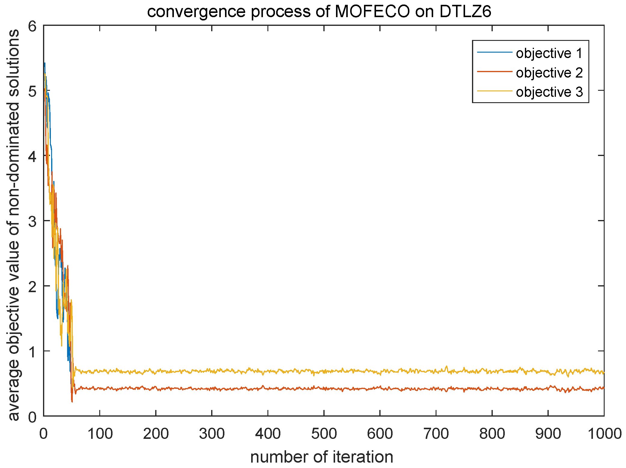
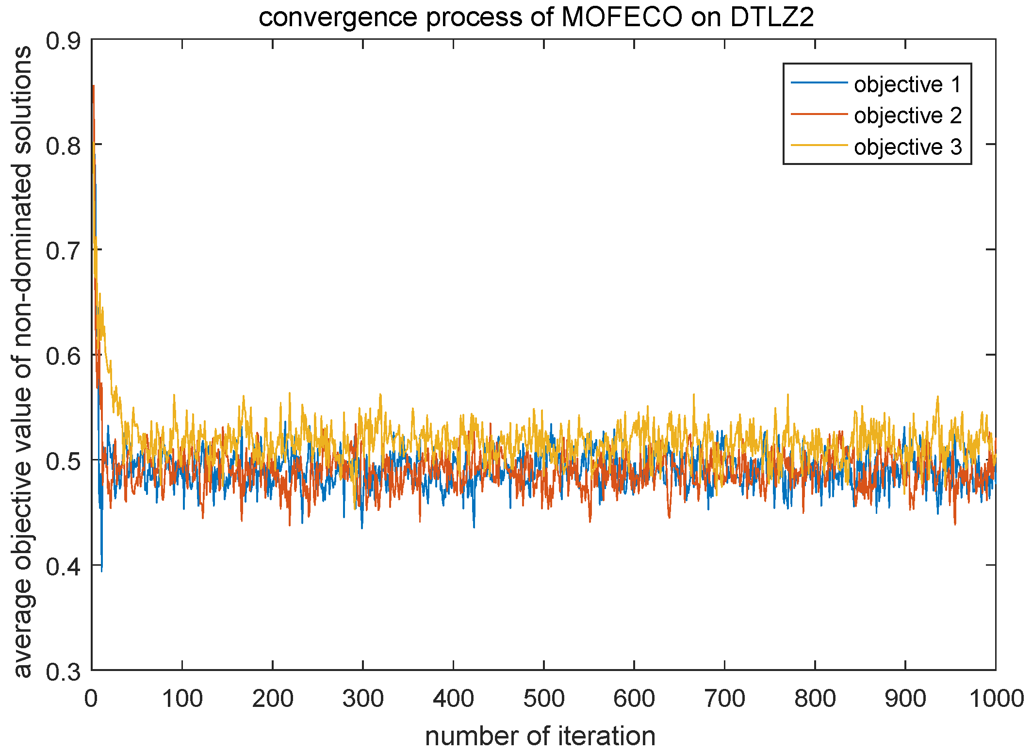
In order to more visually show the performance of the MOFECO algorithm, a detailed convergence process increasing the number of iterations is discussed. Here we choose two test problems DTLZ2 and DTLZ6 to show the convergence process. Experimental results are shown in Figure 30 and Figure 31. The abscissa represents the number of iterations and the ordinate represents the average objective function value of the non-dominated solutions in each iteration.

As can be seen from Figure 30 and Figure 31, the population obtained by MOFECO converges rapidly in every objective of DTLZ2 and DTLZ6, which reflect the good convergence of the proposed MOFECO algorithm.

Overall, the proposed MOFECO performs better than NSGA-II, MOPSO, PESA-II and KnEA on most of the test functions used in the above experiments in terms of metrics $GD$, $PD$, $HV$, $SP$ and $SI$, which indicates that MOFECO algorithm has better convergence and diversity in solving MOO problems. But MOFECO performs slightly worse on $SI$ indicator compared with NSLS, which will be one of the problems we need to investigate in the follow-up research.

6. Conclusions

A new multi-objective evolutionary algorithm called the Multi-Objective Five-Elements Cycle Optimization algorithm (MOFECO) for solving MOO problems is proposed in this paper and the validity of the MOFECO has been verified by using the test function sets ZDT, DTLZ, WFG and MaF. The main idea of MOFECO is that, at each iteration, we divide the initial population into q independent cycles and each cycle contains L elements, where $L\times q$ represents the population number and each element represents an individual in the population. In each cycle, the force applied to each element by the other four elements related to the mass of each element, while the mass is represented by the objective functions. Therefore, the value of the force indirectly reflects the pros and cons of an individual and judges whether the individual is updated. In our paper, in case of an update, the local update or the global update is selected according to the current local-global probability value $P_s$. Then, the combined mutation based on mutation probability $P_m$ is performed, that is, the uniform distribution mutation operator is used in the early iteration, and the Cauchy distribution mutation operator is used in the middle of the iteration, and the Gauss distribution mutation operator is used in the late iteration. Next, as the offspring individuals are stored in the child population, the child population is combined with the parent population and the next generation is selected from them by using a fast non-dominated sorting and crowded distance calculation method, and then generate the current non-dominated solution set. The operations above are repeated until the maximum number of iterations is reached and then the optimal Pareto solution set is output as the result of optimization.

In this paper, we compared the different values of L and q, different update conditions, the adaptive update probability $P_s$ and the different mutation methods as parameters and conditions that affect the performance of MOFECO algorithm. In addition, this paper compared the performance of MOFECO with five popular MOEAs NSGA-II, MOPSO, PESA-II, KnEA and NSLS on 15 test problems, and discussed the convergence process of MOFECO on DTLZ2 and DTLZ6. The results demonstrate that the proposed MOFECO significantly outperforms MOPSO and PESA-II in convergence, diversity and distribution, and performs better than all five comparative algorithms in convergence and diversity. The main weakness of MOFECO is that its distribution of the obtained Pareto solution set is slightly worse than the one obtained by NSLS. It is certain that there is no guarantee that the MOFECO algorithm will always show better characteristics on all test problems. The strengths and weaknesses of the algorithm should be further studied based on the characteristics of the test problems in future research.

References

1. Garcia, J.; Berlanga, A.; Molina Löpez, J.M. Effective Evolutionary Algorithms for Many-Specifications Attainment: Application to Air Traffic Control Tracking Filters. IEEE Trans. Evol. Comput. 2009, 13, 151–168. [Google Scholar] [CrossRef]
2. Zhang, X.; Tian, Y.; Jin, Y. A Knee Point-Driven Evolutionary Algorithm for Many-Objective Optimization. IEEE Trans. Evol. Comput. 2015, 19, 761–776. [Google Scholar] [CrossRef]
3. Deb, K.; Kalyanmoy, D. Multi-Objective Optimization Using Evolutionary Algorithms; John Wiley & Sons, Inc.: New York, NY, USA, 2001. [Google Scholar]
4. Srinivas, N.; Deb, K. Muiltiobjective Optimization Using Nondominated Sorting in Genetic Algorithms. Evol. Comput. 1994, 2, 221–248. [Google Scholar] [CrossRef]
5. Deb, K.; Agrawal, S.; Pratap, A.; Meyarivan, T. A Fast Elitist Non-dominated Sorting Genetic Algorithm for Multi-objective Optimization: NSGA-II. In Parallel Problem Solving from Nature PPSN VI; Springer: Berlin/Heidelberg, Germany, 2000; pp. 849–858. [Google Scholar] [CrossRef]
6. Junhua, Y.; Cuimei, B.O.; Jun, L.I.; Yan, H. Multi-objective Optimization of Methyl Acetate Hydrolysis Process Based on NSGA-II Algorithm. In Proceedings of the 30th Chinese Control Conference, Shenyang, China, 8–11 June 2018. [Google Scholar]
7. Zitzler, E.; Thiele, L. Multiobjective Evolutionary Algorithms: A Comparative Case Study and the Strength Pareto Approach. IEEE Trans. Evol. Comput. 2000, 3, 257–271. [Google Scholar] [CrossRef]
8. Zitzler, E.; Laumanns, M.; Thiele, L. SPEA2: Improving the Strength Pareto Evolutionary Algorithm. In Technical Report Tik-Report 103; Computer Engineering and Communication Networks Lab (TIK), Swiss Federal Institute of Technology (ETH): Zurich, Switzerland, 2001; pp. 95–100. [Google Scholar]
9. Wu, X.; Cao, W.; Wang, D.; Ding, M. Multi objective optimization based on SPEA for the microgrid energy dispatch. In Proceedings of the 30th Chinese Control Conference, Shenyang, China, 8–11 June 2018. [Google Scholar]
10. Corne, D.; Knowles, J.D.; Oates, M.J. The Pareto Envelope-Based Selection Algorithm for Multi-objective Optimisation. In Proceedings of the 6th International Conference on Parallel Problem Solving from Nature PPSN VI, Paris, Prance, 18–20 September 2000; Springer: Berlin/Heidelberg, Germany, 2000; pp. 839–848. [Google Scholar]
11. Corne, D.W.; Jerram, N.R.; Knowles, J.D.; Oates, M.J. PESA-II: Region-based Selection in Evolutionary Multiobjective Optimization. In Proceedings of the 3rd Annual Conference on Genetic and Evolutionary Computation, San Francisco, CA, USA, 7–11 July 2001; pp. 283–290. [Google Scholar]
12. Coello Coello, C.A.; Lechuga, M.S. MOPSO: A proposal for multiple objective particle swarm optimization. In Proceedings of the 2002 Congress on Evolutionary Computation, Honolulu, HI, USA, 12–17 May 2002; CEC’02 (Cat. No.02TH8600). Volume 2, pp. 1051–1056. [Google Scholar] [CrossRef]
13. Patil, M.B.; Naidu, M.N.; Vasan, A.; Varma, M.R.R. Water Distribution System Design Using Multi-Objective Particle Swarm Optimisation. arXiv 2019, arXiv:1903.06127. [Google Scholar]
14. Hashim, H.A.; Abido, M.A. Location Management in LTE Networks using Multi-Objective Particle Swarm Optimization. Comput. Netw. 2019, 157, 78–88. [Google Scholar] [CrossRef]
15. Chen, B.; Zeng, W.; Lin, Y.; Zhang, D. A New Local Search-Based Multiobjective Optimization Algorithm. IEEE Trans. Evol. Comput. 2015, 19, 50–73. [Google Scholar] [CrossRef]
16. Fan, L.; Zeng, J.; Xiahou, J.; Lin, S.; Zeng, W.; Lv, H. Multi-Objective Evolutionary Algorithm Based On Non-Dominated Sorting and Bidirectional Local Search for Big Data. IEEE Trans. Ind. Inform. 2017, 13, 1979–1988. [Google Scholar]
17. Li, M.; Yang, S.; Liu, X. Pareto or Non-Pareto: Bi-Criterion Evolution in Multi-Objective Optimization. IEEE Trans. Evol. Comput. 2016, 20, 645–665. [Google Scholar] [CrossRef]
18. Tian, Y.; Zhang, X.; Cheng, R.; Jin, Y. A multi-objective evolutionary algorithm based on an enhanced inverted generational distance metric. In Proceedings of the 2016 IEEE Congress on Evolutionary Computation (CEC), Vancouver, BC, Canada, 24–29 June 2016; pp. 5222–5229. [Google Scholar] [CrossRef]
19. Liu, M. Five-elements cycle optimization algorithm for the travelling salesman problem. In Proceedings of the 2017 18th International Conference on Advanced Robotics (ICAR), Hong Kong, China, 10–12 July 2017; pp. 595–601. [Google Scholar] [CrossRef]
20. Liu, M. Five-elements cycle optimization algorithm for solving continuous optimization problems. In Proceedings of the 2017 IEEE 4th International Conference on Soft Computing Machine Intelligence (ISCMI), Balaclava, Mauritius, 22–24 November 2017; pp. 75–79. [Google Scholar] [CrossRef]
21. Asafuddoula, M.; Ray, T.; Sarker, R. A Decomposition Based Evolutionary Algorithm for Many Objective Optimization. IEEE Trans. Evol. Comput. 2015, 19, 445–460. [Google Scholar] [CrossRef]
22. Schaffer, J.D. Some Experiments in Machine Learning Using Vector Evaluated Genetic Algorithms (Artificial Intelligence, Optimization, Adaptation, Pattern Recognition). Ph.D. Thesis, Vanderbilt University, Nashville, TN, USA, 1984. [Google Scholar]
23. Wen, S.; Zheng, J. Improved diversity maintenance strategy in NSGA-II. Comput. Eng. Appl. 2010, 46, 49–53. [Google Scholar]
24. Lei, R.; Cheng, Y. A pareto-based differential evolution algorithm for multi-objective optimization problems. In Proceedings of the 2010 Chinese Control and Decision Conference, Xuzhou, China, 26–28 May 2010; pp. 1608–1613. [Google Scholar] [CrossRef]
25. Wen, S. The Research on Mutation Operators for Multi-Objective Evolutionary Algorithms. Ph.D. Thesis, Xiangtan University, Xiangtan, China, 2009. [Google Scholar]
26. Schaffer, J.D. Multiple Objective Optimization with Vector Evaluated Genetic Algorithms. In Proceedings of the 1st International Conference on Genetic Algorithms, Pittsburgh, PA, USA, 24–26 July 1985; pp. 93–100. [Google Scholar]
27. Knowles, J.; Corne, D. The Pareto Archived Evolution Strategy: A New Baseline Algorithm for Pareto Multiobjective Optimisation. In Proceedings of the Congress on Evolutionary Computation, Washington, DC, USA, 6–9 July 1999. [Google Scholar] [CrossRef]
28. Kim, Y.; Street, W.N.; Menczer, F. An evolutionary multi-objective local selection algorithm for customer targeting. In Proceedings of the 2001 Congress on Evolutionary Computation (IEEE Cat. No.01TH8546), Seoul, Korea, 27–30 May 2001; pp. 759–766. [Google Scholar] [CrossRef]
29. Horn, J.; Nafpliotis, N.; Goldberg, D.E. A niched Pareto genetic algorithm for multiobjective optimization. In Proceedings of the First IEEE Conference on Evolutionary Computation, Orlando, FL, USA, 29 June–1 July 1994; pp. 82–87. [Google Scholar] [CrossRef]
30. Fonseca, C.M.; Fleming, P.J. Genetic Algorithms for Multiobjective Optimization: FormulationDiscussion and Generalization. In Proceedings of the 5th International Conference on Genetic Algorithms, Urbana-Champaign, IL, USA, 17–21 July 1993; pp. 416–423. [Google Scholar]
31. Wagner, M.; Neumann, F. A Fast Approximation-guided Evolutionary Multi-objective Algorithm. In Proceedings of the 15th Annual Conference on Genetic and Evolutionary Computation, Amsterdam, The Netherlands, 6–10 July 2013; pp. 687–694. [Google Scholar] [CrossRef]
32. Zitzler, E.; Künzli, S. Indicator-Based Selection in Multiobjective Search. In Parallel Problem Solving from Nature—PPSN VIII; Springer: Berlin/Heidelberg, Germany, 2004; pp. 832–842. [Google Scholar] [CrossRef]
33. Deb, K.; Jain, H. An Evolutionary Many-Objective Optimization Algorithm Using Reference-Point-Based Nondominated Sorting Approach, Part I: Solving Problems With Box Constraints. IEEE Trans. Evol. Comput. 2014, 18, 577–601. [Google Scholar] [CrossRef]
34. Li, K.; Deb, K.; Zhang, Q.; Kwong, S. An Evolutionary Many-Objective Optimization Algorithm Based on Dominance and Decomposition. IEEE Trans. Evol. Comput. 2015, 19, 694–716. [Google Scholar] [CrossRef]
35. Kennedy, J.; Eberhart, R. Particle swarm optimization. In Proceedings of the ICNN’95—International Conference on Neural Networks, Perth, Australia, 27 November–1 December 1995; pp. 1942–1948. [Google Scholar] [CrossRef]
36. Lin, D.; Li, M.Q.; Kou, J.S. Research of mutation operator in evolutionary programming and evolutionary strategies. J. Tianjin Univ. Sci. Technol. Ed. 2000, 33, 627–630. [Google Scholar]
37. Zitzler, E.; Deb, K.; Thiele, L. Comparison of Multiobjective Evolutionary Algorithms: Empirical Results. Evol. Comput. 2000, 8, 173–195. [Google Scholar] [CrossRef]
38. Deb, K.; Thiele, L.; Laumanns, M.; Zitzler, E. Scalable Test Problems for Evolutionary Multiobjective Optimization. In Evolutionary Multiobjective Optimization: Theoretical Advances and Applications; Springer: London, UK, 2005; pp. 105–145. [Google Scholar] [CrossRef]
39. Huband, S.; Hingston, P.; Barone, L.; While, L. A review of multiobjective test problems and a scalable test problem toolkit. IEEE Trans. Evol. Comput. 2006, 10, 477–506. [Google Scholar] [CrossRef]
40. Cheng, R.; Li, M.; Tian, Y.; Zhang, X.; Yang, S.; Jin, Y.; Yao, X. A benchmark test suite for evolutionary many-objective optimization. Complex Intell. Syst. 2017, 3, 67–81. [Google Scholar] [CrossRef]
41. Ye, T.; Ran, C.; Zhang, X.; Jin, Y. PlatEMO: A MATLAB Platform for Evolutionary Multi-Objective Optimization. IEEE Comput. Intell. Mag. 2017, 12, 73–87. [Google Scholar] [CrossRef]
42. Wang, Y.N.; Wu, L.H.; Yuan, X.F. Multi-objective self-adaptive differential evolution with elitist archive and crowding entropy-based diversity measure. Soft Comput. 2010, 14, 193–209. [Google Scholar] [CrossRef]
43. Vanveldhuizen, D.A.; Lamont, G.B. Evolutionary computation and convergence to a Pareto front. In Proceedings of the Late Breaking Papers at the Genetic Programming 1998 Conference, Stanford University, CA, USA, 13–16 July 1998; pp. 221–228. [Google Scholar]
44. Schott, J.R. Fault Tolerant Design Using Single and Multi-Criteria Genetic Algorithm Optimization. Ph.D. Thesis, Massachusetts Institute of Technology, Cambridge, MA, USA, 1995. [Google Scholar]
45. Solow, A.; Polasky, S.; Broadus, J. On the Measurement of Biological Diversity. J. Environ. Econ. Manag. 1993, 24, 60–68. [Google Scholar] [CrossRef]
46. While, L.; Hingston, P.; Barone, L.; Huband, S. A faster algorithm for calculating hypervolume. IEEE Trans. Evol. Comput. 2006, 10, 29–38. [Google Scholar] [CrossRef]
47. Zitzler, E.; Thiele, L.; Laumanns, M.; Fonseca, C.M.; Fonseca, V.G.D. Performance Assessment of Multiobjective Optimizers: An Analysis and Review. IEEE Trans. Evol. Comput. 2003, 7, 117–132. [Google Scholar] [CrossRef] [Green Version]
Figure 1. Pareto optimal solutions (a,b,c,d,e,f) and dominated solutions (g,h,i,j,k,l).
Algorithms 12 00244 g001
Figure 2. The generating and restricting interactions between the five elements.
Algorithms 12 00244 g002
Figure 3. The flowchart of MOFECO algorithm.
Algorithms 12 00244 g003
Figure 4. Nonlinear variation of P s .
Algorithms 12 00244 g004
Figure 5. Linear variation of P s .
Algorithms 12 00244 g005
Figure 6. Pareto front of MOFECO on ZDT1.
Algorithms 12 00244 g006
Figure 7. Pareto front of MOFECO on ZDT2.
Algorithms 12 00244 g007
Figure 8. Pareto front of MOFECO on ZDT4.
Algorithms 12 00244 g008
Figure 9. Pareto front of MOFECO on ZDT6.
Algorithms 12 00244 g009
Figure 10. True Pareto front on DTLZ2.
Algorithms 12 00244 g010
Figure 11. Pareto front of MOFECO on DTLZ2.
Algorithms 12 00244 g011
Figure 12. True Pareto front on DTLZ4.
Algorithms 12 00244 g012
Figure 13. Pareto front of MOFECO on DTLZ4.
Algorithms 12 00244 g013
Figure 14. True Pareto front and Pareto front of MOFECO on DTLZ5.
Algorithms 12 00244 g014
Figure 15. True Pareto front and Pareto front of MOFECO on DTLZ6.
Algorithms 12 00244 g015
Figure 16. True Pareto front on DTLZ7.
Algorithms 12 00244 g016
Figure 17. Pareto front of MOFECO on DTLZ7.
Algorithms 12 00244 g017
Figure 18. True Pareto front on WFG2.
Algorithms 12 00244 g018
Figure 19. Pareto front of MOFECO on WFG2.
Algorithms 12 00244 g019
Figure 20. True Pareto front on WFG3.
Algorithms 12 00244 g020
Figure 21. Pareto front of MOFECO on WFG3.
Algorithms 12 00244 g021
Figure 22. True Pareto front on WFG4.
Algorithms 12 00244 g022
Figure 23. Pareto front of MOFECO on WFG4.
Algorithms 12 00244 g023
Figure 24. True Pareto front on MaF1.
Algorithms 12 00244 g024
Figure 25. Pareto front of MOFECO on MaF1.
Algorithms 12 00244 g025
Figure 26. True Pareto front on MaF2.
Algorithms 12 00244 g026
Figure 27. Pareto front of MOFECO on MaF2.
Algorithms 12 00244 g027
Figure 28. True Pareto front on MaF12.
Algorithms 12 00244 g028
Figure 29. Pareto front of MOFECO on MaF12.
Algorithms 12 00244 g029
Figure 30. Convergence process of MOFECO on DTLZ2.
Algorithms 12 00244 g030
Figure 31. Convergence process of MOFECO on DTLZ6.
Algorithms 12 00244 g031