Article

Comparison and Interpretation Methods for Predictive Control of Mechanics

Department of Mechanical Engineering (CVN), Columbia University, New York, NY 10027, USA
Algorithms 2019, 12(11), 232; https://doi.org/10.3390/a12110232
Submission received: 20 August 2019 / Revised: 28 October 2019 / Accepted: 1 November 2019 / Published: 4 November 2019
(This article belongs to the Special Issue Model Predictive Control: Algorithms and Applications)

Abstract

:
Objects that possess mass (e.g., automobiles, manufactured items, etc.) translationally accelerate in direct proportion to the force applied scaled by the object’s mass in accordance with Newton’s Law, while the rotational companion is Euler’s moment equations relating angular acceleration of objects that possess mass moments of inertia. Michel Chasles’s theorem allows us to simply invoke Newton and Euler’s equations to fully describe the six degrees of freedom of mechanical motion. Many options are available to control the motion of objects by controlling the applied force and moment. A long, distinguished list of references has matured the field of controlling a mechanical motion, which culminates in the burgeoning field of deterministic artificial intelligence as a natural progression of the laudable goal of adaptive and/or model predictive controllers that can be proven to be optimal subsequent to their development. Deterministic A.I. uses Chasle’s claim to assert Newton’s and Euler’s relations as deterministic self-awareness statements that are optimal with respect to state errors. Predictive controllers (both continuous and sampled-data) derived from the outset to be optimal by first solving an optimization problem with the governing dynamic equations of motion lead to several controllers (including a controller that twice invokes optimization to formulate robust, predictive control). These controllers are compared to each other with noise and modeling errors, and the many figures of merit are used: tracking error and rate error deviations and means, in addition to total mean cost. Robustness is evaluated using Monte Carlo analysis where plant parameters are randomly assumed to be incorrectly modeled. Six instances of controllers are compared against these methods and interpretations, which allow engineers to select a tailored control for their given circumstances. Novel versions of the ubiquitous classical proportional-derivative, “PD” controller, is developed from the optimization statement at the outset by using a novel re-parameterization of the optimal results from time-to-state parameterization. Furthermore, time-optimal controllers, continuous predictive controllers, and sampled-data predictive controllers, as well as combined feedforward plus feedback controllers, and the two degree of freedom controllers (i.e., 2DOF). The context of the term “feedforward” used in this study is the context of deterministic artificial intelligence, where analytic self-awareness statements are strictly determined by the governing physics (of mechanics in this case, e.g., Chasle, Newton, and Euler). When feedforward is combined with feedback per the previously mentioned method (provenance foremost in optimization), the combination is referred to as “2DOF” or two degrees of freedom to indicate the twice invocation of optimization at the genesis of the feedforward and the feedback, respectively. The feedforward plus feedback case is augmented by an online (real time) comparison to the optimal case. This manuscript compares these many optional control strategies against each other. Nominal plants are used, but the addition of plant noise reveals the robustness of each controller, even without optimally rejecting assumed-Gaussian noise (e.g., via the Kalman filter). In other words, noise terms are intentionally left unaddressed in the problem formulation to evaluate the robustness of the proposed method when the real-world noise is added. Lastly, mismodeled plants controlled by each strategy reveal relative performance. Well-anticipated results include the lowest cost, which is achieved by the optimal controller (with very poor robustness), while low mean errors and deviations are achieved by the classical controllers (at the highest cost). Both continuous predictive control and sampled-data predictive control perform well at both cost as well as errors and deviations, while the 2DOF controller performance was the best overall.

1. Introduction

Michel Chasles’s Theorem [1] allows us to simply invoke Euler’s [2] and Newton’s [3] equations to fully describe the six degrees of freedom of mechanical motion. Controlling mechanical motion has an even longer pedigree. The issue of automatic control of mechanical motion has occupied engineers for hundreds of years. Consider the Greeks and Arabs as early as 300 BC to about 1200 AD. They used float regulators for water clocks [4]. Imagine the float in a toilet reservoir. When the reservoir tank levels reached the desired levels, floats would actuate releases to keep the water at that level. This guaranteed a constant flow rate from one tank to a second tank. The time it takes to fill the second tank at this constant flow rate was a constant clock. Perhaps feedback was born in this way if not earlier. The period prior to 1900 is often referred to as the primitive period of automatic controls. The period from 1900 to the 1960s can be considered the classical period, while the 1960s through present time is often referred to as the modern period of automatic controls [5]. By the 1840s, automatic controls were examined mathematically through differential equations (e.g., British astronomer G.B. Airy’s feedback pointed telescope [6] was developed using mathematical stability analysis). By the 1920s and 1930s, the difficulty in dealing with differential equations led to the development of frequency domain techniques driving the analysis of automatic control systems via such tools as gain and phase margins measured on frequency response plots [6]. While some work was done with stochastic analysis (e.g., Wiener’s 1949 statistically optimal filter [7]), it was in the 1960s that time-domain differential equations re-emerged in strength. By 1957, Bellman had solved optimum control problems backwards in time [8]. Meanwhile Pontryagin used Euler’s calculus of variations to develop his maximum principle to solve optimization problems [9,10]. Around this same time, Kalman developed equations for an estimator [11] that proved equivalent to the linear quadratic regulator (LQR) [12]. Kalman demonstrated that time-domain approaches are more applicable for linear and non-linear systems (especially when dealing with multi-input/output systems). Kalman formalized the optimality of control by minimizing a general quadratic cost function. Subsequent to the establishment of optimal benchmarks, adaptive [13,14,15,16,17,18,19,20] and learning controls [21,22,23,24,25,26,27,28,29,30,31,32] arose with a subsequent effort to combine the two, which makes adaptive controllers optimal, where optimization occurs after first establishing the control equation, such as by using ‘approximate’ dynamic programming [33]. Assuming distributed models, Reference [34] and Reference [35] used neighbor-based optimization to develop predictive controls. Other researchers [36] sought extensions into nonlinear systems with actuator failures, while Reference [37] tried to use neural networks to find the model and response in a predictive topology. Inspired by the adaptive lineages [13,14,15,16,17,18,19,20,21,22,38] and learning lineages [23,24,25,26,27,28,29,30,31,32], both Reference [39] and Reference [40] break with the usual design paradigm and, instead, begin with the solution of a nonlinear optimization problem as the first step of control design, and that an alternative paradigm is adopted in this study, which results in controllers’ instances leading to a novel proposal: a two degree of freedom controller that results from the original optimization statement including predictive control and robust feedback control achieving non-trivial results in the face of noise modeling errors not expressly written in the original problem formulation. The achievement of good results despite a dramatic simplification of methods is original and refreshing.
Over 25 years ago, in 1993, Lee et al. formulated a nonlinear model predictive control algorithm based on successive linearization, where the extended Kalman filter uses a multi-step future state prediction [41] Almost 10 year later, in 2002, Wang et al. [42] proposed an optimal model predictive control for high order plants modeled first-order linear systems with time-delay and random disturbance including non-gaussian noise, while the Kalman filter was used for present and future state estimation. By 2007, model predictive control (MPC) with Kalman filters was appearing in undergraduate theses [43]. Published in 2012, Reference [44] deals with the closed-loop robust stability of nonlinear model predictive control (NMPC) coupled with an extended Kalman filter (EKF) where optimization was used for target setting used in the objective function in nonlinear model predictive control, while, unfortunately, stability deteriorates due to the estimation error. In 2013, predictive control was used for the constrained Hammerstein-Wiener model of nonlinear chemical processes (e.g., continuous stirred tank reactors) with a Kalman filter for output feedback of a linear subsystem elaborated from a finite horizon through the receding horizon [45]. In that same year, Reference [46] focused on state estimation, comparing the Kalman filter and the Particle Filter, while state estimation with finite state models was also briefly considered. The Bayesian approach was emphasized.
In 2016, Binette et al. sought to improve economic performance of batch processes using the Nonlinear Model Predictive Control (NMPC) without parameter adaptation, where the measured states serve as new initial conditions for the re-optimization problem with a diminishing horizon. Model mismatch of the plant preclude achievement of optimality. However, neglecting process noise and assuming small parametric variations, re-optimization always improves performance assuming the trajectory is feasible and, thus, Binette et al. assert that this illustrates robustness. This manuscript will re-examine this goal instead of seeking to achieve robustness by including feedback that directly derives from the original optimization problem (whose results are codified in time-parameters rather than state parameters). [47] Cao et al. represented uncertainties using scenarios from a robust nonlinear model’s predictive control strategy, where large-scale stochastic programming is used at each sampling instance solved by the parallel Schur complement method. The method merely exceeds the robustness of an open-loop optimal control, and, furthermore, processing time remains a limitation while achieving an optimal update only twice per minute. [48] Genesh et al. used a model predictive control system developed to control furnace exit temperature to prevent parts from overheating in a quench hardening process. Knowing only a proportional state and time, a mere 5.3% efficiency increase was achievable [49].
In 2017, Jost et al. used nonlinear model predictive control combined with parameter and state estimation techniques to provide dynamic process feedback to counter uncertainty. To counter uncertainty, ubiquitous dual methods provide excitation with the control while minimizing a given objective. Jost et al. proposed to sequentially solve robust optimal control, optimal experimental design, and state and parameter estimation problems separating the control and experimental design problems, and permitting independent analysis of sampling. This proved very useful when fast feedback was needed. One such case is the Lotka-Volterra fishing benchmark where the Jost algorithm indicates a 36% reduction of parameter [50]. Xu et al. used the Discrete Mechanics and Optimal Control (DMOC) method to formulate a nonlinear model predictive control, using numerical simulations to compare with the standard nonlinear model predictive control (NMPC) formulation based on the method of multiple-shooting. Using the Real-Time Iteration scheme, the real-time application of the NMPC algorithm extended the DMOC based NMPC applied to the swing-up and stabilization task of a double pendulum on a cart with limited rail length to show its capability for controlling nonlinear dynamical systems with input and state constraints [51]. Suwartadi et al. presented a sensitivity-based predictor-corrector path-following algorithm for fast nonlinear model predictive control (NMPC) and demonstrated it on a large case study with an economic cost function solving a sequence of quadratic programs to trace the optimal nonlinear model’s predictive control solution along a parameter change incorporating strongly-active inequality constraints included as equality constraints in the quadratic programs, while the weakly-active constraints are left as inequalities [52]. Vaccari et al. designed an economic model’s predictive control to asymptotically achieve optimality in the presence of plant-model mismatch using an offset-free disturbance model and to modify the target optimization problem with a correction term that is iteratively computed to enforce the necessary conditions of optimality in the presence of a plant-model mismatch [53].
Last year, in 2018, Kheradmandi et al. addressed a data-driven model-based economic model and predictive control capable of stabilizing a system at an unstable equilibrium point [54]. Wong et al. applied model predictive control to pharmaceutical manufacturing operations using physics-based models akin to the technique adopted in this study from deterministic artificial intelligence [37]. Durand et al. developed a nonlinear systems framework for understanding cyberattack-resilience of process and control designs and indicates through an analysis of three control designs for resiliency [55]. Singh Sidhu utilized model predictive control for hydraulic fracturing based on the physics-based assumptions that the rock mechanical properties, such as the Young’s modulus, are known and spatially homogenous, where optimality is forsaken if there is an uncertainty in the rock mechanical properties by proposing an approximate dynamic programming-based approach. This is a model-based control technique, which combines a high-fidelity simulation and function approximate to alleviate the “curse-of-dimensionality” associated with the traditional dynamic programming approach [33]. Xue et al. addressed the problem of fault-tolerant stabilization of nonlinear processes subject to input constraints, control actuator faults, and limited sensor–controller communication by using the fault-tolerant Lyapunov-based model [36]. Tian et al. applied model predictive control design for a mineral column flotation process modeled by a set of nonlinear coupled hetero-directional hyperbolic partial differential equations (PDEs) and ordinary differential equations (ODEs), which accounts for the interconnection of well-stirred regions represented by continuous stirred tank reactors (CSTRs) and transport systems given by hetero-directional hyperbolic PDEs, with these two regions combined through the PDEs boundaries. Cayley–Tustin time discretization transformation was used to develop a discrete model’s predictive control. In this article, discretization delays are implemented alone without specified treatment to evaluate their deleterious effects on the control’s accuracy and robustness [56]. Gao et al. considered a distributed model predictive controller on a class of large-scale systems, which is composed of many interacting subsystems. Each of them is controlled by an individual controller where, by integrating the steady-state calculation, the designed controller proved able to guarantee the recursive feasibility and asymptotic stability of the closed-loop system in the cases of both tracking the set point and stabilizing the system to zeroes [34]. Wu et al. utilized an economic model’s predictive control on a nonlinear system class with input constraints for chemical seeking to first guarantee stability, and then ensure optimality (this is the opposite approach taken in this manuscript) [57]. Liu et al. proposed an economic model’s predictive control with zone tracking based on economic performance and reachability of the optimal steady-state by decoupling dynamic zone tracking and economic objectives to simplify parameter tuning [58]. Zhang et al. sought to augment dissipative theory to propose a novel distributed control framework to simultaneously optimize conflicting cost statements in demand-side management schemes (e.g., building air conditioning), while seeking to mitigate power fluctuations. Their proposed method achieved the objective of renewable intermittency mitigation through proper coordination of distributed controllers, and the solution proved to be scalable and computationally efficient [35]. Bonfitto et al. presented a linear offset-free model predictive controller applied to active magnetic bearings, which exploits the performance and stability advantages of a classical model-based control while overcoming the effects of the plant-model mismatch on reference tracking by incorporating a disturbance observer to augment the plant model equations. Effectiveness of the method was demonstrated in terms of the reference tracking performance, cancellation of plant-model mismatch effects, and low-frequency disturbance estimation [59]. Godina et al. compared model predictive control to bang-bang control and proportional-integral-derivative control of home air conditioning seeking to minimize energy consumption assuming six time-of-use electricity cost rates during an entire summer, while tariff (taxation) rates were evaluated for efficacy [60].
Lastly, this year (in 2019), Khan et al. described a model predictive control based on the technique of a finite control set applied to uninterrupted power supply systems, where the system’s mathematical model is used to predict voltages of each switch at each sampling time applied to switching states of parallel inverters. They achieved a low computational burden, good steady state performance, fast transient response, and robust results against parameter disturbances as compared to linear control [61]. Since variable switching frequency negatively impacts output filters, Yoo et al. implemented constant switching frequency in a finite control-set model predictive controller based on the gradient descent method to find optimal voltage vectors. They found lower total harmonic distortion in output current with improved computation times [62]. Zhang et al. utilized sequential model predictive control for power electronic AC converter, and their research sought to improve a complicated weighting factor design and also computational burden applied to three-phase direct matrix conversion. The performance akin nominal model’s predictive control was revealed [63]. Baždarić et al. introduced approaches to the predictive control of a DC-DC boost converter in a comparison of the controllers that consider all of the current objectives and minimize the complexity of the online processing, which results in an alternative way of building the process model based on the fuzzy identification that contributes to the final objective. This includes the applicability of the predictive methods for fast processes [64]. Seeking to optimize the control strategy of the traction line-side converter (LSC) in high-speed railways, Wang et al. applied a model-based predictive current control and the results indicate a significant influence on the performance of traditional transient direct current control. Both the oscillation pattern and the oscillation peak under traditional transient direct current control can be easily influenced when these parameters change [65].
In 2019, Maxim et al. [66] investigated how, when, and why to choose model predictive control over proportional-integral-derivative control. With this backdrop, the goal of the research presented in this manuscript is to develop and then examine several variations of classical and modern era optimal controllers and compare their performance against each other.
A key contribution is the design of predictive controllers that are designed using optimization as the very first step, including a formulation of state feedback for robustness in the same optimization while a subsequent step converts the optimal solution from time-parameterization to state-parameterization allowing proportional-derivative gains to be expressed as exact functions of the optimal solution. Thus, feedback errors are de facto expressed exactly in terms of the solutions to the original optimization problem and errors are, thereby, optimally rejected. This notion permits the reader to use only this predictive, optimal feedback controller by itself and also together with the optimal feedforward. Lastly, comparing the optimal feedforward to the predictive optimal feedback control permits expression of a proposed controller called “2DOF” to imply the twice-invocation of the original optimization problem. This proposed 2DOF topology achieves near-machine precision target tracking errors while using near-minimal costs.
Despite the previously mentioned lengthy lineage of smoothing estimators to eliminate negative effects of noise (e.g., control chattering), a distinguishing feature presented in this case is the production of state estimates as an output of the original optimization problem, which alleviates the need for state estimation, which is often performed in the literature by various realizations of Kalman filters. In this case, the noisy states provided by sensors will not be smoothed by optimal estimators (e.g., Kalman filters), instead left in full-effect as agitators of deleterious effects in order to critically compare the robustness of each approach compared. The same is true of modeling errors: the effects were purposefully left out of the original problem formulation, yet applied in the validating simulations to critically expose the strengths and weaknesses of each approach compared.

2. Materials and Methods

This section derives and describes the implementation of the controllers in this study including Optimum Open Loop, Continuous Predictive Optimum, Sampled Predictive Optimum, proportional-derivative (PD), Feedforward/Feedback PD, and 2DOF control. The context of the already commonly defined term “feedforward” used here (differently and more restrictively) is the context of deterministic artificial intelligence, where analytical self-awareness statements are strictly determined by the governing physics (of mechanics in this case, e.g. Chasle, Newton, and Euler). When the feedforward is combined with proportional-derivative, “PD” feedback control (developed from the optimization statement at the outset using a novel re-parameterization of the time-optimal results from time-to-state parameterization), the resulting controller is referred to here as “2DOF” or two degrees-of-freedom to indicate the twice invocation of optimization at the genesis of the feedforward and the feedback, respectively.
First, a brief derivation of the optimum control for our double integrator assumes a quadratic cost function. Using a simple double-integrator plant (modeling translational motion in an inertial reference frame described by Newton and Chasle), controllers were developed in accordance with the new design techniques to travel from the initial conditions ( θ ( 0 ) = 0 , ω ( 0 ) = 0 ) to the final conditions ( θ ( 1 ) = 1 , ω ( 1 ) = 0 ) , where θ is the translational motion state and ω is the translational velocity state. The controllers were then applied to a mismodeled plant, which contained a 0.005 [ I ] { ω 2 } dependence (where I is the mass inertia and ω is angular velocity). Additionally, the inertia of a body is difficult to know exactly what adds “inertia noise,” which is also referred to as modeling errors. After witnessing the deleterious impact of noise on an open loop controller’s robustness, the remaining controllers studied in this research were closed loop. Feedback was instituted to deal with noise. Figures of merit address two key issues of control: achieving desired end conditions and minimizing the required control effort. Accordingly, controllers in this research report will be compared via nominal error norms (for θ, ω, and cost) and via statistical analysis of random variation (mean error, deviation, and mean cost).
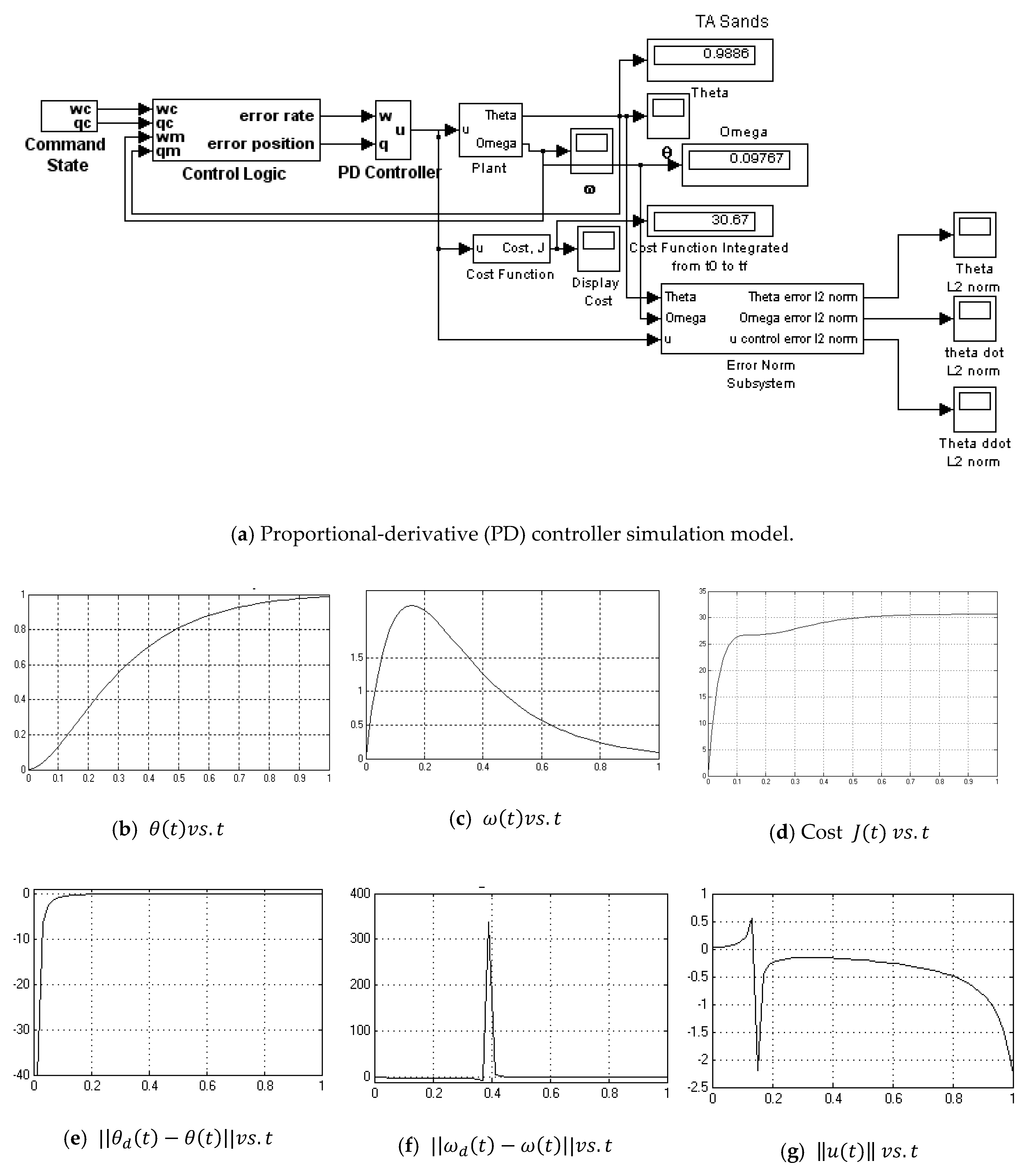
Quadratic cost was evaluated for each controller, where every controller’s model coded in MATLAB/SIMULINK is depicted in the Appendix A to aide repeatability for the reader. End conditions were compared via error norms (specifically ℓ2, also known as least squares). The controllers were designed to both meet the end conditions and minimize the cost function (often opposing goals) from the outset. Designs were iterated to get as close as possible to the end conditions while keeping cost low (a ubiquitous trade-off). In the main body of the manuscript, each controller is designed with descriptions to address the key issues of control in addition to how well they perform in a Monte Carlo analysis.
It will be shown that the optimum control for our double integrator is u = a t + b , and this is simply a generalized form that can be narrowed to u = K p ( 1 t ) θ + K v ( 1 t ) θ ˙ (looks somewhat like a classical PD controller). This research implements the optimum control in several manners: Open loop, Continuous-predictive, Sampled-Predictive, Feedforward/feedback, and 2 Degree-of-freedom (2DOF). Thus, the predictive controllers are derived from optimality rather than the opposite.

2.1. Open Loop Optimum Controller

This section derives the optimum control from first principles: standard articulation of an optimization problem. While, subsequent derivation of innovative control architectures uses the optimum control developed in this section, this explanation will not be repeated in subsequent discussions. The optimum controller uses optimization theory to address the key control issue of cost. The optimum controller is defined as the one that minimizes the quadratic control cost function. To find an optimum controller, we choose to optimize the double integrator cost J and the square of the control as a function of all variables annotated ( · ) as follows.
Minimize   J [ θ ( · ) , ω ( · ) , u ( · ) ] = 1 2 t 0 t f u 2 d t .
Subject   to   θ ˙ = ω
ω ˙ = u
θ ˙ = ω
( θ 0 , ω 0 ) = ( 0 , 0 )
( θ f 1 , ω f 1 , t f 1 ) = ( 0 , 0 , 0 )
Make some important observations. First, notice the notation. θ ( · ) , ω ( · ) , u ( · ) live in infinite dimensional functional space, while θ ( t ) , ω ( t ) , u ( t ) live in finite dimensional space. In addition, the smooth terminal manifold is the following: e ( θ f , t f ) = 0 . We intend to minimize the control Hamiltonian.
  • Write the control Hamiltonian.
    H ( λ , θ , u , t ) = F ( θ , u , t ) + λ T f ( θ , u , t )
  • Implement the Hamiltonian Minimization Condition for the static problem of Equation (8).
    min H ( ; u )   w h e r e   u R ,   t h a t   i s   H u = 0
    This is a constrained minimization problem, so use Equations (9) and (10) where λ ω is the Lagrange multiplier associated with the co-state.
    H ( ; u ) u = u + λ ω = 0
    u ( λ ω ) = λ ω
    Confirm optimality by verifying the convexity condition in Equation (11).
    2 H ( ; u ) u 2 = 1 > 0
    The result: once we find the co-state, we will have optimum control. Notice Karush-Kuhn-Tucker conditions often used with inequality constraints are not necessary here.
  • Apply the Adjoint Equations per Equations (12) and (14), which result in Equations (13) and (15), respectively, and are plotted in Figure 1b.
    λ ˙ θ = H θ = 0
    λ θ = a
    λ ˙ ω = H ω = λ θ = a
    Integrating (14)
    λ ω = at + b
  • Rewrite the Hamiltonian Minimization Condition in Equation (8) by substituting Equation (9).
    H u = u + λ ω = 0 u = λ ω
  • Substituting Equation (15) into Equation (16) produces Equation (17).
    Optimal   control ,   u u = at + b
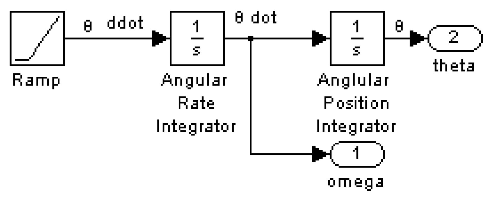
  • Implement in SIMULINK as displayed in Figure 2 using Equations (3), (18)–(20), which are simulated per Figure 2 and whose results are plotted in Figure 1a.
    u = θ ¨ = ω ˙ = a t + b
    ω = θ ˙ = θ ¨ d t = ( a t + b ) d t = a 2 t 2 + b t + c
    θ = θ ˙ d t = ( a t 2 + b t + c ) d t = a 6 t 3 + b 2 t 2 + c t + d
Equation (17) will be the enforced form of the control in subsequent derivations substantiating the novel paradigm contribution for each subsequent form. Using the initial conditions θ ( 0 ) = 0 , ω ( 0 ) = 0 and the final conditions θ ( 1 ) = 1 ,   ω ( 1 ) = 0 yields the values for constants: a = −12, b = 6, c = 0, and d = 0. Thus, the optimum open loop controller is Equation (21) implemented in SIMULINK, as depicted in Figure 2.
u o p e n l o o p = 12 t + 6
It is important to remember that u = 12 t + 6 is not the global optimum for the simple double integrator. We established the values a = −12, and b = 6 using the boundary values stated, which makes this a local optimum control from 0 t 1 . The more general u = a t + b is the global optimum control.
ASIDE: We’ll see in the next section how to implement the more general optimum control and solve for constants a and b as time, t progresses. That controller is referred to as the continuous predictive optimal closed-loop controller.
Notice in Figure 1 the behavior of the extremal states, co-states (in shadow space), and control in the figures below are limited to 0 t 1 . Observe that the state θ is nonlinear in normal space, while the co-state is linear and sloped. Similarly, the state ω is nonlinear in normal space, while the co-state is linear and sloped. Additionally, notice the figure displayed in Figure 2 is provided in full form in the Appendix A. In addition to the simple double integrator implementation of the optimum control, there are subsystems to calculate the resultant cost as well as J and subsystems to display the data numerically and via plots. This format has been maintained throughout analysis of all the controllers considered in this study.

2.2. Continuous Predictive Closed Loop Optimum Controller

This section briefly describes the implementation of a feedback optimum controller where the constants of integration are continuously calculated by the controller instantaneously. The basis of the derivation begins with the previously mentioned solution to the optimization problem, substantiating a novel contribution. Recall from the previous section, Equation (21) u = 12 t + 6 is not the global optimum controller. As time progresses, the boundary conditions used to solve Equation (17) u = a t + b change. Additionally, the starting position changes due to movement, noise, and uncertainties. This and subsequent controllers implement the optimum control using feedback to deal with changing boundary conditions. Rather than command the controller using the local optimum solution in Equation (21), instead use the global optimal solution in Equation (17) with full state feedback. Using the present state as the new initial boundary value, we solve for the constants of integration of the general optimum control in Equation (17). Recall that a = −12 and b = 6 resulted from the specified initial and final conditions. As time progresses, this continuous predictive (closed loop) optimum controller will calculate new a’s and b’s using its present time as the initial condition.
  • Recall Equations (18)–(20) where θ ( 1 ) = 1 , ω ( 1 ) = 0 yields:
    θ { 1 } = a 6 ( 1 ) + b 2 ( 1 ) + c ( 1 ) + d = a 6 + b 2 + c + d = 1
    ω ( 1 ) = a 2 ( 1 ) + b ( 1 ) + c = a 2 + b + c = 0
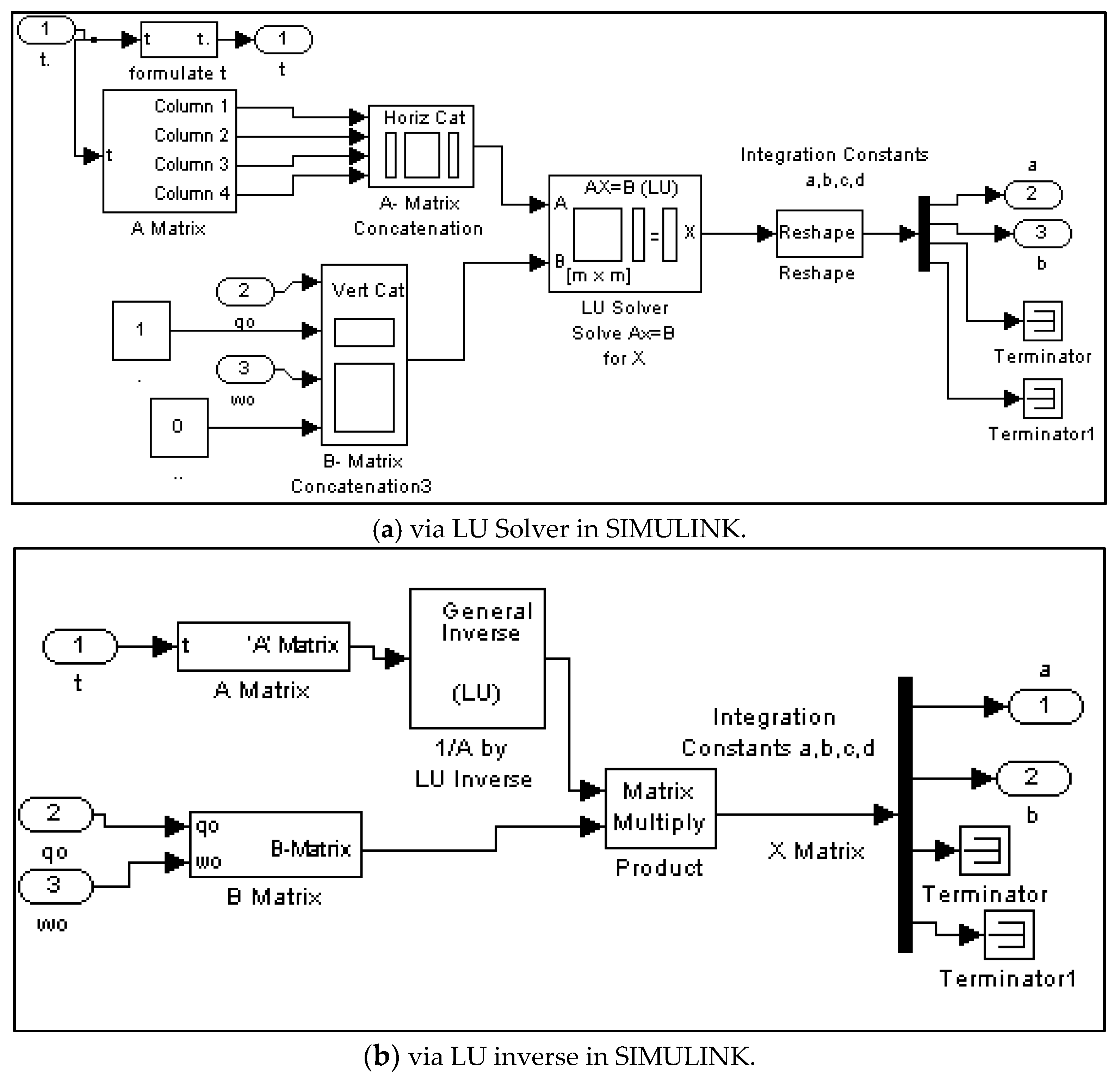
  • Set up a matrix equation in the form [ A ] { x } = { B } simulated in Figure 3.
    [ t 0 3 6 t 0 2 2 t 0 1 1 6 1 2 1 1 t 0 2 2 t 0 1 1 1 2 1 1 0 ] [ A ] { a b c d } { x } = { θ ( 0 ) 1 ω ( 0 ) 0 } { B } { x } = [ A ] { B } { x ( 1 ) x ( 2 ) x ( 3 ) x ( 4 )
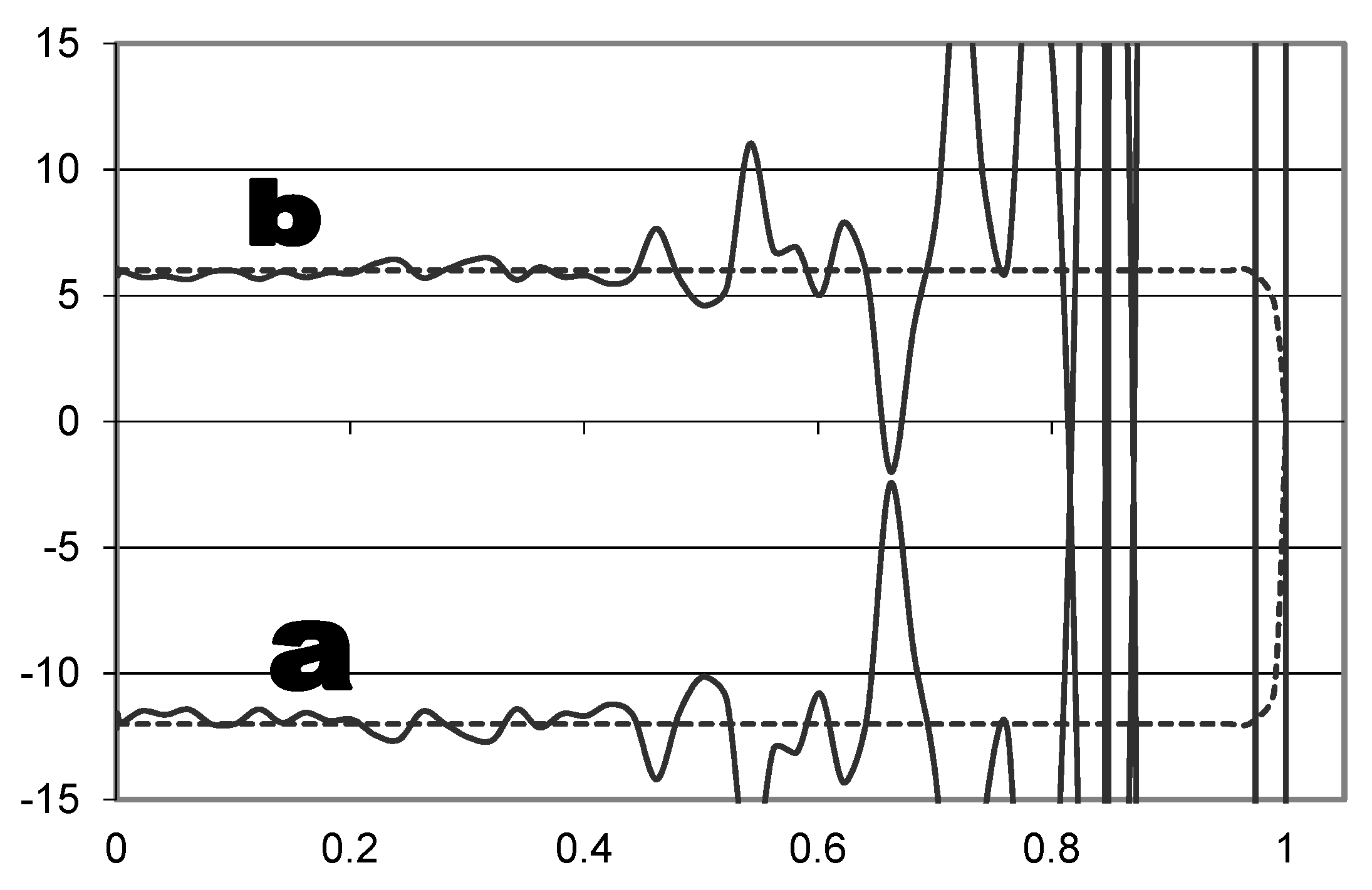
This matrix expression in Equation (24) can be solved in real-time as the simulation progresses in several ways. Two methods are depicted in Figure 3. There is a complication to continuously updating constants a and b. As time approaches the end time (t = 1), the [A] matrix becomes rank deficient, because the rows are linearly dependent. This will cause the computer program to become unstable. The integration constants in Figure 4 vary as time progresses. As t approaches t f = 1 , the values of the constants oscillate unstably to very large values. To account for this shrinking horizon prediction control problem, an optimum open loop controller is inserted and used at these times. We disregard the unstable values that come out of the continuous predictive control logic. Intuition: This should increase cost slightly from the optimum case.
The LU inverse approach to dealing with matrix inverses in Figure 3 required open loop command to occur as early as t = 0.9, while the LU solver approach allows for smaller blind time. This is desirable, because this blind time foreshadows errors in meeting our end conditions. This is a good time to point out that it is not the value of [A]−1. The value of [A]−1 is an intermediate calculation step to get [a b c d]. Calculating the matrix inverse can be problematic, so avoid the unnecessary pitfalls by not calculating [A]−1. Instead, use the LU solver (or QR solver, etc.) or the LU inverse.
This control is somewhat unrealistic, since a body’s onboard computer may not have access to information quickly enough to generate correct integration constants. There is a lag time associated with sensing, and onboard computers may be limited. Accordingly, the next section develops a sampled-data version of this controller, where the sensor data has delayed delivery to the control logic.

2.3. Sampled-Data Predictive Optimum Controller

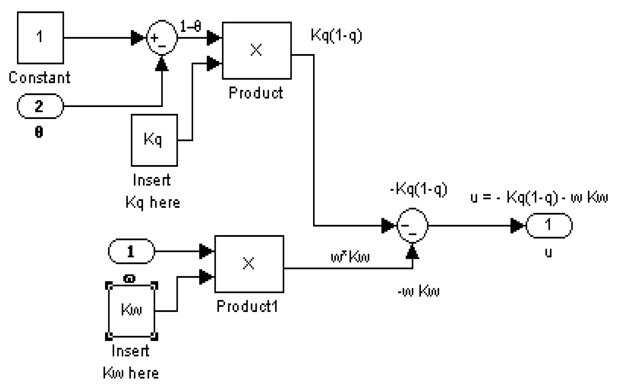
To simulate a real-world sensor delay, a delay was inserted before the control logic in SIMULINK and the delay time was iterated considering acceptable system performance. Using a time delay of 0.05 s allowed this controller to achieve performance in the neighborhood of the other controllers in this study, which establishes the bounds of permissible time lags for performance. Poor Monte Carlo performance required decreasing the time delay to 0.025, while establishing the bounds of permissible time lags for robustness. The letters q and w in the SIMULINK model in Figure 5 are θ and ω, respectively. This is consistent throughout this report.

2.4. Proportional Plus Derivative (PD) Controller Derived Foremost from an Optimization Problem

Defining a = ( K θ + K ω ω ) and b = K θ + K ω ω , the optimum control u = a t + b as a function of the time may be written as a function of states: u = K θ ( 1 t ) + K ω ( 1 t ) ω where the K’s are feedback gains that are functions of the θ and ω error.
The gains could be calculated online, but typically static gains are chosen by the control designer to meet some stated design criteria. This makes the controller performance somewhat arbitrary. For this reason, we can expect non-optimum performance from this controller, unless the stated design criteria comprised only optimization of an identical cost function. In this case, constant PD controller gains were iterated to address the trade-off between low cost and minimum error of stated end conditions. Since gains were iterated via a MATLAB program over a specified range, an applicable descriptive adjective is elusive. The range was finite, so iteration can be done differently by achieving gains (in a range not iterated here).

2.5. Feedforward/Feedback PD Controller

This controller feeds forward (where this topological variant justifies the use of the term “feedforward”) the time-parameterized optimal solution reparametrized as optimal states and then compares the optimum states to the current state to generate the error signal fed to the PD controller, as depicted in Figure 6. The states are taken from a double integrator with the optimum control calculated in Figure 7 corresponding to Equations (19) and (20), as the control logic input seen in Figure 8.

2.6. Two-DOF Controller: Optimal Control Augmented with Feedback Errors Calcuated with Optimal States

Very similar to the previous controller, this controller uses the feedforward/feedback method and further adds another comparison to the optimum case. Once again, allowing this topological variant to justify the use of the term “feedforward,” this controller (again) feeds forward the time-parameterized optimal solution reparametrized as optimal states and then compares the optimum states to the current state to generate the PD feedback portion of the control. Next, the output of the PD controller is also compared to the optimum control in an outer loop context depicted in Figure 9, which permits the optimal (time-parameterized) control to insure good target tracking performance. The optimal control (reparametrized as states) is used for feedback to yield robustness despite not accounting for the deleterious disturbance in a more-complicated problem formulation. The utilization of the results of the optimization problem lead to the terminology “two degree of freedom” or “2DOF” to indicate the two opportunities for the control designer.

3. Results

This section is divided into two portions. The first portion summarizes the simulation analysis of the deterministic plant (the double integrator). The second portion summarizes the simulation analysis of the mismodeled plant (the double integrator with an inertia-velocity control dependence). After succinct display of the results, a detailed discussion follows that summarizes some of the main lessons learned.

3.1. Monte Carlo Analysis on a Deterministic Plant with Noise

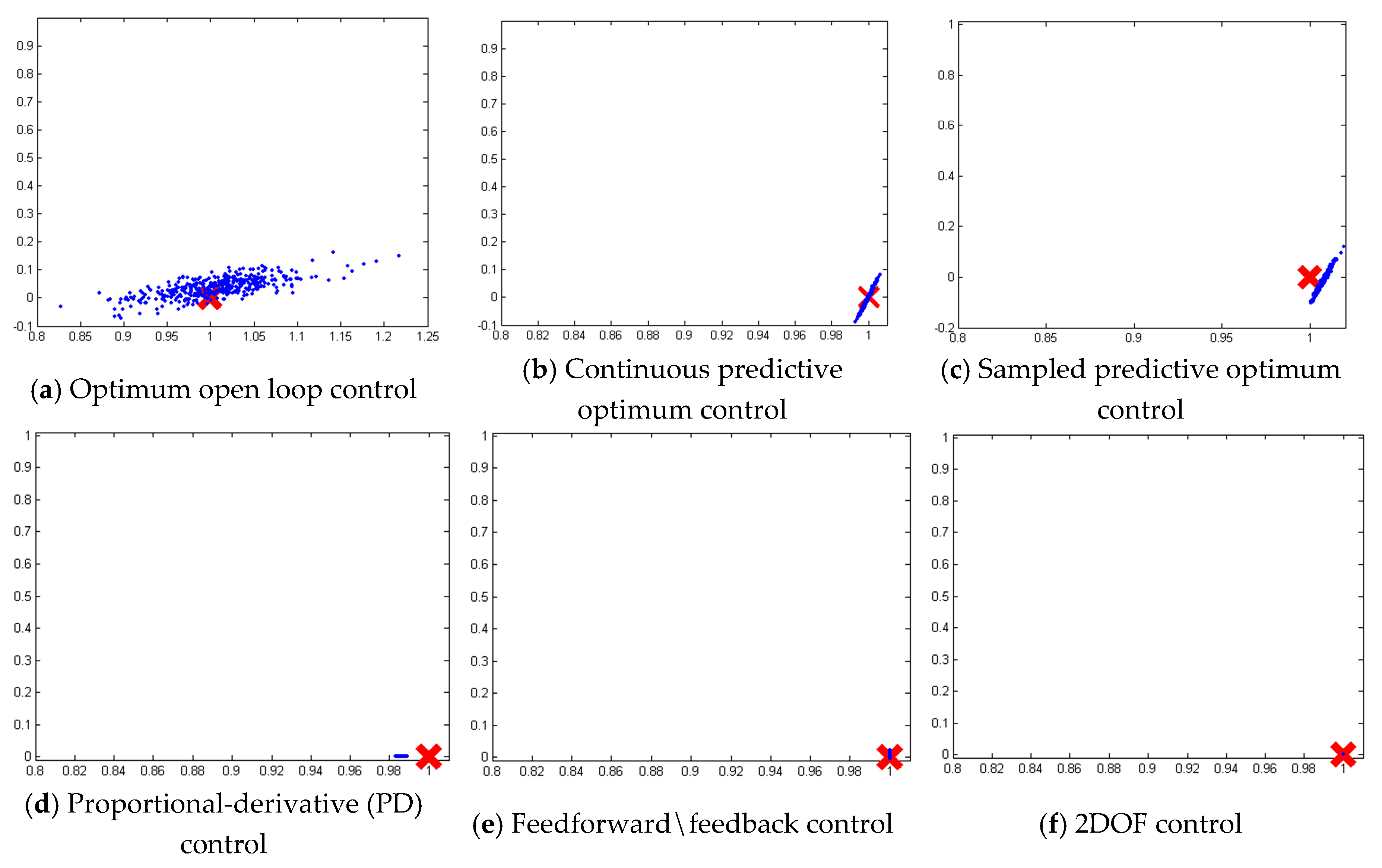
To critically evaluate robustness, random noise was added to the deterministic plant, and identical experiments were simulated from the initial position θ ( 0 ) = 0 to the final position θ ( 1 ) = 1 while ω ( 0 ) = ω ( 1 ) = 0 . Comparison of the controller’s performance is made based on the mean and standard deviations of meeting both the final conditions and also the mean cost displayed in Table 1.

3.2. Open Loop Optimal Controller

First, note the open loop optimum controller. Quickly checking the Appendix A, we see that it optimally achieved the exact end conditions when no noise was present. Everything seemed perfect until we added noise to the plant: +5% inertia noise, +0.1° θ measurement noise, and +0.1 degrees/second ω measurement noise. In the Appendix A, we immediately noticed missed end conditions. The 3σ Monte Carlo analysis allowed the θ, ω and inertia parameters to vary by 0.1, 0.1, and 0.05, respectively. This further antagonized the open loop controller. Note the very large deviation and mean error. Note the cost was below the optimal scalar value of 6. Squashing the enthusiasm seemingly exceeded the mathematically optimal cost. The end conditions were not met precisely. Considering the errors, open loop is not the way to implement optimum control in this case.

3.3. Continuous-Update Optimal Controller

The Continuous Update Optimum Controller seems to have exactly met the stated conditions and minimized the cost without noise. This controller also handles the measurement and inertia noise very well. End conditions are nearly met at a very low cost (nearly optimum). However, the Monte Carlo analysis reveals susceptibility to random errors (especially angular velocity conditions). Mean error and deviation for angular velocity were the third highest of all the controllers recalling the handicap of a blind time. Since a continuously updated optimum controller that calculates its measurement matrix at every instance of time is an idealization, implementation uses a sampled-data computer system. Therefore, the next section examines the Sample Predictive Optimum Controller.

3.4. Sample-Predictive Optimum Controller

The angular position and velocity were sampled at a rate simulating delays in processing and commanding onboard a real body, and the Sampled Predictive Controller performed very well. Selecting a time delay of 0.05 s with no noise, the controller performed very close to optimum levels, and performed modestly well (at least as good as our PD controller to be discussed shortly) in the presence of noise. Monte Carlo analysis revealed the same vulnerability to random conditions seen with the Continuously Updated Controller (particularly susceptible to random angular velocity conditions). The delay time was reduced to 0.025 s to regain a nominal performance. However, its performance mimics the continuously updated case so that we could consider real-world implementation of this controller, if the controller’s application can accept the high angular velocity error and deviation.

3.5. PD Control Derived Foremost from an Optimization Problem

The PD controller does a modest job at achieving the stated end conditions even in the presence of noise, but the cost is huge. As the controller was tuned to more exactly meet the end conditions, cost rose in illustration of the ubiquitous trade-off. The relative immunity to noise foreshadowed its very good performance in the Monte Carlo analysis. The PD controller was not the absolute best controllers regarding θ deviation and mean error. However, it was the best controller when considering ω deviation and mean error. The PD controller does not reveal a susceptibility to random angular velocity conditions that we noted earlier with other controllers. The downside is the cost, which is the highest cost by far. The PD controller design was adjusted to get the nominal cost down to near 30, but the cost sky-rocketed to more than 50 during Monte Carlo analysis. In the next section, the optimum feedforward control will be added to augment the PD controller.

3.6. Feedforward/Feedback PD Controller

Applying the optimum control states to the control logic of our PD controller lead to the Feedforward/Feedback PD Controller, which performed very well. We nearly exactly met the stated end conditions with very low cost. Some susceptibility to noise leads to slightly increased missing of the end conditions and a slightly increased cost (yet remaining far superior to the PD controller). This foreshadows the good performance evident in the random analysis displayed in Figure 10e. The feedforward/feedback controller had the second-best θ deviation and mean error of all the controllers. It showed some modest vulnerability to random errors in ω deviation and error. The significant part is the vastly improved cost. This controller did a very good job meeting end conditions while simultaneously keeping cost pretty low. The next section examines the addition of the optimum control in addition to the optimum states via the 2DOF Controller.

3.7. Two-DOF Controller: Optimal Control Augmented with Feedback Errors Calcuated with Optimal States

The 2DOF controller is another very good controller in the presence of noise (noting a similar increase in cost with the feedforward/feedback controller). In Table 1, the 2DOF controller eliminated the ω deviation and mean error vulnerability to random noise that we saw with the other optimum controllers. The cost was (very slightly) higher than we saw with the feedforward/feedback controller. Using an applicable label from the sport of boxing, this controller may be viewed as the “pound-for-pound” best controller. It essentially matched the #1 performance of the Feedforward/Feedback controller for θ deviation and mean error. Simultaneously, it nearly matched the #1 performance of the PD controller for ω deviation and mean error. All the while, it was also superior regarding cost. If the control requirements can accommodate the slightly higher ω deviation and mean error, the feedforward/feedback controller is best based on lower cost. Otherwise, the 2DOF controller is clearly superior.

3.8. Monte Carlo Analysis on a Mismodeled Plant with Noise

Similar to Section 3.1, this section summarizes the simulation analysis of a mismodeled plant (the double integrator with an inertia-velocity control dependence). In this section, comments are restricted to changes in controller performance due to the mismodeled plant. Generally, the controllers maintained the characteristics demonstrated with the deterministic plant (e.g., the PD controller and the 2 DOF PD controller did not demonstrate susceptibility to ω uncertainty like the other controllers). Applying these controllers to a mismodeled plant, notice in Table 2 that many of the controllers still perform very well (surprising, since the controls were based in optimization of analytic dynamics that were not correct). The controllers experienced slightly degraded performance overall, that, in most cases, was well within expected tolerances for most simple applications.
If the situation demands precise attainment of the final conditions with mismodeled plants, we can deduce four tiers of controllers: (1) 2 DOF PD controller, (2) PD controller and Feedforward/Feedback PD controller, and (3) Continuous, and Sampled Predictive controllers, and (4) Optimal Open Loop Controller. The first tier (the 2DOF PD controller) met the stated end conditions within a miniscule error and maintained a very low-cost number (while not optimum). The second tier (PD and Feedforward/Feedback PD) each did well at meeting one of the stated end conditions, but showed increased error in the other end condition. The third tier (Continuous/Sampled Optimal Controllers) had increased error in both stated end conditions, while the final tier (the open loop controller) was inappropriate for application due to high errors and deviation in end conditions.
If the requirements on stated end conditions can be relaxed sufficiently to emphasize minimum cost, the tiers of results would change. The optimum open loop controller would join the first tier due to its minimum cost, but such a re-ranking will not be done in this case due to the large error achieving end conditions. The first tier would include the continuous and the sample optimum controllers. They achieved minimum cost while also closely meeting the end conditions. Next, the second tier would include feedback/feedforward and 2DOF PD controllers. They had slightly higher costs while very precisely meeting the stated end conditions. Third, the PD controller had very high cost, but also did a good job meeting the end conditions.

4. Discussion

Predictive controllers (both continuous and sampled-data) derived from the outset to be optimal by first solving an optimization problem with the governing dynamic equations of motion lead to several controllers (including a controller that twice invokes optimization to formulate robust, predictive control, which was referred to as a two degree-of-freedom controller). These controllers were compared to each other with noise and modeling errors in Table 3. Many figures of merit are used: tracking error and rate error deviations and means, in addition to total mean cost. Robustness was evaluated using Monte Carlo analysis where plant parameters were randomly assumed to be incorrectly modeled. Six instances of controllers were compared against these methods and interpretations allow engineers to select a tailored control for their given circumstances. Optimal control, predictive control, discrete (sampled-data) control, proportional-derivative control, feedforward + feedback control, and a proposed 2DOF control were all derived with the articulation of an individual optimization problem. Control structures were then designed to enforce optimality, rather than the ubiquitous methodology of first asserting the control structure, then subsequently seeking to optimize the imposed structure. The proposed comparison paradigm utilized six disparate types of control that were compared against each other’s ability to meet commanded end conditions at minimum cost in the face of both noise and modeling errors.
The optimal open loop controller established the baseline cost (being the mathematical minimum possible), but was not realistically capable of implementation due to lacking feedback. Continuous and discrete (sampled-data) predictive controls proved very good at achieving the commanded final position with very low cost, but revealed a tolerable, but non-trivial, susceptibility to noise and mismodeling only with regard to difficulties achieving the final commanded velocity state. Very much akin the classical PD controller, the proportional-derivative controller developed under the new design paradigm was very good at state control (achieving the best rate control), but had the highest cost by a very wide margin compared to all of the other control options. Akin to classical feedforward + feedback controllers, the controller designed under the new paradigm achieved the very best position control at very good cost. However, it has some slight susceptibility to noise and modeling errors with regard to the rate control. The proposed 2DOF controller was the all-around best controller, achieving near-perfect state controls with very low (suboptimal) cost. The controller had no performance degradation due to noise or modeling errors.
Proposed 2DOF control designed foremost as an optimization problem: The open-loop optimal control is used as a feedforward, while the optimal states derived from a time-parameterized optimal control are compared to the feedback signal to generate the error fed to the feedback controller whose gains are a reparameterization of the optimal solution.

5. Future Works

Noise was not treated in the problem formulation, but the proposed 2DOF controller achieved near-precision accuracy with near-minimal costs in the face of noise. It remains of interest to investigate whether further performance improvement is possible by augmenting the problem formulation with smooth filters (e.g., Kalman filters). Since target tracking accuracy was near machine-precision even with modeling errors and noise, the investigation of smoothing filters should seek to further reduce the already low-cost value.

Funding

This research received no external funding.

Acknowledgments

Timothy Sands is not a tenured faculty member of Columbia University. Rather, he is the Associate Dean of the Naval Postgraduate School’s Graduate School of Engineering and Applied Sciences. In order to avoid legal jeopardy, Timothy Sands publishes government-funded research under his association with the Naval Postgraduate School, while publishing non-government funded research under his continuing associations with Stanford and Columbia Universities.

Conflicts of Interest

The author declares no conflict of interest.

Appendix A

The appendix contains detailed explanations of experimental details that would disrupt the flow of the main text, but, nonetheless, remain crucial to understanding and reproducing the research shown. It contains figures of replicates for simulation experiments of which representative data is shown in the main text. For each of the controllers implemented, figures of the SIMULINK models used to generate the results are provided and summarized in this research report. Each system was tested with no noise and then with a +1% angle and rate sensor noise and 5% body inertia noise. Each system was compared to the optimum open loop controller (with no noise) via l2 error norms.

Appendix A.1. Optimum Open Loop Controller-No Noise
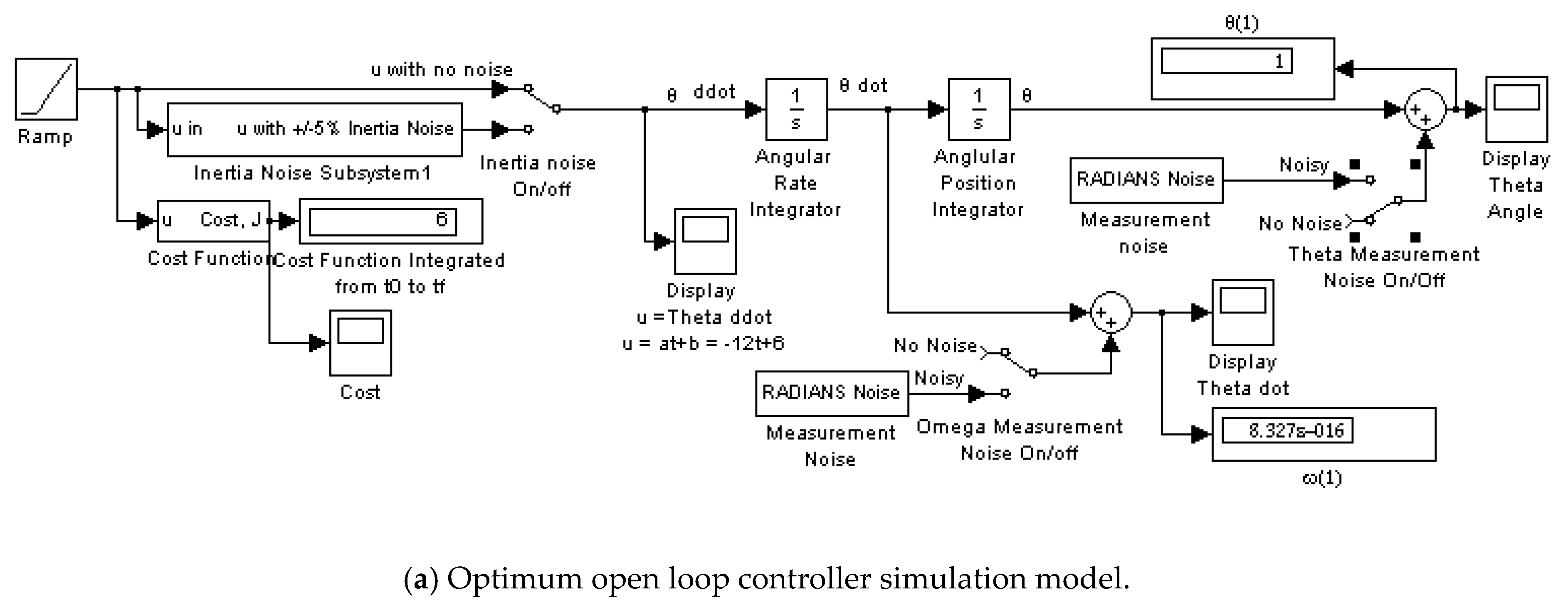
Figure A1. Optimum open loop controller simulation model and results.
Algorithms 12 00232 g0a1aAlgorithms 12 00232 g0a1b

Appendix A.2. Optimum Open Loop Controller-with Noise
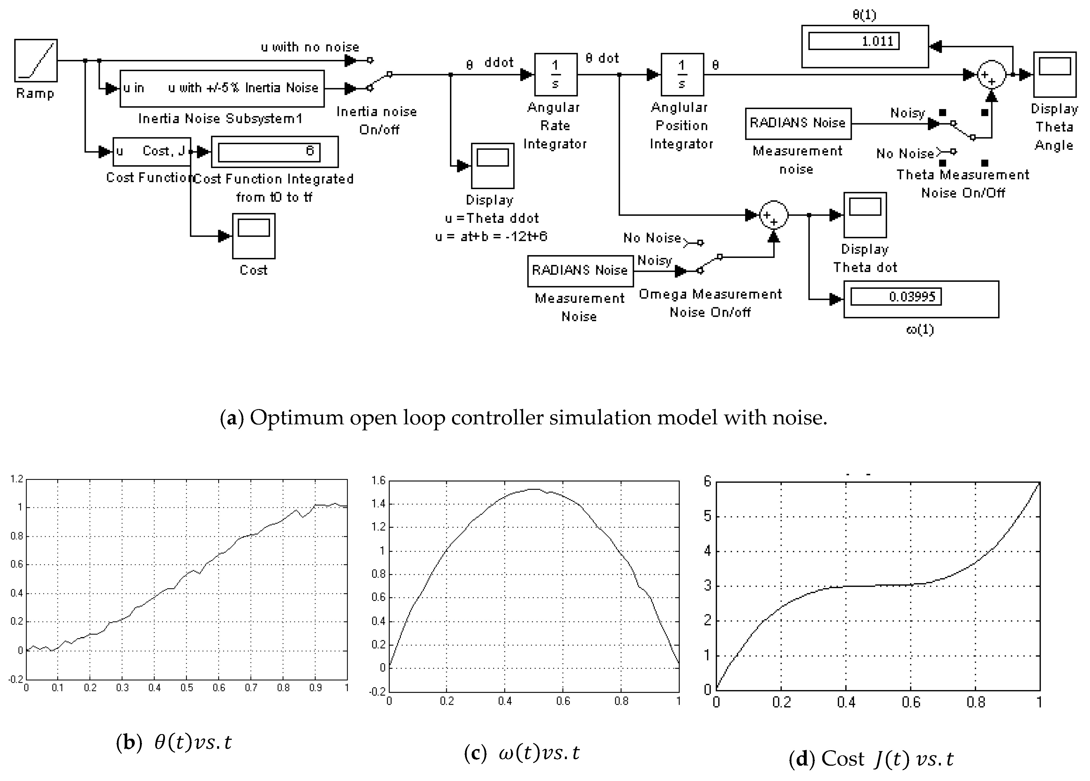
Figure A2. Optimum open loop controller simulation model with noise and results.
Algorithms 12 00232 g0a2

Appendix A.3. PD Controller No Noise

Figure A3. Proportional-derivative (PD) controller ( K w = 13.3 ,   K q = 40 ) simulation model.
Algorithms 12 00232 g0a3

Appendix A.4. PD Controller with Noise
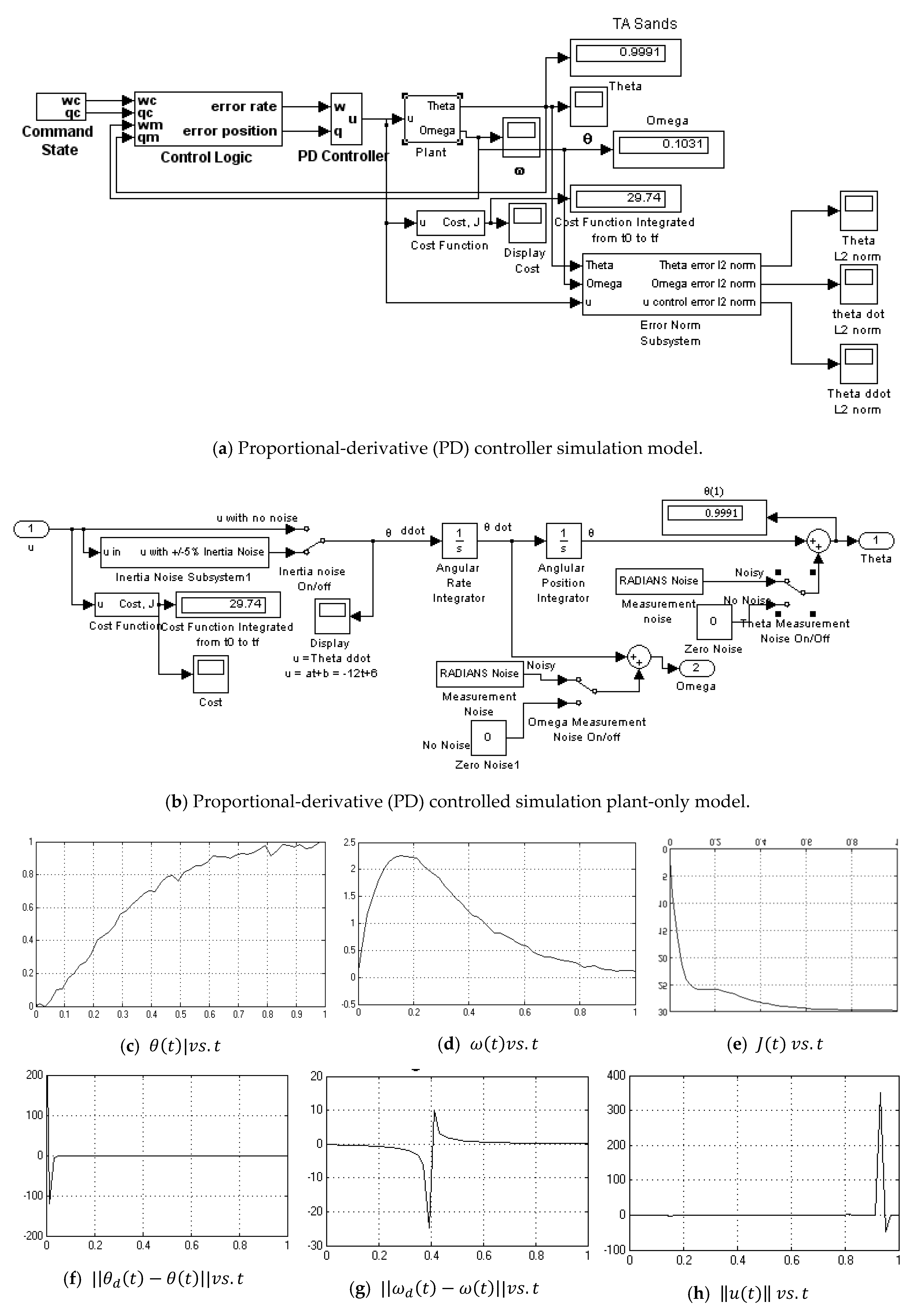
Figure A4. Proportional-derivative (PD) controller ( K w = 13.3 ,   K q = 40 ) simulation model with noise.
Algorithms 12 00232 g0a4

Appendix A.5. Continuouse Predictive Optimum Controller-No Noise
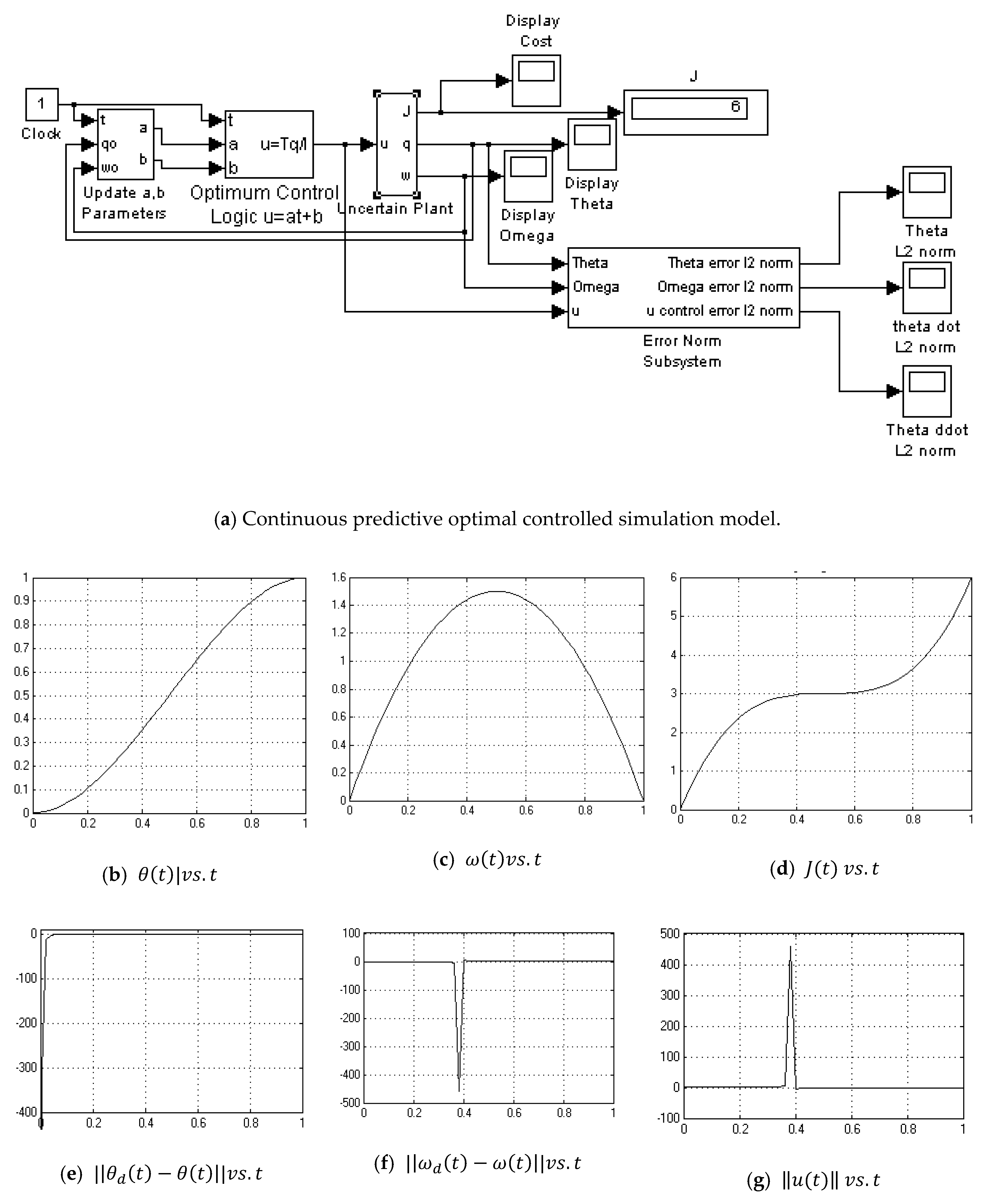
Figure A5. Continuous predictive optimum controlled simulation model.
Algorithms 12 00232 g0a5

Appendix A.6. Continuouse Predictive Optimum Controlle-with Noise
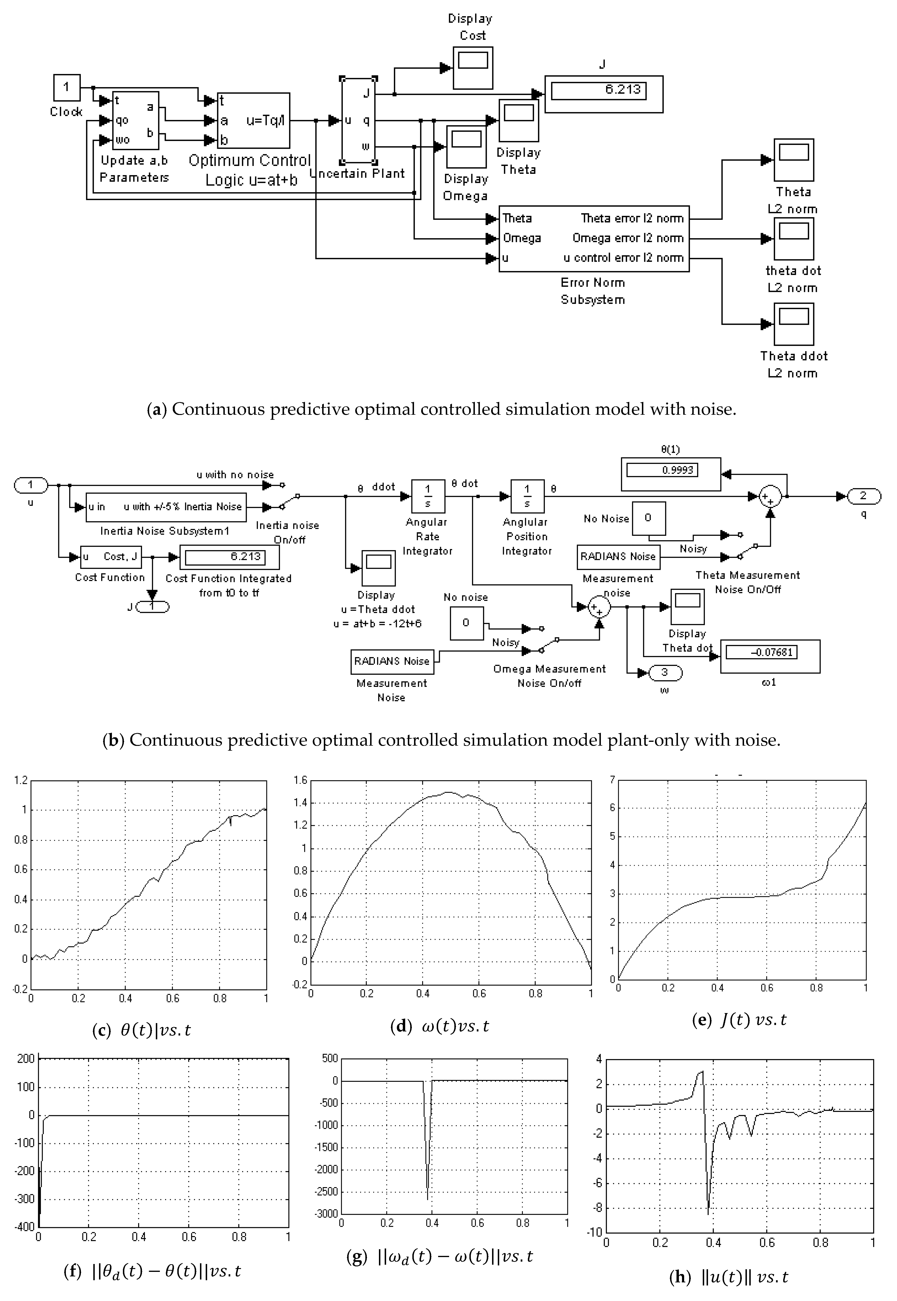
Figure A6. Continuous predictive optimum controlled simulation model with noise.
Algorithms 12 00232 g0a6

Appendix A.7. Feedforward/Feedback PD Controller-No Noise
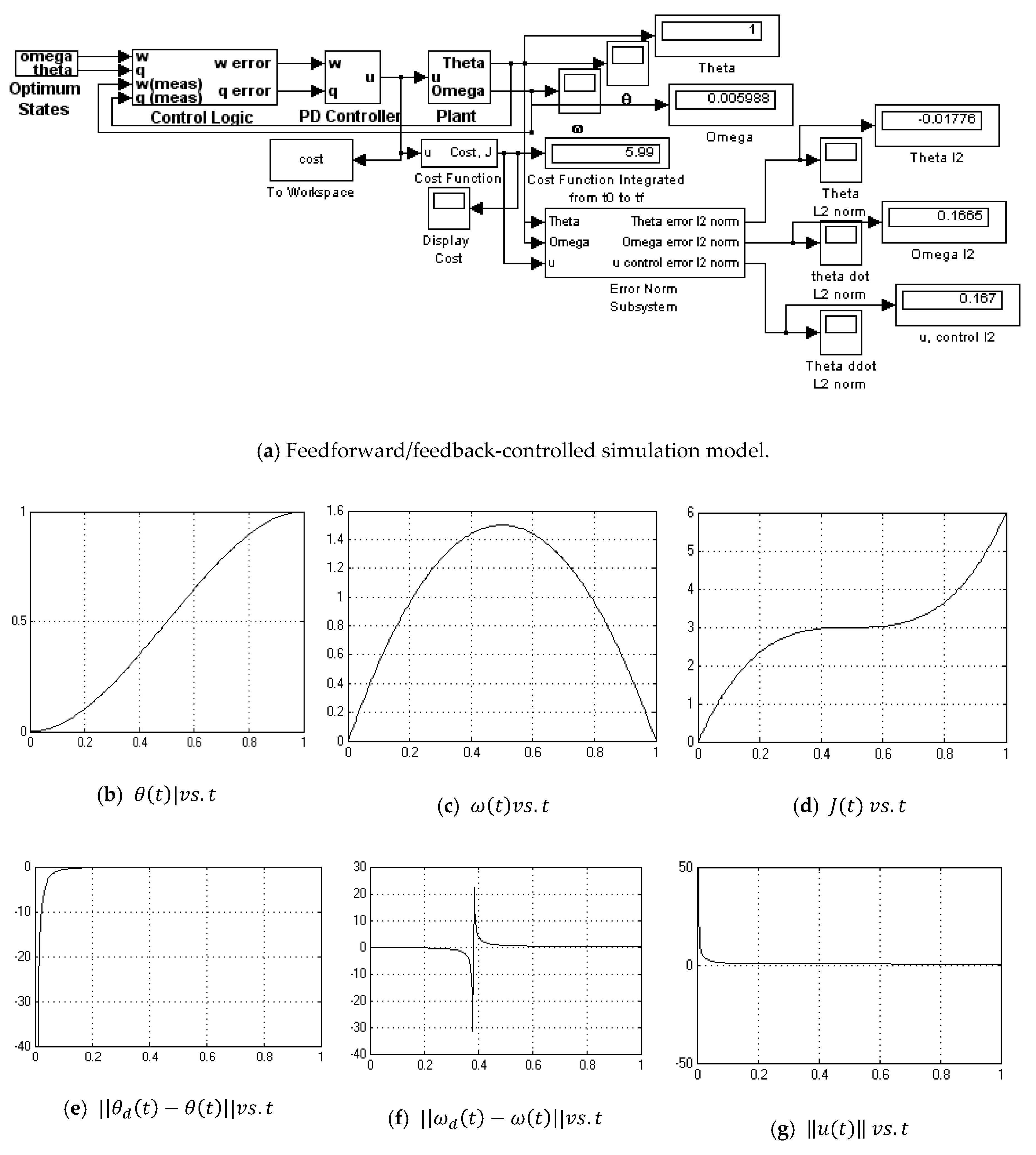
Figure A7. Feedforward/feedback PD controlled simulation.
Algorithms 12 00232 g0a7

Appendix A.8. Feedforward/Feedback PD Controlle-with Noise
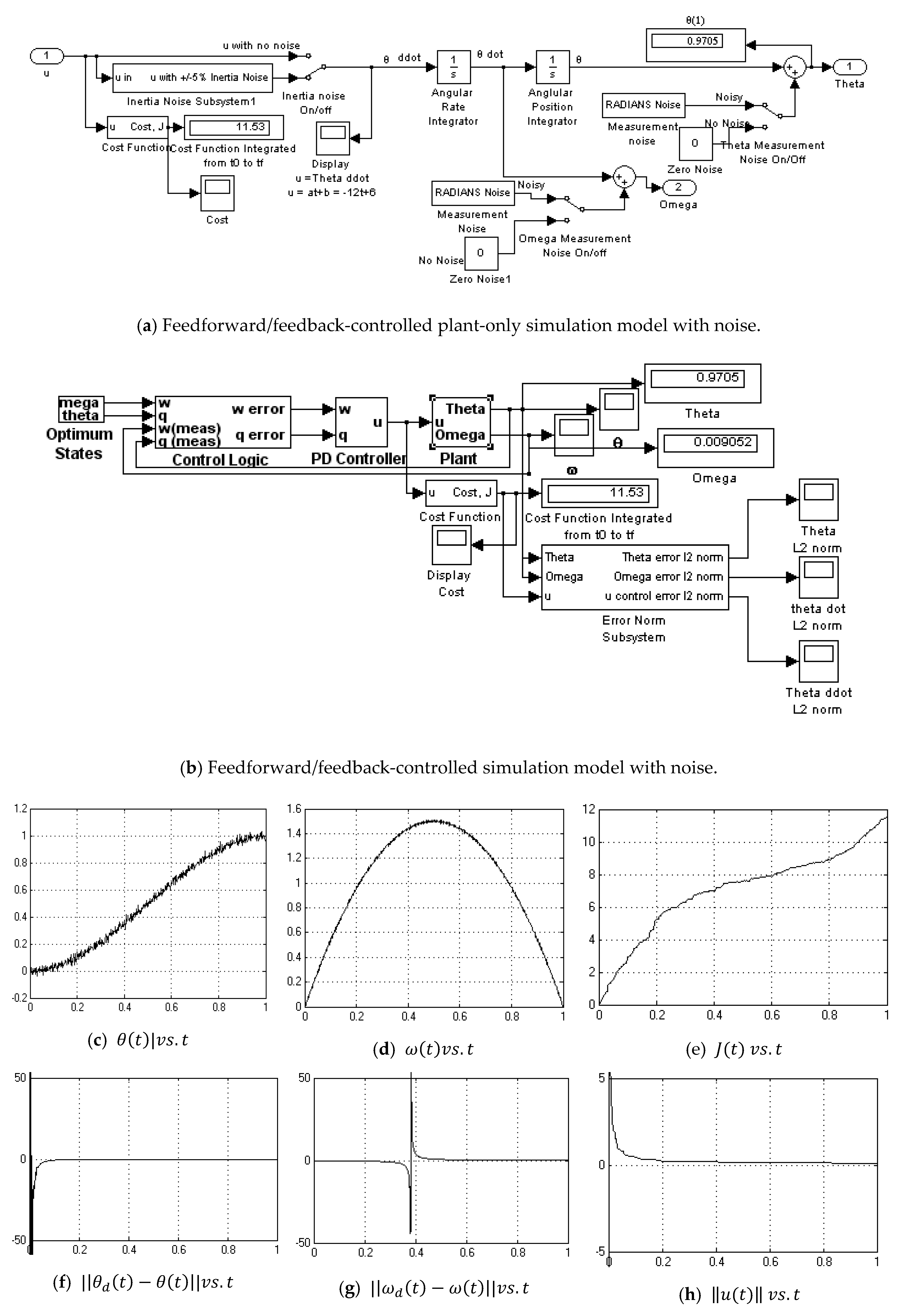
Figure A8. Feedforward/feedback PD controlled simulation with noise.
Algorithms 12 00232 g0a8

Appendix A.9. 2DOF PD Controller-No Noise
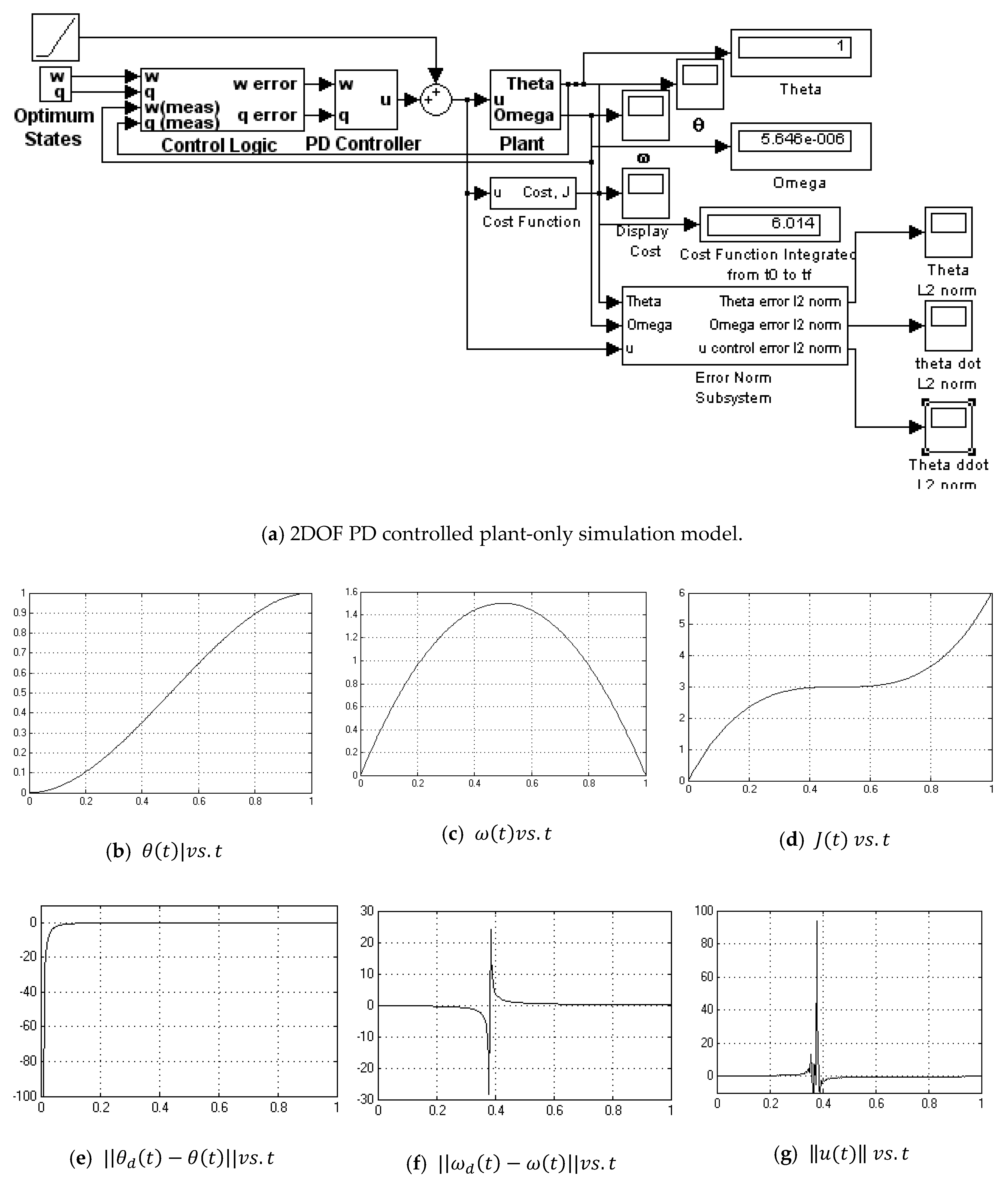
Figure A9. 2DOF PD controlled simulation.
Algorithms 12 00232 g0a9

Appendix A.10. 2DOF PD Controller-with Noise
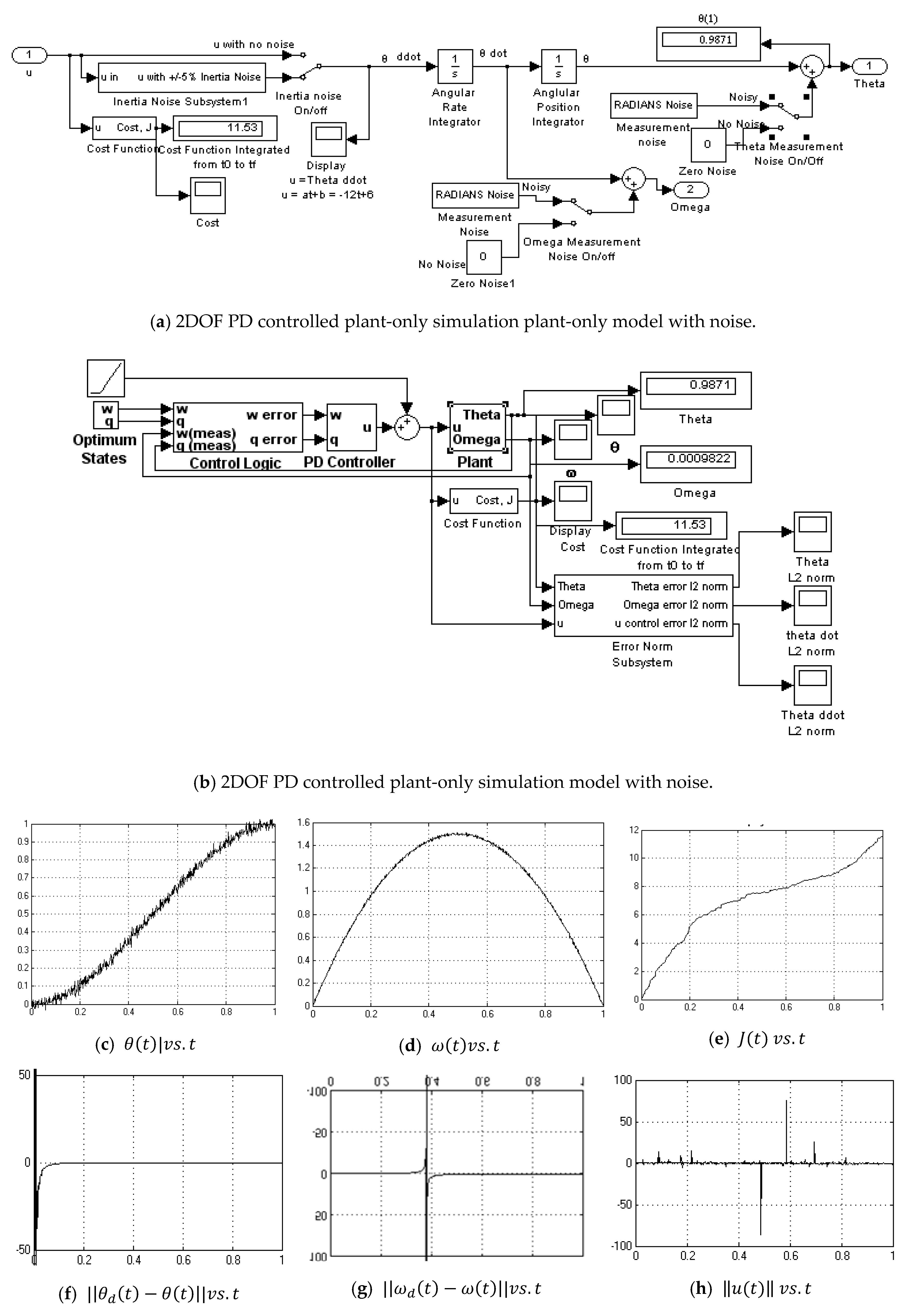
Figure A10. 2DOF PD controlled simulation with noise.
Algorithms 12 00232 g0a10

Appendix A.11. Sampled Predictive Controller-without Noise
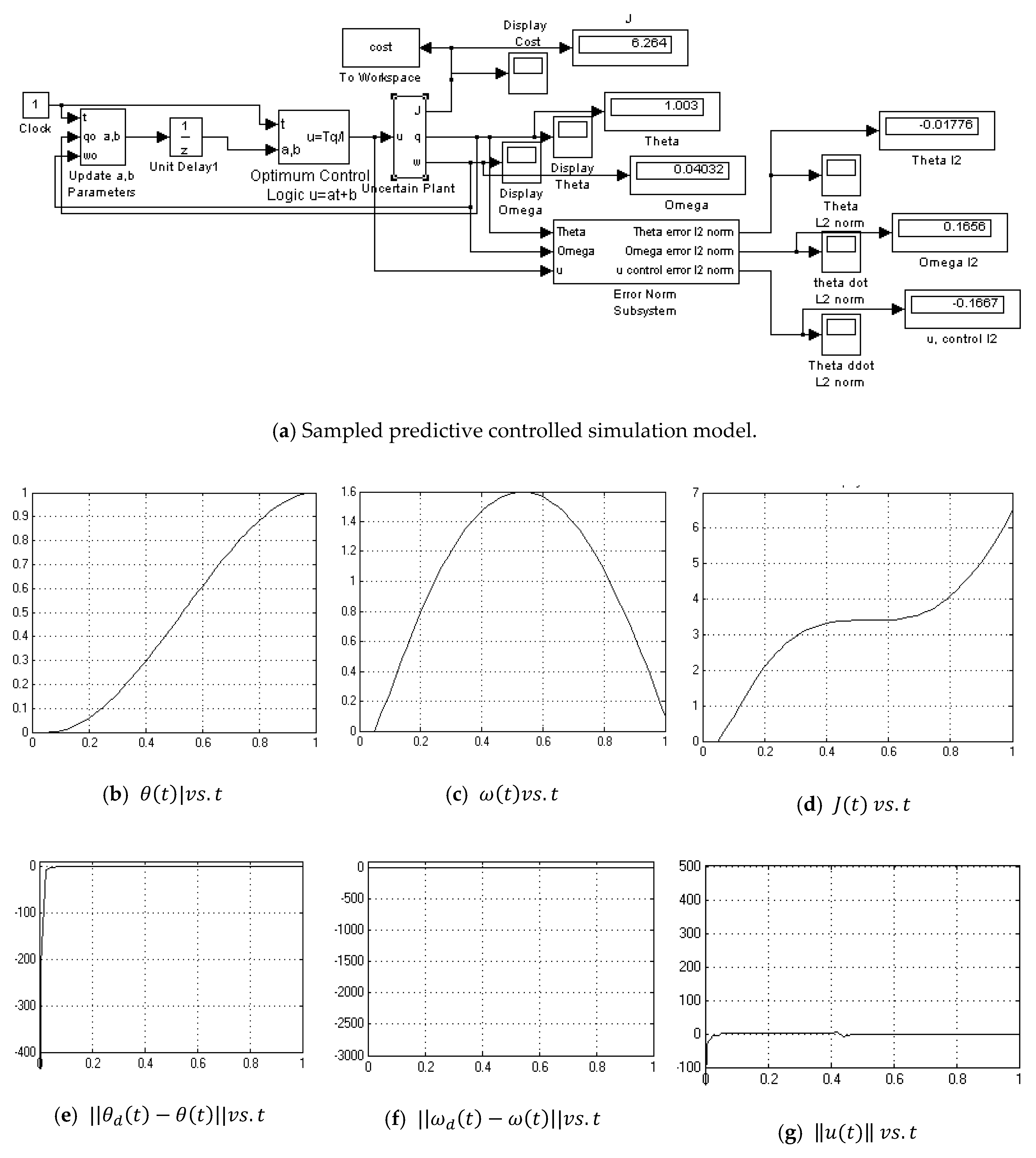
Figure A11. Sampled predictive controlled simulation.
Algorithms 12 00232 g0a11

Appendix A.12. Sampled Predictive Controller-with Noise
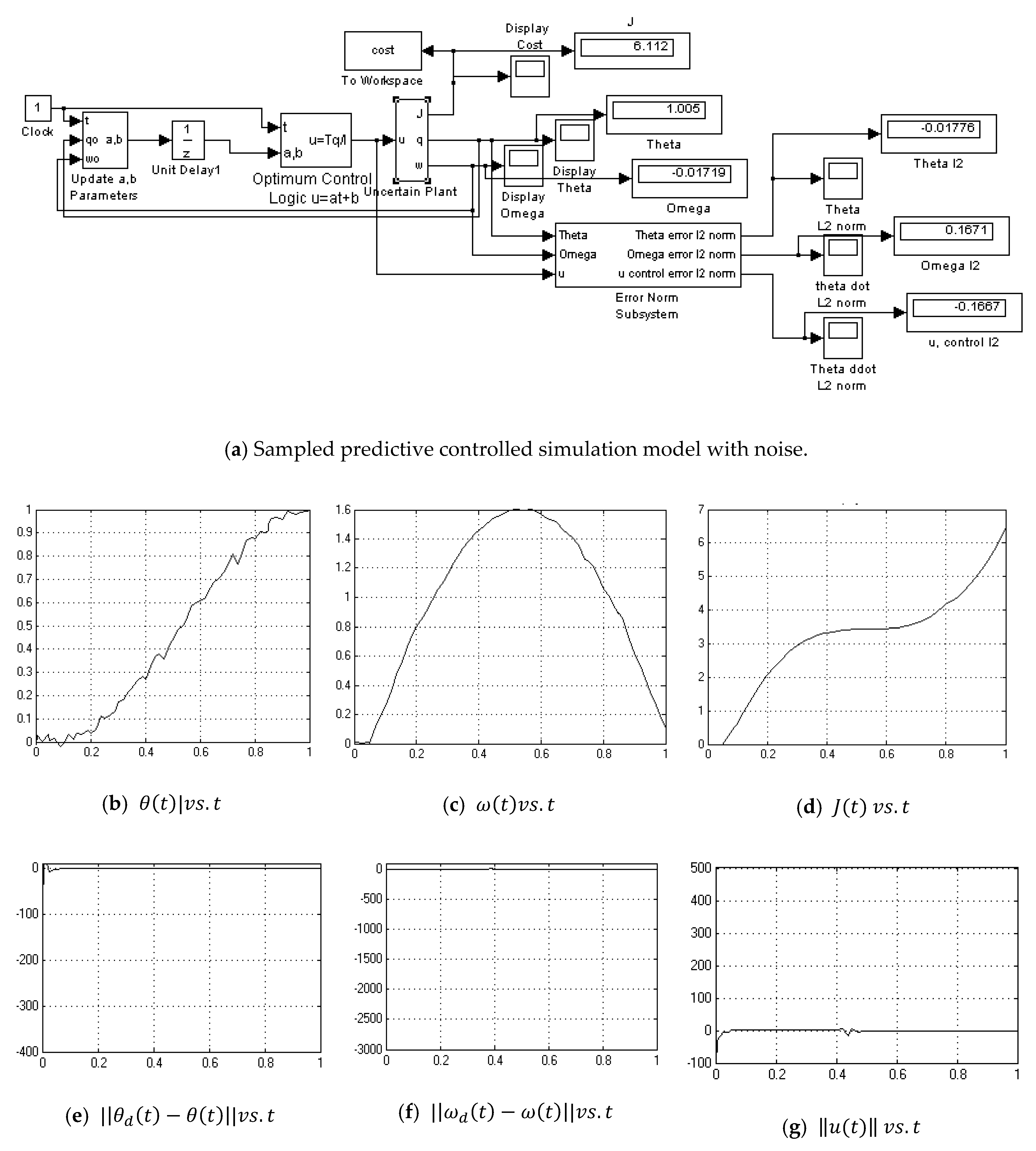
Figure A12. Sampled predictive controlled simulation with noise.
Algorithms 12 00232 g0a12

Appendix A.13. Mismodeled Plant

Figure A13. Mismodeled plant inserted into previous programming.
Algorithms 12 00232 g0a13

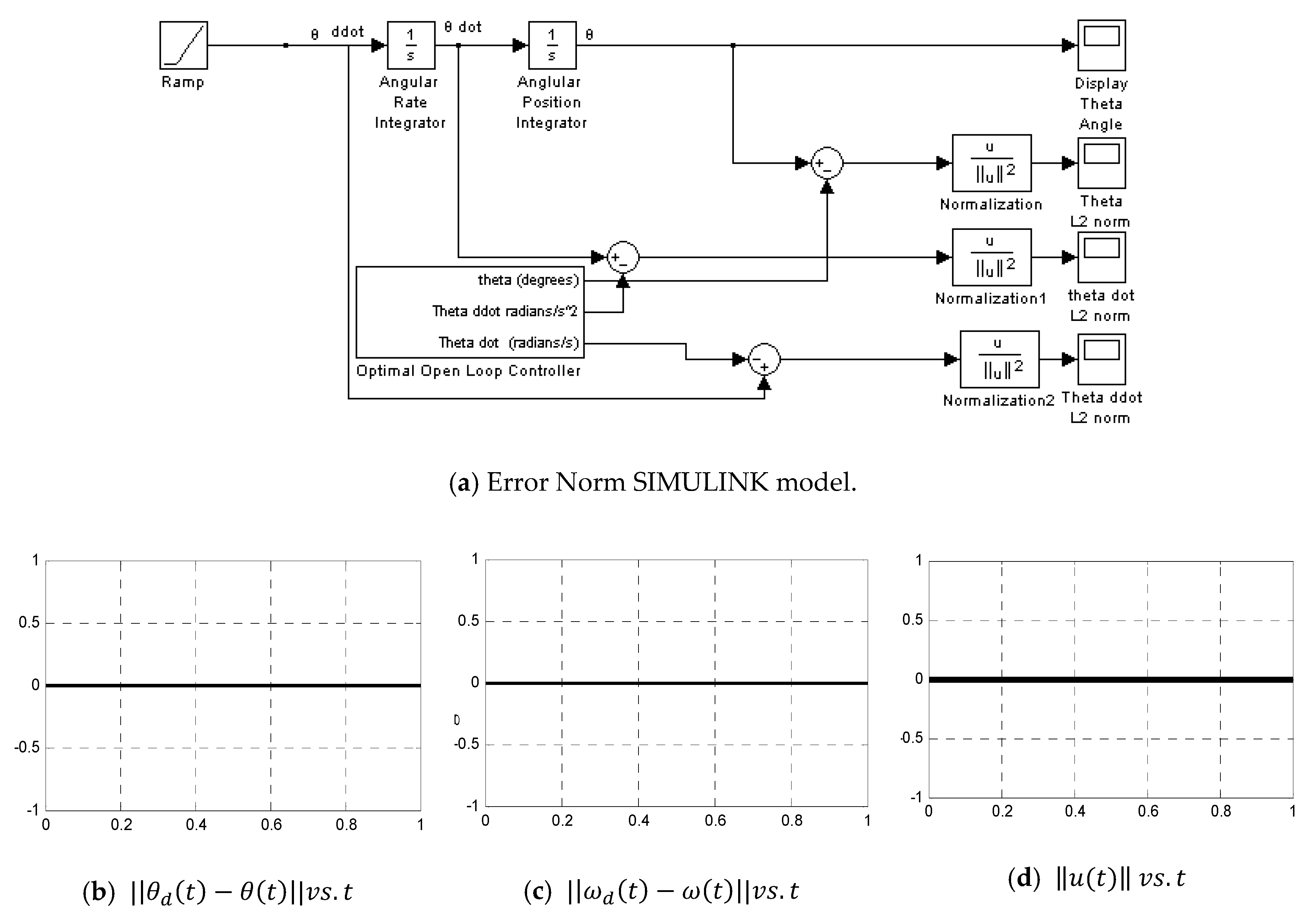
Appendix A.14. Error Norms

Figure A14. Error norm for optimum controller ( 2 = 0 when compared to itself).
Algorithms 12 00232 g0a14

References

  1. Chasles, M. Note sur les propriétés générales du système de deux corps semblables entr’eux. Bull. Sci. Math. Astron. Phys. Chem. 1830, 14, 321–326. (In French) [Google Scholar]
  2. Euler, L. Formulae Generales pro Translatione Quacunque Corporum Rigidorum (General Formulas for the Translation of Arbitrary Rigid Bodies. Novi Comment. Acad. Sci. Petropolitanae 1776, 20, 189–207. Available online: https://math.dartmouth.edu/~euler/docs/originals/E478.pdf (accessed on 2 November 2019).
  3. Newton, I. Principia, Jussu Societatis Regiæ ac Typis Joseph Streater; Cambridge University Library: London, UK, 1687. [Google Scholar]
  4. Turner, A.J. The Time Museum. I: Time Measuring Instruments; Part 3: Water-Clocks, Sand-Glasses, Fire-Clocks; The Museum: Rockford, IL, USA, 1984; ISBN 0-912947-01-2. [Google Scholar]
  5. Lewis, F.L. Applied Optimal Control and Estimation; Prentice-Hall: Upper Saddle River, NJ, USA, 1992. [Google Scholar]
  6. Raol, J.; Ayyagari, R. Control Systems: Classical, Modern, and AI-Based Approaches; CRC Press, Taylor and Francis: Boca Raton, FL, USA, 2020. [Google Scholar]
  7. Wiener, N. Extrapolation, Interpolation, and Smoothing of Stationary Time Series; Wiley: New York, NY, USA, 1949; ISBN 978-0-262-73005-1. [Google Scholar]
  8. Bellman, R.E. Dynamic Programming; Princeton University Press: Princeton, NJ, USA, 1957; ISBN 0-486-42809-5. [Google Scholar]
  9. Pontryagin, L.S.; Boltyanskii, V.G.; Gamkrelidze, R.V.; Mischenko, E.F. The Mathematical Theory of Optimal Processes; Neustadt, L.W., Ed.; Wiley: New York, NY, USA, 1962. [Google Scholar]
  10. Ross, I.M. A Primer on Pontryagin’s Principle in Optimal Control, 2nd ed.; Collegiate Publishers: London, UK, 2015. [Google Scholar]
  11. Kalman, R.E. A New Approach to Linear Filtering and Prediction Problems. J. Basic Eng. 1960, 82, 35. [Google Scholar] [CrossRef]
  12. Anderson, B.D.O.; Moore, J.B. Optimal Control—Linear Quadratic Methods; Prentice-Hall: Upper Saddle River, NJ, USA, 1989. [Google Scholar]
  13. Astrom, K.J.; Bjorn Wittenmark, B. Adaptive Control, 2nd ed.; Prentice-Hall: Upper Saddle River, NJ, USA, 1994. [Google Scholar]
  14. Slotine, J.J.; Weiping Li, W. Applied Nonlinear Control; Pearson: London, UK, 1991. [Google Scholar]
  15. Fossen, T.I. Comments on Hamiltonian Adaptive Control of Spacecraft. IEEE Trans. Autom. Control 1993, 38, 671–672. [Google Scholar] [CrossRef]
  16. Sands, T.; Kim, J.J.; Agrawal, B. Improved Hamiltonian adaptive control of spacecraft. In Proceedings of the Aerospace Conference, Big Sky, MT, USA, 7–14 March 2009; pp. 1–10. [Google Scholar]
  17. Sands, T. Fine Pointing of Military Spacecraft; Naval Postgraduate School: Monterey, CA, USA, 2007. [Google Scholar]
  18. Sands, T. Physics-Based Control Methods, Chapter 2, in Advances in Spacecraft Systems and Orbit Determination; InTechOpen: London, UK, 2012. [Google Scholar]
  19. Sands, T.; Kim, J.J.; Agrawal, B. Spacecraft Adaptive Control Evaluation; Infotech@Aerospace: San Juan, Puerto Rico, 2012. [Google Scholar]
  20. Sands, T. Improved magnetic levitation via online disturbance decoupling. Phys. J. 2015, 1, 272–280. [Google Scholar]
  21. Sands, T.; Armani, C. Analysis, correlation, and estimation for control of material properties. J. Mech. Eng. Autom. 2018, 8, 7–31. [Google Scholar]
  22. Lobo, K.; Lang, J.; Starks, A.; Sands, T. Analysis of deterministic artificial intelligence for inertia modifications and orbital disturbances. Int. J. Control Sci. Eng. 2018, 8, 53–62. [Google Scholar]
  23. Nakatani, S.; Sands, T. Simulation of spacecraft damage tolerance and adaptive controls. In Proceedings of the Aerospace, Big Sky, MT, USA, 1–8 March 2014; pp. 1–16. [Google Scholar]
  24. Nakatani, S.; Sands, T. Autonomous damage recovery in space. Int. J. Autom. Control Intell. Syst. 2016, 2, 23–36. [Google Scholar]
  25. Sands, T. Nonlinear-Adaptive mathematical system identification. Computation 2017, 5, 47. [Google Scholar] [CrossRef]
  26. Cooper, M.; Heidlauf, P.; Sands, T. Controlling chaos—Forced van der pol equation. Mathematics 2017, 5, 70. [Google Scholar] [CrossRef]
  27. Sands, T. Space system identification algorithms. J. Space Explor. 2017, 6, 138. [Google Scholar]
  28. Sands, T. Phase lag elimination at all frequencies for full state estimation of spacecraft attitude. Phys. J. 2017, 3, 1–12. [Google Scholar]
  29. Nakatani, S.; Sands, T. Battle-Damage tolerant automatic controls. Electr. Electron. Eng. 2018, 8, 23. [Google Scholar]
  30. Baker, K.; Cooper, M.; Heidlauf, P.; Sands, T. Autonomous trajectory generation for deterministic artificial intelligence. Electr. Electron. Eng. 2018, 8, 59–68. [Google Scholar]
  31. Sands, T.; Bollino, K. Autonomous Underwater Vehicle Guidance, Navigation, and Control, chapter in Autonomous Vehicles; InTechOpen: London, UK, 2018; Available online: https://www.intechopen.com/online-first/autonomous-underwater-vehicle-guidance-navigation-and-control (accessed on 2 November 2019). [CrossRef]
  32. Sands, T.; Bollino, K.; Kaminer, I.; Healey, A. Autonomous Minimum Safe Distance Maintenance from Submersed Obstacles in Ocean Currents. J. Mar. Sci. Eng. 2018, 6, 98. [Google Scholar] [CrossRef]
  33. Sidhu, H.S.; Siddhamshetty, P.; Kwon, J.S. Approximate Dynamic Programming Based Control of Proppant Concentration in Hydraulic Fracturing. Mathematics 2018, 6, 132. [Google Scholar] [CrossRef]
  34. Gao, S.; Zheng, Y.; Li, S. Enhancing Strong Neighbor-Based Optimization for Distributed Model Predictive Control Systems. Mathematics 2018, 6, 86. [Google Scholar] [CrossRef]
  35. Zhang, X.; Wang, R.; Bao, J. A Novel Distributed Economic Model Predictive Control Approach for Building Air-Conditioning Systems in Microgrids. Mathematics 2018, 6, 60. [Google Scholar] [CrossRef]
  36. Xue, D.; El-Farra, N.H. Forecast-Triggered Model Predictive Control of Constrained Nonlinear Processes with Control Actuator Faults. Mathematics 2018, 6, 104. [Google Scholar] [CrossRef]
  37. Wong, W.C.; Chee, E.; Li, J.; Wang, X. Recurrent Neural Network-Based Model Predictive Control for Continuous Pharmaceutical Manufacturing. Mathematics 2018, 6, 242. [Google Scholar] [CrossRef]
  38. Sands, T.; Kenny, T. Experimental piezoelectric system identification. J. Mech. Eng. Autom. 2017, 7, 179–195. [Google Scholar]
  39. Sands, T. Deterministic Artificial Intelligence; InTechOpen: London, UK, 2019; ISBN 978-1-78984-111-4. [Google Scholar]
  40. Sands, T. Optimization Provenance of Whiplash Compensation for Flexible Space Robotics. Aerospace 2019, 6, 93. [Google Scholar] [CrossRef]
  41. Lee, J.H.; Ricker, N.L. Extended Kalman Filter Based Nonlinear Model Predictive Control. In Proceedings of the American Control Conference, San Francisco, CA, USA, 2–4 June 1993. [Google Scholar]
  42. Wang, C.; Ohsumi, A.; Djurovic, I. Model Predictive Control of Noisy Plants Using Kalman Predictor and Filter. In Proceedings of the IEEE TECON, Beijing, China, 28–31 October 2002. [Google Scholar]
  43. Sørensenog, K.; Kristiansen, S. Model Predictive Control for an Artificial Pancreas. Bachelor’s Thesis, Technical University of Denmark, Lyngby, Denmark, 2007. [Google Scholar]
  44. Huang, R.; Patwardhan, S.C.; Biegler, L.T. Robust stability of nonlinear model predictive control with extended Kalman filter and target setting. Int. J. Rob. Nonlinear Control 2012, 23, 1240–1264. [Google Scholar] [CrossRef]
  45. Hong, M.; Cheng, S. Model Predictive Control Based on Kalman Filter for Constrained Hammerstein-Wiener Systems. Math. Probl. Eng. 2013, 6, 2013. [Google Scholar] [CrossRef]
  46. Ikonen, E. Model Predictive Control and State Estimation; University of Oulu: Oulu, Finland, 2013; Available online: http://cc.oulu.fi/~iko/SSKM/SSKM2016-MPC-SE.pdf (accessed on 2 November 2019).
  47. Binette, J.-C.; Srinivasan, B. On the Use of Nonlinear Model Predictive Control without Parameter Adaptation for Batch Processes. Processes 2016, 4, 27. [Google Scholar] [CrossRef]
  48. Cao, Y.; Kang, J.; Nagy, Z.K.; Laird, C.D. Parallel Solution of Robust Nonlinear Model Predictive Control Problems in Batch Crystallization. Processes 2016, 4, 20. [Google Scholar] [CrossRef]
  49. Ganesh, H.S.; Edgar, T.F.; Baldea, M. Model Predictive Control of the Exit Part Temperature for an Austenitization Furnace. Processes 2016, 4, 53. [Google Scholar] [CrossRef]
  50. Jost, F.; Sager, S.; Le, T.T.-T. A Feedback Optimal Control Algorithm with Optimal Measurement Time Points. Processes 2017, 5, 10. [Google Scholar] [CrossRef]
  51. Xu, K.; Timmermann, J.; Trächtler, A. Nonlinear Model Predictive Control with Discrete Mechanics and Optimal Control. In Proceedings of the IEEE International Conference on Advanced Intelligent Mechatronics (AIM), Munich, Germany, 3–7 July 2017. [Google Scholar]
  52. Suwartadi, E.; Kungurtsev, V.; Jäschke, J. Sensitivity-Based Economic NMPC with a Path-Following Approach. Processes 2017, 5, 8. [Google Scholar] [CrossRef]
  53. Vaccari, M.; Pannocchia, G. A Modifier-Adaptation Strategy towards Offset-Free Economic MPC. Processes 2017, 5, 2. [Google Scholar] [CrossRef]
  54. Kheradmandi, M.; Mhaskar, P. Data Driven Economic Model Predictive Control. Mathematics 2018, 6, 51. [Google Scholar] [CrossRef]
  55. Durand, H. A Nonlinear Systems Framework for Cyberattack Prevention for Chemical Process Control Systems. Mathematics 2018, 6, 169. [Google Scholar] [CrossRef]
  56. Tian, Y.; Luan, X.; Liu, F.; Dubljevic, S. Model Predictive Control of Mineral Column Flotation Process. Mathematics 2018, 6, 100. [Google Scholar] [CrossRef]
  57. Wu, Z.; Durand, H.; Christofides, P.D. Safeness Index-Based Economic Model Predictive Control of Stochastic Nonlinear Systems. Mathematics 2018, 6, 69. [Google Scholar] [CrossRef]
  58. Liu, S.; Liu, J. Economic Model Predictive Control with Zone Tracking. Mathematics 2018, 6, 65. [Google Scholar] [CrossRef]
  59. Bonfitto, A.; Castellanos Molina, L.M.; Tonoli, A.; Amati, N. Offset-Free Model Predictive Control for Active Magnetic Bearing Systems. Actuators 2018, 7, 46. [Google Scholar] [CrossRef]
  60. Godina, R.; Rodrigues, E.M.G.; Pouresmaeil, E.; Matias, J.C.O.; Catalão, J.P.S. Model Predictive Control Home Energy Management and Optimization Strategy with Demand Response. Appl. Sci. 2018, 8, 408. [Google Scholar] [CrossRef]
  61. Khan, H.S.; Aamir, M.; Ali, M.; Waqar, A.; Ali, S.U.; Imtiaz, J. Finite Control Set Model Predictive Control for Parallel Connected Online UPS System under Unbalanced and Nonlinear Loads. Energies 2019, 12, 581. [Google Scholar] [CrossRef]
  62. Yoo, H.-J.; Nguyen, T.-T.; Kim, H.-M. MPC with Constant Switching Frequency for Inverter-Based Distributed Generations in Microgrid Using Gradient Descent. Energies 2019, 12, 1156. [Google Scholar] [CrossRef]
  63. Zhang, J.; Norambuena, M.; Li, L.; Dorrell, D.; Rodriguez, J. Sequential Model Predictive Control of Three-Phase Direct Matrix Converter. Energies 2019, 12, 214. [Google Scholar] [CrossRef]
  64. Baždarić, R.; Vončina, D.; Škrjanc, I. Comparison of Novel Approaches to the Predictive Control of a DC-DC Boost Converter, Based on Heuristics. Energies 2018, 11, 3300. [Google Scholar] [CrossRef]
  65. Wang, Y.; Liu, Z. Suppression Research Regarding Low-Frequency Oscillation in the Vehicle-Grid Coupling System Using Model-Based Predictive Current Control. Energies 2018, 11, 1803. [Google Scholar] [CrossRef]
  66. Maxim, A.; Copot, D.; Copot, C.; Ionescu, C.M. The 5W’s for Control as Part of Industry 4.0: Why, What, Where, Who, and When—A PID and MPC Control Perspective. Inventions 2019, 4, 10. [Google Scholar] [CrossRef]
Figure 1. External states, co-states, and control for optimally controlled double integrator plant with time on the abscissa and values on the ordinate. (a) State trajectories, θ(t) and ω(t) from Equations (18)–(20). (b) Co-state trajectories in shadow space λ_θ (t), λ_ω (t), and control u(t) solutions to Equations (12)–(15), and (17).
Algorithms 12 00232 g001
Figure 2. SIMULINK model of optimal controlled double integrator plant with noise added.
Algorithms 12 00232 g002
Figure 3. SIMULINK systems to solve for constants of integration in real-time online.
Algorithms 12 00232 g003
Figure 4. Shrinking horizon prediction control problem: Time-varying values of integration constants computed online by a continuous predictive closed-loop optimum controller. Dotted lines are no noise cases and results displayed with solid lines are run with noise. The abscissa contains time, while the ordinate displays the values of the constants. a and b in Equation (18).
Algorithms 12 00232 g004
Figure 5. Time-delay inserted before control logic.
Algorithms 12 00232 g005
Figure 6. PD Controller Implemented in SIMULINK.
Algorithms 12 00232 g006
Figure 7. Calculation of optimum states (Ramp = −12t + 6).
Algorithms 12 00232 g007
Figure 8. Feedforward/feedback implementation in SIMULINK.
Algorithms 12 00232 g008
Figure 9. 2DOF Implementation in SIMULINK.
Algorithms 12 00232 g009
Figure 10. Monte Carlo analysis of a deterministic plan with noise with θ (radians) on the abscissa and ω (rad/s) on the ordinate.
Algorithms 12 00232 g010
Table 1. Statistical analysis via Monte Carlo simulations 1.
ControllerDeviation, σ θ Mean Error, μ θ Deviation, σ ω Mean Error, μ ω Mean Cost, J
Optimal open loop0.03280.04390.030.0455.9787
Continuous predictive0.00150.0020.01920.02516.0117
Sampled predictive0.00310.00740.02490.03216.1137
Proportional-derivative (PD)9.66 × 10−41.41 × 10−23.14 × 10−161.02 × 10−1559.6885
Feedforward + feedback7.86 × 10−169.83 × 10−160.00580.00878.4507
2DOF7.07 × 10−161.02 × 10−151.89 × 10−152.51 × 10−158.619
1 note highest and lowest values in bold font.
Table 2. Statistical Analysis or mis-modeled plant 1.
ControllerDeviation, σ θ Mean Error, μ θ Deviation, σ ω Mean Error, μ ω Mean Cost, J
Optimal open loop0.0340.0440.02830.04846.004
Continuous predictive0.00150.00190.020.0256.0137
Sampled predictive0.00290.0070.02220.03076.0183
Proportional-derivative (PD)9.89 × 10−40.0143.12 × 10−161.02 × 10−1559.3244
Feedforward + feedback7.36 × 10−169.69 × 10−160.00580.00868.9637
2DOF6.42 × 10−169.02 × 10−161.90 × 10−152.56 × 10−157.8284
1 note highest and lowest values in bold font.
Table 3. Summary 1 of the deterministic plant.
ControllerBenefitsWeakness
Optimal open loopEstablishes optimal caseNot realistically implementable
Continuous predictive *Good cost and position High rate error and deviation
Sampled predictive *Good cost and position High rate error and deviation
Proportional-derivative (PD) *Best rate controlWorst cost
Feedforward + feedbackBest position controlSlight rate error and deviation
2DOF *All-around goodSlightly higher cost than optimal
1 Large generalizations; * Not the ubiquitous PD topology.