1. Introduction
Clustering can be applied to a variety of different kinds of documents as long as a distance measure can be assigned among the data objects. Generally, a similarity function assigns to pairs of closely related objects with a higher similarity than to objects which are only weakly related. A clustering technique classifies the data into groups, called clusters, in such a way that objects belonging to a same cluster are more similar to each other than to objects belonging to different clusters.
In this paper we assume that the data objects are
n distinct points
in
and denote by
k, with
, the number of clusters. As usual in this context, we consider the similarity expressed through the Gaussian kernel [
1]
and
is a parameter based on the scale of the points.
The nonnegative symmetric matrix
, whose elements are
is called the
similarity matrix.
Among the many different techniques devised to solve the clustering problem, we chose a method which performs a dimensionality reduction through the
Nonnegative Matrix Factorization (NMF) of matrix
A. NMF finds an approximate factorization of
A by means of two low-rank, nonnegative matrices. In its basic form, the problem is set as follows: given a matrix
and an integer
, we look for two low-rank matrices
(the
basis matrix) and
(the
coefficient matrix), such that the product
approximates
A according to
where the subscript F denotes the Frobenius norm. Actually, if the nonnegativity condition was not imposed, the minimum of
could be obtained by truncating the Singular Value Decomposition
. Unfortunately, some entries of
U and
V would be negative, and this would prevent interpretation of the factorization in terms of clustering [
1]. In fact, since each column of
A can be approximately represented by a linear combination with coefficients in
H of columns of
W, thanks to the nonnegativity feature, the elements of
H, properly normalized, could be seen as the probabilities of assignment of the points to the different clusters. The clustering can be obtained by assigning the
ith point
to the
jth cluster corresponding to the largest coefficient
in the
ith row of
H.
The problem of computing NMF was first proposed in [
2] for data analysis and, from then on, it has received much attention. The first algorithm to compute NMF was proposed under the name of multiplicative updating rule in [
3], but its slow convergence suggested looking for more efficient algorithms. Many of them belong to the class of Block Coordinate Descent (BCD) methods [
4,
5,
6,
7,
8], but other iterative methods for nonlinear optimization have also been suggested, based on some gradient descent procedure. To improve the convergence rate, a quasi-Newton strategy has also been considered, coupled with nonnegativity (see, for example, the Newton-like algorithm of [
9]). Open source libraries for computing NMF are available—see, for example, [
10], where several methods proposed in related works are implemented. Over the years, many variants of the basic problem (
3) have been considered. The case of a symmetric matrix
A has been deeply investigated, but other features have also been taken into consideration. For example, sparsity and/or regularizing constraints can be easily embedded [
5], classification labels can be incorporated through a supervisor [
11], and extensions to tensor nonnegative factorization have been studied [
12].
Since our goal was to obtain clustering through the symmetric matrix A, we restricted our analysis to the symmetric NMF problem.
When a clustering problem is proposed, the dimension of the clustering, that is, the number k of the clusters, can be either given a priori or looked for. In this paper we consider both cases:
- -
problem , with an a priori assigned rank k of matrix W. The matrix W is computed using NMF and the clustering is obtained.
- -
, where an interval is assigned. The number k varies in and the best k, according to a given criterium, has to be found.
The algorithm solving is a constitutive brick of a larger procedure for . When dealing with , the factorization of A must be performed for each k in , and a validity index must be provided to compare the clusterings obtained with different k to decide which is the best one.
Our contribution consists in devising an algorithm which implements a heuristic approach by improving a multistart policy. The algorithm, especially suitable when working in a multitasking/multiprocessor environment, lets the computation efforts be concentrated on the more promising runs, without any a priori knowledge. Each run applies a BCD technique known as alternating nonnegative least squares, which replaces the BPP method used in [
13] by the GCD method of [
7]. This choice, as shown in a previous paper [
14], leads to a saving in the computational cost of the single run. The suggested heuristics enjoys the same effectiveness of the standard implementation of a multistart approach, with a considerable reduction of the cost. Its only drawback is more complicated coding.
The paper is organized as follows:
Section 2 is devoted to recall the alternating nonnegative least squares procedure for NMF with both general matrices and symmetric matrices, constituting the basis of our proposed algorithm.
Section 3 describes the validity indices used for comparison criteria. Next, in
Section 4, the algorithm for problem
is presented, with a priority queue implementation to reduce the computational time. The extension of the algorithm to problem
, described in
Section 5, requires particular attention to the scale parameter
chosen for the construction of
A by using (
1) and (
2). The experiments are described and commented on in
Section 6.
Notations: the
th element of a matrix
M is denoted by
or by the lowercase
. The notation
means that all the elements of
M are nonnegative. Several parameters enter in the description of the algorithm. In the text, where they are introduced, the notation “(
Section 6)” appears, meaning that the values assigned to them in the experiments are listed at the beginning of
Section 6.
2. The Alternating Nonnegative Least Squares for NMF
Problem (
3) is nonconvex and finding its global minimum is NP-hard [
15]. In general, nonconvex optimization algorithms guarantee only the stationarity of the limit points, and only local minima can be detected. Most iterative algorithms for solving (
3) are based on a simple block nonlinear Gauss–Seidel scheme [
4,
5]. An initial
is chosen, and the sequences
are computed for
, until a suitable stopping condition is satisfied, such as by checking whether a local minimum of the objective function
has been sufficiently well-approximated. The convergence of this scheme, called Alternating Nonnegative Least Squares (
ANLS), follows from [
16].
Although the original problem (
3) is nonconvex, the two subproblems of (
4) are convex. Let us denote by
the objective function to be minimized in both cases,
where
and
for the first subproblem in (
4), and
and
for the second subproblem in (
4). Problem (
5) can be dealt with by applying aprocedure for nonnegatively constrained least squares optimization, such as an Active-Set-like method [
13,
17,
18,
19] or an iterative inexact method as a gradient descent method modified to satisfy the nonnegativity constraints. We have performed in [
14] a preliminary ad hoc experimentation, comparing an Active-Set-like method (the one called
BPP and coded as Algorithm 2 in [
13]) with the Greedy Coordinate Descent method, called
GCD in [
7]. The results have shown that in our context,
GCD is faster and equally reliable.
GCD, specifically designed for nonnegative constrained least squares problems, implements a selection policy of the elements updated during the iteration, based on the largest decrease of the objective function. We give here a brief description of
GCD (the corresponding code can be found as Algorithm 1 in [
7]).
The gradient of
is
GCD computes a sequence of matrices
,
, until termination. Initially,
is set equal to
for the first subproblem in (
4) and to
for the second subproblem in (
4) (with
, which ensures that
). At the
jth iteration, matrix
is obtained by applying a single coordinate correction to the previous matrix
according to the rule
, where
r and
i are suitably selected indices and
and
are the
rth and
ith canonical vectors of compatible lengths. The scalar
s is determined by imposing that
, as a function of
s, is the minimum on the set
Denoting
and
the
ith principal element of
Q, the value which realizes the minimum of
on
S is
In correspondence, the objective function is decreased by
A natural choice for indices
would be the one that maximizes
on all the pairs
, but it would be too expensive. So it is suggested to proceed by rows. For a fixed
, the index
i is chosen as the one that maximizes
on
and the
th element of
is updated. Then a new index
i is detected, and so on, until a stopping condition is met, such as
where
is a preassigned tolerance (
Section 6) and
is the largest possible reduction of the objective function that can be expected when a single element is modified in
.
The Symmetric Case
In our case, the similarity matrix
is symmetric; hence, the general NMF problem (
3) is replaced by the symmetric NMF (SymNMF) problem
Since
A may generally be indefinite, while
is positive semidefinite,
represents a good factorization of
A if
A has enough nonnegative eigenvalues. When this happens, we are led to believe that
W naturally captures the cluster structure hidden in
A [
1,
9]. Thanks to the nonnegativity, the largest entry in the
ith row of
W is assumed as the clustering assignment of the
ith point—that is,
belongs to the
jth cluster if
. This interpretation furnishes a clustering
induced by the matrix
W.
In [
9], this approach, which efficiently solves the clustering problem, is shown to be competitive with the widely used spectral clustering techniques, which perform a dimensionality reduction by means of the eigenvectors corresponding to the leading eigenvalues of
A.
Problem (
6) has a fourth-order nonconvex objective function. Following [
1], we suggest solving it through a nonsymmetric penalty problem of the form
being a positive parameter which acts on the violation of the symmetry. Problem (
7) can be tackled by using any of the techniques proposed in the literature for solving the general NMF problem (
3). For example, algorithm
ANLS can be applied by alternating the solution of the two subproblems
In [
1], the sequence of penalizing parameters is constructed by setting
and
modified according to the geometric progression
with the fixed ratio
. We suggest, instead, to let
be modified adaptively, as shown in [
14].
Both problems (
8) have a form similar to (
5), with
k rows involving the
, appended at the bottom. Hence, each problem is solved by applying
GCD with gradient
The function which computes a single iteration of
ANLS by applying
GCD and modifying
as described in [
14], is thus called
The whole iterative procedure is organized in the following function,
. The stopping condition tests the stabilization of the residuals
by using two parameters: a tolerance
and a maximum number
of allowed iterations (
Section 6).
| function |
| ν = 0; |
| |
| ν = ν + 1; |
| {Wν,Hν,αν} = Sym_ANLS (A,Wν−1,Hν−1,αν−1); |
| ; |
| cond = |ϵν − ϵν − 1|/ϵν ≤ η2 |
| cond |ν ≥ νmax| |
| (ν, Wν, Hν, αν, cond); |
The effective dimension of can be smaller than the expected k, because void clusters may turn out (see the following function Partition, where denotes the void set).
| function Partition |
| for r = 1, …, k; |
| |
| let j be such that ; |
| append i to |
| end for; |
| ; |
| ; |
| for |
| if then discard |
| end for; |
| return ; |
When applying Sym_NMF we expect that, together with the stabilization of the sequence of the residuals , a form of stabilization of the corresponding clustering should also take place. Actually, we have verified experimentally that, in general, the stabilization of the clusterings proceeds irregularly, before the residuals show a substantial reduction. This is the reason why Sym_NMF does not rely on early clustering stabilization, which could produce incorrect results, and exploits the decrease of the residuals.
3. The Validity Indices
Since the solution
W of problem (
6), computed by starting with different initial approximations
, may be only a local minimum, tools to evaluate the validity of the clustering
induced by
W are needed. Denoting by
the
jth cluster, a clustering
, with
, corresponds to a partitioning of the indices
(actually, the number
of clusters effectively obtained by applying
Partition can be smaller than the required
k). A clustering algorithm generally aims at minimizing some function of the distances of the points of the
jth cluster from its centroid defined by
where the symbol # denotes the cardinality. Over the years, dozens of
validity indices have been proposed (see [
20] and its references). Most of them take into account the
compactness, which measures the
intra-cluster distances, and the
separability, which measures the
inter-cluster distances. A good clustering algorithm should produce small intra-cluster distances and large inter-cluster distances.
3.1. The DB Index
Both compactness and separability are combined by the following Davies-Bouldin index (DB) [
21]:
A good clustering is associated to a small value of the DB index. In the codes, the function which uses (
9) to compute the DB index
of the clustering
obtained by
Partition, is called
3.2. The DB** Index
When the validity of different clusterings corresponding to different dimensions
k must be established, the DB index can still be used, but if the given points can be organized in different subclusters, it may be difficult to establish which one results in being the best one. In [
22] another index, called DB**, is proposed to deal with this case. Unlike index DB, index DB** takes into account the compactness behavior of the clustering corresponding to different values of
k in order to penalize unnecessary merging and to detect finer partitions.
We assume that a sequence of clusterings
of dimensions
is given, with
, such that
. Let
denote the vector of the centroids of
, and
the vector of
components whose
jth component is
For
, let
and
be the vectors of
components whose
jth component is
DB** returns a vector
of length
whose
hth component is
The lowest component of detects the best clustering among the clusterings with .
3.3. The CL Index
Both the DB index and the DB** index base their valuation of the clustering separability on the distances between centroids, according to the rule: the farther the centroids, the more separated the clusters. This rule does not appear profitable in the presence of nonconvex clusters or of clusters that nearly touch each other, or when the densities of the points differ much from cluster to cluster. This can be particularly troublesome when the points are affected by noise or when there are outliers. To check whether the
rth and
sth clusters nearly touch each other, one should compute their distance; that is, the minimum distance between each pair of points
and
, with a not negligible increase in computational time. For example, this minimum distance between two clusters is used by the Dunn index [
20].
To reduce the burden of this control, we propose a new index called CL, which provides a measure of closeness. First, a small integer
p (
Section 6) is selected, and for any point
, the indices of its
p nearest points are listed in
. Using the same notations of the previous subsection, we assume that a sequence of clusterings
of dimensions
is given, with
. Let
be the cluster to which
belongs. We consider the quantity
where
c is a constant (
Section 6) large enough to make negligible in the sum the contribution of far-away points not belonging to
. Set
The sequence
can be very oscillating. For this reason, we defined as the CL index the vector
obtained by computing the exponential moving average [
23] with smoothing constant 0.1, of the vector
This index is large when at least one point exists, having some sufficiently close points not belonging to the same cluster of in . Typically, the CL index has the following behavior: a zero means that the clusters of are well-separated, and this occurs only in the absence of noise. The increasing rate, which is bounded for small values of k, tends towards infinity when k exceeds values for which separated clusters exist. This behavior, together with DB** values, suggests when stopping the increase of k if is not assigned.
4. The Clustering Algorithm for Problem
Given a fixed value of
k, the algorithm
Kfix we propose for problem
searches the minimum of (
6). This algorithm will be used in
Section 5 for solving problem
. Before describing it, it is necessary to deal with the important issue of how to choose a suitable value of the scale parameter
for the construction of the similarity matrix
A according to (
1) and (
2).
Values of
that are too small or too large would reduce the variability of
A, making all the points equally distant, resulting in badly mixed-up clusters. Since we must discriminate between close and far points, an intermediate value between the smallest and the largest distance of the points should be chosen. Clearly, there is a strong correlation between the value of
and the number
k of clusters that the algorithm is expected to find: more clusters may have a smaller size and may require a smaller
to separate them. To this aim, a triplet
of suitable values (
Section 6) is detected and tested for any
k.
Besides the choice of
, the choice of the initial matrix
may also be critical, due to the fact that only a local minimum of problem (
6) can be expected. It is common practice to tackle this issue by comparing the results obtained by applying
Sym_NMF to several matrices
, randomly generated with uniform distribution between 0 and 1. The number of the starting matrices is denoted
q (
Section 6).
For any pair
with
, matrix
is constructed using (
1) and (
2) and the function
Sym_NMF is applied starting with
. Then, the DB index
of the clustering so obtained is computed. A trivial multistart implementation could consist in carrying out, up to convergence, function
Sym_NMF for any pair
and choosing, at the end, the best
.
In the following we present a more sophisticated version, suitable for large problems, which uses a heuristic approach. The run for any pair
is split in segments with a fixed number
of iterations, and the execution scheduling is driven by the values
already found. The possibility of discarding the less promising runs is considered. The proposed strategy, which is accomplished by using a priority queue, specializes to the present clustering problem the procedure given in [
24], where the global minimization of a polynomial function is dealt with. In [
24], the heuristic approach is shown to outperform the multistart one for what regards the computational cost, maintaining the same efficacy.
The items of the priority queue
have the form
where
- -
r is the index which identifies the pair .
- -
is the number of iterations computed until now by Sym_NMF on the item with index r. Initially .
- -
and are the NMF factors of computed for the rth item. Initially , .
- -
is the penalizing parameter of the rth item. Initially .
- -
, where
is the DB index defined in (
9) for the
rth item, and
(
Section 6) is the maximum number of allowed iterations for the
rth item. Initially
.
The queue is ruled, according to the minimum policy, by the value of , allowing to compute first the more promising items, keeping into account also the age of the computation. Initially, the priority queue contains items. Also referred in the procedure, but not belonging to the queue, are
- -
an array m of length k, whose ith element contains the minimum of the DB indices computed so far for all the items returning . Initially, the elements of m are set equal to ∞.
- -
an array M, containing in position i the partition corresponding to . Initially, the elements of M are empty sets.
The belonging of an element to an item Y is denoted by using the subscript (Y). Moreover, denotes the similarity matrix generated with the scale parameter associated with .
After the initialization of the queue, the adaptive process evolves as follows: an item
Y is extracted from the queue according to its priority
, and the function
Sym_NMF is applied. A new item is so built and, if it is recognized as promising by a specific function
Control, it is inserted back into
. Otherwise, if
Y is not promising, no new item is inserted back into
—that is,
Y is discarded. Two bounds,
and
(
Section 6), are used to control the execution flow for each item.
| function; |
| inizialize ; |
| compute matrices , for , using (1) and (2); |
| generate randomly , for ; |
| for i = 1 to 3 |
| A = A(σi); α = max A; |
| |
| ; |
| ; |
| ; |
| end for |
| end for |
| ; |
| while Length () ≥ 1 |
| Y = Dequeue (); |
| {ν,W,H,α,cond} = Sym_NMF (A(Y),W(Y),H(Y),α(Y),λ); |
| (Π,ke) = Partition (W) |
| χ = DBindex(Π) |
| t = t(Y) + ν; ζ = χ + t/tmax; |
| if Control (t,χ,Π,ke,cond) then Enqueue (,{r(Y),t,W,H,α,ζ}) |
| end while |
| return (M, m); |
At the end, the kth partition in M, if not empty, is the solution of the problem for the given k. Other partitions possibly present in M can be of interest, and will be used when Kfix is called for solving .
The core of the whole procedure is the following Boolean function Control, which verifies whether an item is promising (i.e., must be further processed) or not.
| functionControl; |
| if then ; |
| if then return ; |
| if then return False; |
| if then return True; |
| return |
If True is returned, the selected item is enqueued again, otherwise it is discarded. When the number of clusters effectively found is equal to the expected k, and the convergence of Sym_NMF has not been yet reached, the item is enqueued both when and when , provided that satisfies a bound, which becomes tighter as t increases. When, instead, , the item is enqueued only if less than iterations have been performed. In any case, the best value of the DB index and the corresponding clustering are maintained for each value of .
Remark 1. (a) The use of the priority queue allows for an easy parallelization of the computation by simultaneously keeping active a number of items most equal to the number of the available processors. The numerical examples of Section 6 have been carried out both with eight active processors and one active processor in order to evaluate the scalability of the algorithm. (b) The use of an internal validity index is fundamental in our heuristics. Because of its high impact in the algorithm, the choice of the DB index among the many indices listed in [20] has been driven by its low computational time complexity. The DB index, which turned out to be reliable in our experimentation, tends to detect clusters with separated convex envelopes. 5. The Clustering Algorithm for Problem
For problem
, the dimension
k of the clustering is not a priori assigned, but an interval
is only given where
k has to be looked for, according to some performance criterium. The problem can be tackled by applying the algorithm designed for problem
with different values of
k in the interval, and then by choosing the one which gives the better result. The strategy we propose in the following algorithm
Kvar selects the consecutive integers
. For each
k, the triple
of scale parameters is constructed using formula (
10), given in the next section, and function
Kfix is applied. The array
m of the optimal DB values and the array
M of the corresponding clusterings
are returned. The indices DB** and CL, described in
Section 3, help in choosing the best
k and the corresponding clustering. Moreover, if a proper value of
is not assigned, plots of DB** and CL can indicate when the computation may be stopped.
| function |
| initialize m and M; |
| for to |
| compute triple ; |
| () = Kfix ; |
| end for; |
| return () |
From (
10) we see that the same
appears repeatedly for different values of
k. Hence, it is not worthwhile to construct each time the matrix
. Whenever possible, it is better to construct and store beforehand the matrices
for all the different scale parameters
that are expected to be used.
Another shortcut that immediately comes to mind is to exploit the already computed NMF factorization of an
for a given dimension
k to obtain the NMF factorization of the same matrix for a larger
k, instead of computing it from scratch as suggested in
Kvar. In [
5], these updating algorithms are proposed. We have tried them in our experimentation and have found that, in our clustering context, the improvements on the computational cost are negligible in the face of a more complex code. Hence we do not recommend them.
6. Experimentation
The experimentation has been performed in JAVA on a Macintosh with a 4 GHz Intel 8 core Xeon W processor running MAC OS MOJAVE 10.14.4 on synthetic datasets of points in . It intends to prove that the proposed heuristics is reliable. In fact, with regard to a multistart strategy, the proposed heuristics allows for time-saving, but one could expect that during the elimination of the less promising roads, roads leading to final good solutions can also be lost. To verify that this does not happen, the experimentation aims to test the effectiveness of the algorithm.
Initially, an extensive computation has been carried out on selected datasets of points, to determine suitable values for the parameters to be used in the subsequent computation. Namely:
- -
the tolerances for GCD and Sym_NMF are set and , respectively,
- -
the constants for CL index are set and ,
- -
the number of the starting random matrices for Kfix is set ,
- -
the number of iterations for a single segment of Kfix is set , hence ,
- -
the bounds for Control are set and ,
- -
for the definition of
we have set
and
The triplets considered in the experiments, varying
k, are
Regarding the value
, we have taken into account that the quantities
in (
1) are not greater than 1. The choice
makes the lowest value exp
of
comparable with the machine precision.
The datasets used in the first two experiments are suggested in [
25]. The points are normally distributed with different variances around a given number of centers.
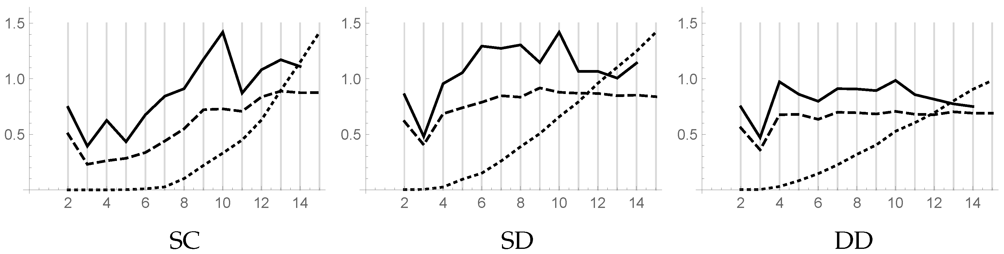
The first experiment concerns the clustering of the three datasets of
Figure 1: dataset
Subcluster (SC) has five clusters, and four of them are subclusters forming two pairs of clusters, respectively; dataset
Skewdistribution (SD) has three clusters with skewed dispersions; dataset
Differentdensity (DD) has clusters with different densities. Each dataset is generated with 1000 points.
We applied
Kvar to each dataset with
k varying in the interval
.
Figure 2 shows the piecewise linear plots versus
k of the DB index (dashed line), DB** index (solid line), and CL index (dotted line) for the three datasets. The CL plot is normalized in order to fit the size of the figure.
For the dataset SC, the DB index suggests choosing , while the DB** index suggests both and , with a weak preference for the former. The plot of the CL index, which is zero for , shows that the clusters in this range of k are well-separated, while for the increase of the plot suggests that some clusters are improperly subdivided.
For both datasets SD and DD, the DB and DB** indexes indicate the same value, 3, for k. The CL plot, which is not zero even for small values of k, reveals the presence of close points in different clusters. The difficulty encountered in the assignment of these points to the clusters suggests that such points could be considered as noise. In any case, using the information gathered from the CL plot, the computation should stop before k becomes too large.
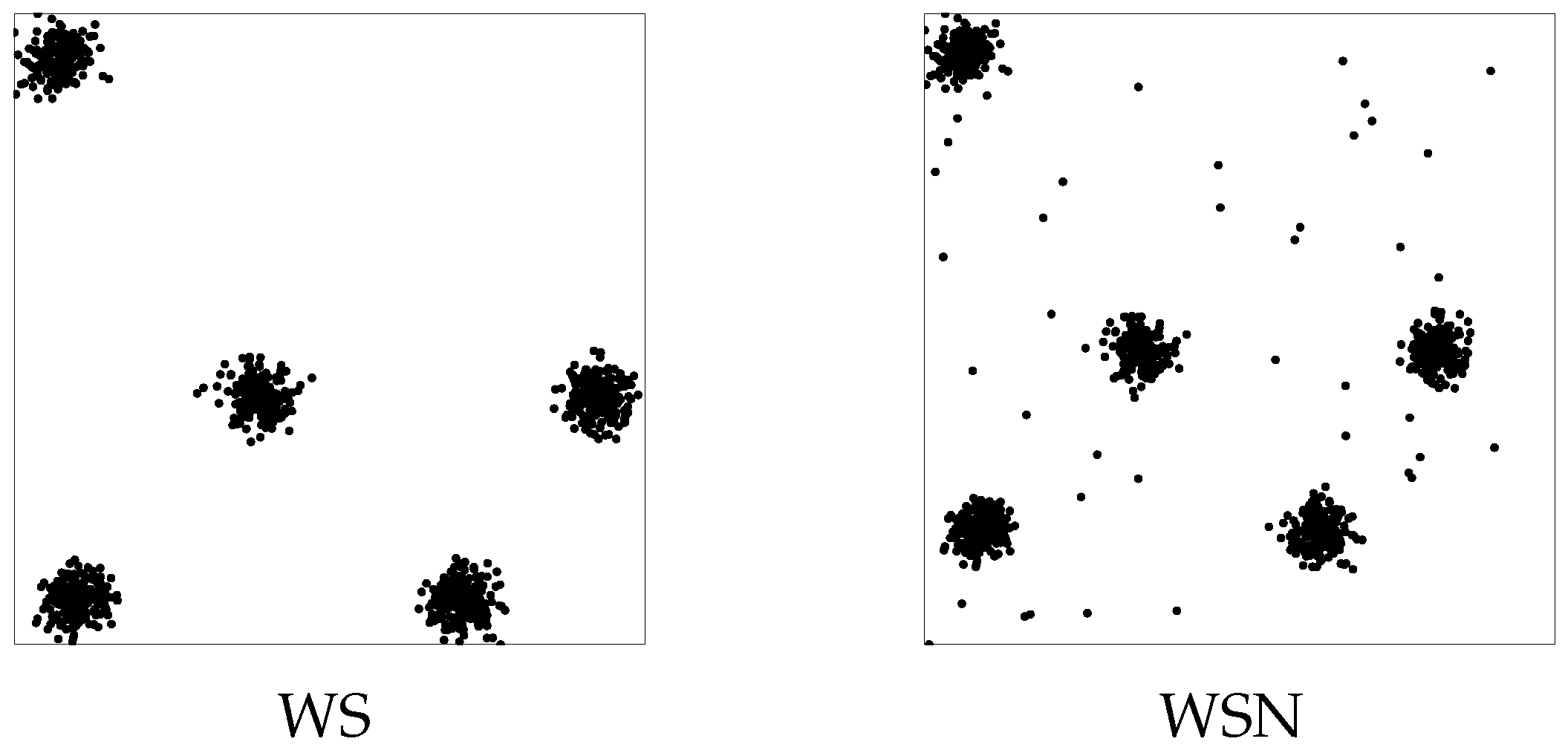
The purpose of the second test is precisely to see how the procedure behaves in the presence of noise. To this aim, the two datasets of five points
Well-separated (WS) and
Well-separated noise (WSN) of
Figure 3 are generated, the latter one with
noise added to the former.
We applied
Kvar, with
k varying in the interval
and obtained the piecewise linear plots versus
k of
Figure 4. For dataset WSN, according to the DB index, both
and
seemed to be acceptable. This uncertainty is explained by the presence of noise which causes spurious clusters to appear. The DB** index correctly suggests
. The presence of noise is confirmed by the CL index which is not zero for small values of
k.
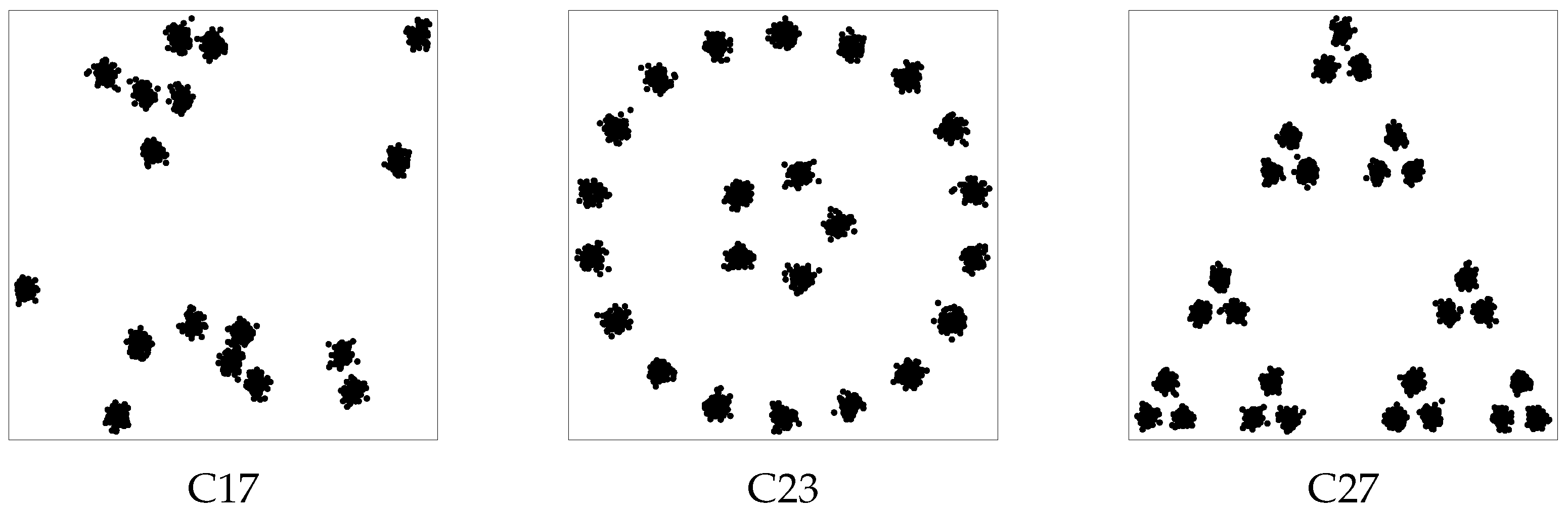
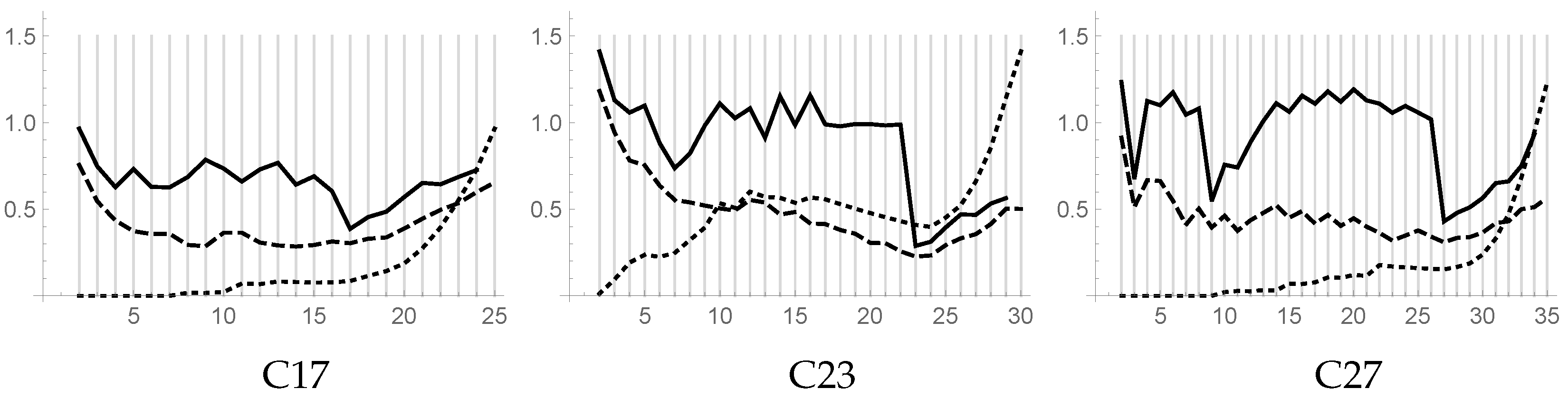
To analyze more thoroughly the performance of our algorithm when subclusters are present, a third experiment was carried out concerning the three datasets of
Figure 5. Dataset C17 consists of 1700 points generated around 17 randomly chosen centers; dataset C23, consisting of 2300 points, has 23 clusters of 100 points which can be grouped in several ways in a lower number of clusters; dataset C27, consisting of 2700 points, has 27 clusters of 100 points which can be seen as 9 clusters of 300 points or three clusters of 900 points, depending on the granularity level of interest.
Problems C17, C23, and C27 have been tested with values of
k ranging in the intervals
,
, and
, respectively. The resulting piecewise linear plots versus
k of DB, DB**, and CL indices are shown in
Figure 6. By using the DB** indices, it clearly appears that our algorithm is able to find good clusterings for all three problems. The inspection of the plot of the DB** index gives further information. For example, for problem C17, a local minimum of the DB** index for
evidences the clustering shown in
Figure 7 on the left. For problem C23, a local minimum of the DB** index for
evidences the possible clustering shown in
Figure 7 on the right. For problem C27, two local minima in the DB** plot for
and
evidence the two other expected clusterings.
In all the experiments shown above, the measure CL helps decide the value of if not assigned.
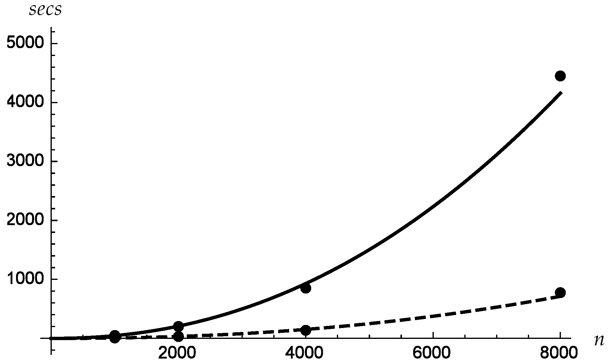
The fourth test regards the computational cost of algorithm
Kvar when run on one or eight processors. Due to its iterative and heuristic structure, our algorithm is not suitable for a theoretical analysis of the complexity. In order to analyze how the required time increases as a function of the number of the points, the datasets SC, SD, DD, WS, and WSN have been generated with
n varying in
and
k varying in the interval
.
Figure 8 shows the plots versus
n of the costs in seconds, averaged on all the datasets. The times corresponding to runs with one processor are fitted with a solid line, where those corresponding to runs with eight processors are fitted with a dashed line. The resulting polynomial fits are
for one processor and
for eight processors. This shows that for the considered problems, the time grows slightly more than quadratically as a function of
n, but clearly less than cubically, as one could expect. It also shows that the whole procedure has a good degree of scalability.
7. Discussion and Conclusions
In this paper, we considered the symmetric modeling of the clustering problem and proposed an algorithm which applies NMF techniques to a penalized nonsymmetric minimization problem. The proposed algorithm makes use of a similarity matrix A, which depends on the Gaussian kernel function and a scale parameter , varying with k. The Gaussian kernel function was chosen because it is widely used in the clustering problems of points in . Of course, other kernels can be used in different environments, with different procedures. We think that our heuristic approach could also be applied to treat other kernels.
As shown in [
1,
13], the ANLS algorithm with the
BPP method handles large datasets more efficiently than other algorithms frequently used for the same problem. Moreover, in [
14], it is shown that ANLS with
GCD allows for further time reduction with respect to ANLS with
BPP.
The proposed heuristic approach, which uses ANLS with GCD, processes multiple instances of the problem and focuses the computation only on the more promising ones, making use of the DB index. In this way, an additional time reduction is achieved with respect to the standard multistart approach. The experimentation, conducted on synthetic problems with different characteristics, evidences the reliability of the algorithm.
The same framework is repeatedly applied with different values of k varying in an assigned interval, allowing us to deal also with the clustering problem when the number of clusters is not a priori fixed. The combined use of the different considered validity indices allows to point out the correct solutions.

