Backstepping Adaptive Neural Network Control for Electric Braking Systems of Aircrafts

Abstract

This paper proposes an adaptive backstepping control algorithm for electric braking systems with electromechanical actuators (EMAs). First, the ideal mathematical model of the EMA is established, and the nonlinear factors are analyzed, such as the deformation of the reduction gear. Subsequently, the actual mathematical model of the EMA is rebuilt by combining the ideal model and the nonlinear factors. To realize high performance braking pressure control, the backstepping control method is adopted to address the mismatched uncertainties in the electric braking system, and a radial basis function (RBF) neural network is established to estimate the nonlinear functions in the control system. The experimental results indicate that the proposed braking pressure control strategy can improve the servo performance of the electric braking system. In addition, the hardware-in-loop (HIL) experimental results show that the proposed EMA controller can satisfy the requirements of the aircraft antilock braking systems.

1. Introduction

With the development of aviation technology, the performance of modern aircraft has also greatly improved and the requirement of braking system performance is more stringent [1,2,3,4,5]. The electric braking system is a new type of braking system that uses electromechanical actuators instead of traditional hydraulic actuators. Compared with the hydraulic braking system, the electric braking system has advantages of light weight, small volume, and high reliability which make it the development direction of aircraft braking systems in the future [6,7,8,9].

As a new type of actuator, the electromechanical actuator (EMA) is composed of a motor, reduction gear, and a ball screw. With the development of permanent magnet material technology, the brushless DC motor (BLDCM) has been widely used in many industrial and automotive applications. The BLDCM has the advantages of a high-power density, a compact structure, and high efficiency which make it suitable for driving the EMA [10,11,12]. From the analysis above, it can be noted that the electric braking system is a new kind of servo system with special applications. Therefore, an appropriate control strategy is needed to satisfy the high-performance requirement of the aircraft braking system.

The EMA is a complex mechatronic transmission system that contains friction, backlash, hysteresis, and other nonlinear factors. These characteristics make it difficult to accurately describe the dynamic mathematical model of the EMA. In addition, aircrafts usually work in harsh environments, such as large fluctuations in temperature, strenuous vibrations, and damp conditions. For these reasons, it is impossible to obtain an accurate mathematical model of the EMA and is therefore difficult for the EMA to achieve the high precision and fast response of the braking pressure control effect with a traditional linear controller. To design an appropriate controller, the mathematical model of the EMA must be reasonably simplified, and many studies have been working on this issue [13,14,15]. The compound disturbance in the EMA is a combination of the internal deformation, external disturbance, time-varying parameters, and unmodeled dynamics, so an appropriate design idea is also essential to design the control law of the electric braking system [16,17].

Peng et al. proposed a sliding mode control method for the electromechanical braking system with a BLDCM, and the switching control law was adjusted by a fuzzy corrector [18]. Li et al. presented a dynamic surface-based control algorithm for solving the stability problem of slip ratio control in an electric braking system [19]. To improve the control ability and accuracy of the motor in a flexible-joint robot, a fuzzy PID control method was proposed in [20]. To overcome the parameter variability and unknown disturbance in the electric rudder servo system, Lv et al. proposed a backstepping power fast terminal sliding mode control algorithm in [21]. Liang et al. [22] designed an RBF neural network-based nonsingular fast terminal sliding mode control algorithm for braking systems with an EMA. The global stability of the control law was proved by using the Lyapunov function. In [23], Chen et al. proposed a sliding-mode extremum seeking controller for the all-electric active braking system in unmanned aerial vehicles and validated the servo performance of the designed controller through HIL experiments. Lin et al. [24] realized a non-mechanical antilock braking system (ABS) controller for the electric scooter, and the braking performance for the ABS action was further addressed via experiments.

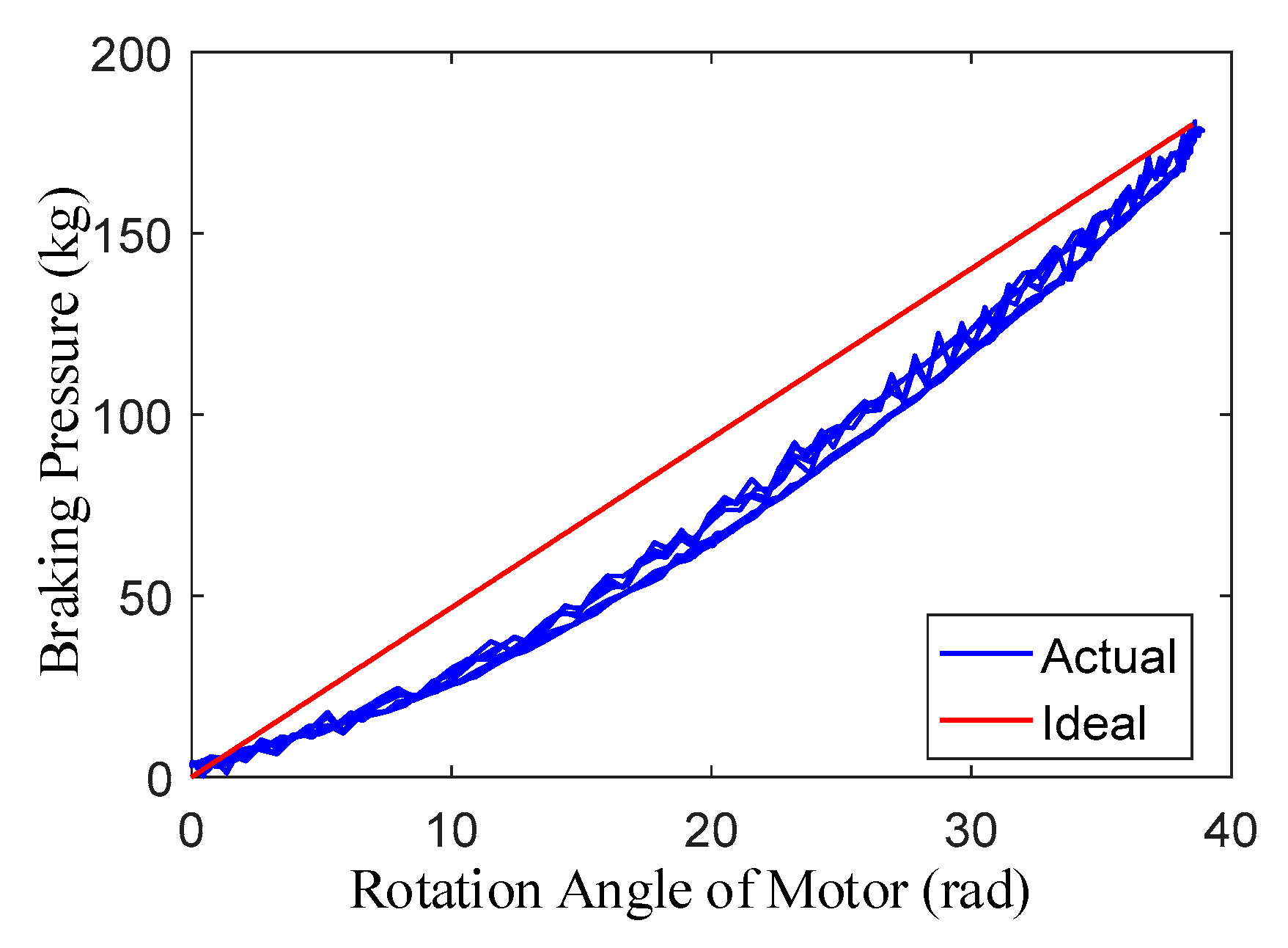
Furthermore, most of the existing studies have focused on improving the performance of the EMA controller, and the braking pressure-motor angle models in the literature are generally equivalent to a first-order proportional linear model. However, as shown in Figure 2, the real curve of the EMA is not the case. Therefore, the traditional first-order mathematical model is not accurate enough to describe the actual EMA model. On the basis of [22], the deformation of the reduction gear under braking pressure is analyzed and combined with the ideal EMA mathematical model, and subsequently, the actual EMA mathematical model is rebuilt. The backstepping control method has shown its effectiveness in dealing with systems with multiple dynamics and mismatched uncertainties, but a major problem is that certain functions must be linear in the unknown parameters and tedious analysis is needed to determine the regression matrices. The RBF neural network has strong input and output mapping functions, which make it suitable to use a stable neural network controller to estimate certain nonlinear functions. With the help of RBF neural networks, the linear-in-the-parameters assumption of the nonlinear function and the determination of the regression matrices can be avoided. According to the characteristics of the actual EMA model, an adaptive backstepping control method is proposed and the RBF neural network is used to address the uncertain compound disturbance of the electric braking system. Compared with the routine control strategies, the servo performance of the braking pressure and the adaptive ability of the control system are improved significantly.

The remainder of this paper is organized as follows: Section 1 introduces the control problems of the electric braking system in aircrafts. Section 2 presents the working principle of the electric braking system and structure of the EMA. Then, the deformation of the reduction gear is analyzed in detail, the actual EMA mathematical model is established, and the corresponding control target is put forward. Section 3 presents the backstepping adaptive controller and the design method of the RBF neural network, and the stability analysis of the proposed controller is carried out using Lyapunov functions. Section 4 discusses the experimental results and the hardware in loop experiments. The conclusions are summarized in Section 5.

The main contributions of this paper are summarized as follows: first, the paper analyzed the ideal EMA mathematical model and the nonlinear factors, and then the actual EMA mathematical model is rebuilt by considering the deformation of the reduction gear. Second, the proposed adaptive nonlinear control method can overcome the nonlinear factors of the electric braking system and improve the response speed and control precision of the EMA. Third, the control effect of the newly designed EMA controller is fully validated through the HIL experiments.

2. Mathematical Model of the EMA

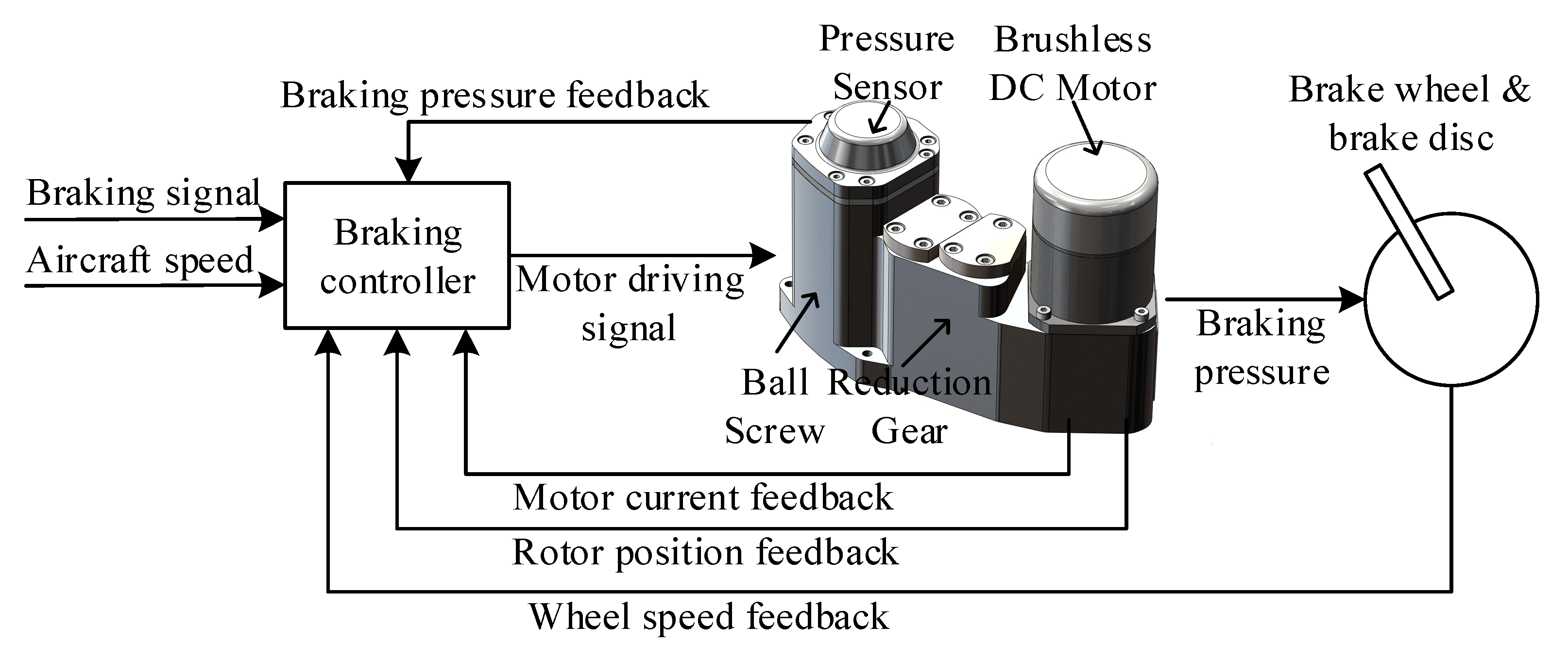
The electric braking system is composed of a braking controller, an EMA, a brake wheel, and a brake disc. The structure of the electric braking system in the aircraft is shown in Figure 1. The braking controller is the control and drive unit of the braking system. Its functions include braking signal receiving, data processing, and control algorithm implementation. Then, the corresponding motor driving signal is generated and used to drive the EMA to realize the braking actions. The braking pressure feedback, motor current feedback, and the rotor position feedback signals are also transformed to the braking controller, which will be used to achieve the braking pressure closed-loop control.

At the same time, the aircraft speed and wheel speed are used to calculate the slip ratio, which is usually used in the antilock braking system to prevent wheels from locking. The slip ratio control is also finished in the braking controller by controlling the output braking pressure signal. No more expatiation is needed here as there are many studies.

2.1. Ideal EMA Mathematical Model

The brushless DC motor (BLDCM) is usually controlled through a variable armature voltage. To simplify the mathematical model of the EMA, the following assumptions are made: the current fluctuation caused by the commutations is ignored, the magnetic condition of the motor is unsaturated, and the hysteresis losses and the eddy-current losses are ignored.

The voltage equation and torque equation of the BLDCM are expressed as:

$$\{\begin{array}{l}L\dot{i}=-Ri-E_a+U_a\\ J{\dot{\omega }}_m=-B_v{\omega }_m+T_e-T_L\\ T_e=k_{T}i,E_a=k_{emf}{\omega }_m\end{array},$$

(1)

where $U_a$ is the armature voltage, $R$ is the stator resistance, $i$ is the armature current, $L$ is the stator inductance, $E_a$ is the back electromotive force, $k_{emf}$ is the back electromotive force constant, $J$ is the inertia moment, ${\omega }_m$ is the mechanical speed of the motor, $B_v$ is the viscous damping coefficient, $T_e$ is the electromagnetic torque, $k_T$ is the torque constant, and $T_L$ is the load torque.

The relationship between the vertical motion of the ball screw and the rotary motion of the motor is shown as:

$${\dot{x}}_{ema}=L_0{\omega }_m/2\pi \eta ,$$

(2)

where $x_{ema}$ is the axis displacement of the EMA, $L_0$ is the lead of the ball screw, and $\eta$ is the transmission ratio of the reduction gear.

By considering the essential characteristic of the electric braking system, the output braking pressure of the EMA can be calculated as:

$$p=c_b(x_{ema}-x_b),$$

(3)

where $p$ is the braking pressure of the EMA, $c_b$ is the stiffness coefficient of the brake disc and $x_b$ is the lateral displacement of the brake disc.

If the lateral displacement of the brake disc is assumed to be zero, Equation (3) can be simplified as:

$$p=c_b{x}_{ema}.$$

(4)

The load torque of the motor ($T_L$) can be divided into two parts: part of it is used to overcome the resistance torque of the ball screw, and the remainder is used to overcome the drive torque of the ball screw. Then, the load torque can be calculated using the following equation:

$$T_L=T_{rt}+T_{dt},$$

(5)

where $T_{rt}$ is the resistance torque of the ball screw and $T_{dt}$ is the drive torque of the ball screw.

In the EMA of the electric braking system, the resistance torque $T_{rt}$ is assumed to be a constant value, and the drive torque $T_{dt}$ is related to the output braking pressure $p$. In most studies, $T_{dt}$ is equivalent to a linear function of the braking pressure as:

$$T_{dt}=p{L}_0/2\pi \eta .$$

(6)

However, this simplification has a significant effect on the control performance of the electric braking system. By analyzing the electric braking system, it can be found that when the changing rate of the braking pressure $\dot{p}$ is positive, the drive torque is a resistance to the motor. When the changing rate of the braking pressure $\dot{p}$ is negative, the drive torque is a motivation to the motor, as shown in Equation (7):

$$T_{dt}=p\mathrm{sgn}(\dot{p})L_0/2\pi \eta$$

(7)

To decrease the chattering of the braking pressure control effect, a saturation function is introduced instead of the sign function. According to Equations (2) and (4), the load of the motor can be expressed as:

$$T_L=T_{rt}+p\mathrm{sat}({\omega }_m,\tau )L_0/2\pi \eta ,$$

(8)

where the saturation function is defined as:

$$\mathrm{sat}({\omega }_m,\tau )=\{\begin{array}{ll}1,& {\omega }_m>\tau \\ {\omega }_m/\tau ,& \left|{\omega }_m\right|\le \tau \\ -1,& {\omega }_m<-\tau \end{array},$$

(9)

where $\tau$ is the boundary coefficient of the saturation function.

By taking consideration of Equations (1)—(9), selecting the state variables as $x_i=\left[p,{\omega }_m,i\right]$, the ideal mathematical model of the EMA can be expressed as:

$$\{\begin{array}{l}\dot{p}=c_b{L}_0{\omega }_m/2\pi \eta \\ {\dot{\omega }}_m=J^{-1}(-B_v{\omega }_m+k_{T}i-T_L)\\ \dot{i}=L^{-1}(-Ri-k_{emf}{\omega }_m+U_a)\end{array}$$

(10)

$$T_L=T_{rt}+p\mathrm{sat}({\omega }_m,\tau )L_0/2\pi \eta$$

(11)

2.2. Deformation of the Reduction Gear

As seen from Equation (10), the relationship between the braking pressure $p$ and the rotation angle of motor ${\theta }_m$ is established by a linear function. However, the ideal EMA mathematical model ignored many nonlinear factors, such as the deformation of the gear and gear clearance. As described in the literature [25,26], the reduction gear will exhibit deformation under a heavy load which can eventually affect the relationship between the braking pressure and the motor position, rendering it different from the ideal model. After many experiments, the actual curves of the braking pressure and the motor position are drawn and the comparison of the ideal and actual curves is shown in Figure 2.

It was assumed that the deformation of the reduction gear under the braking pressure $p$ is ${\delta }_g$, and ${\delta }_g$ is divided into two parts: the contact deformation ${\delta }_{g1}$ and the bending deformation ${\delta }_{g2}$.

When analyzing the contact deformation of the reduction gear ${\delta }_{g1}$, it can be simplified as a contact force model of two cylinders with parallel axes. If the contact force is small, then the two cylinders can be thought of as touching along a line parallel to their axes. As the contact force increases, the contact line deforms into a contact surface along with the elastic deformation of the material. The interface width $w_g$ can be determined by the gear parameters, and the interface length $l_g$ can be determined from the Hertz theory [27]:

$$l_g=1.596\sqrt{f_g\cos {\alpha }_g{\rho }_g(1-{\mu }_g^2)/E_g},$$

(12)

where ${\alpha }_g$ is the angle between the acting force $f_g$ and the $y$ axis,${\rho }_g$ is the radius of curvature of the contact surface,${\mu }_g$ and $E_g$ are the elastic constants of the reduction gear.

Then, the stress in the reduction gear can be expressed as:

$${\sigma }_g=\frac{f_g}{l_g{w}_g}.$$

(13)

The contact deformation of the reduction gear can be calculated using Hooke’s law:

$${\delta }_{g1}=\frac{f_g{p}_g}{l_g{w}_g{E}_g}$$

(14)

For a fixed reduction gear, all of the parameters are constants except for the acting force $f_g$. Then, Equation (14) can be simplified as:

$${\delta }_{g1}=c_{g1}\sqrt{f_g},$$

(15)

where $c_{g1}$ is a constant, which is determined by the reduction gear parameters.

When analyzing the bending deformation of the reduction gear ${\delta }_{g2}$, the research should focus on the deformation of the meshing point so the distributed force along the tooth surface is simplified into a concentrated force, and the reduction gear is regarded as a cantilever of the elastic material. The force component in the $y$ axis of the acting force $f_g$ is represented as $f_{gy}$:

$$f_{gy}=f_g\cos {\alpha }_g.$$

(16)

The bending deformation of the reduction gear under $f_{gy}$ in the $y$ axis is expressed as:

$${\delta }_{gy}=\frac{r_g{f}_g{\cos }^2{\alpha }_g}{E_g{I}_g}{\displaystyle \underset{0}{\overset{t}{\int }}\Delta x_g^{2}t\cos tdt},$$

(17)

where $r_g$ is the radius of the gear base,${\alpha }_g$ is the angle between $f_g$ and the $y$ axis, $E_g$ is the elasticity modulus of the gear, $I_g$ is the section modulus of the gear and $\Delta x_g$ is the arm length of the equivalent bending moment.

Then, the bending deformation of the gear is generated as:

$${\delta }_{g2}={\delta }_{gy}\cos {\alpha }_g.$$

(18)

Similarly, all of the parameters are constants except for the acting force $f_g$. Equations (17) and (18) can be simplified as:

$${\delta }_{g2}=c_{g2}{f}_g,$$

(19)

where $c_{g2}$ is a constant, which is determined by the reduction gear parameters.

After the deformation analysis, the relationship between the braking pressure $p$ and the acting force $f_g$ is needed. It is expressed as:

$$f_g=p{l}_0/2\pi \eta$$

(20)

Then, the deformation of the reduction gear under the braking pressure is generated as:

$$\{\begin{array}{l}{\delta }_{g1}=c_{g1}\sqrt{p{l}_0/2\pi \eta }\\ {\delta }_{g2}=c_{g2}p{l}_0/2\pi \eta \end{array}$$

(21)

2.3. Actual EMA Mathematical Model and the Control Target

If there is no deformation in the reduction gear, then it can be generated from Equations (2) and (4) that the ideal relationship between the braking pressure $p$ and the motor position $\Delta {\theta }_m$ is:

$$p=c_b{L}_0\Delta {\theta }_m/2\pi \eta .$$

(22)

Considering the deformation in the reduction gear by combining Equations (21) and (22), the relationship between the braking pressure and the motor angle can be expressed by a second order equation [28,29,30]. Then, it can be obtained by using on a least square fit in Figure 2 as:

$$p=c_1\Delta {\theta }_m+c_2{\left(\Delta {\theta }_m\right)}^2,$$

(23)

where $c_1$ and $c_2$ are constants, and they are determined by the EMA parameters.

Finally, in the EMA mathematical model, the quadratic item in Equation (23) is treated as a disturbance item. By taking the state variables $x_i=\left[p,{\omega }_m,i\right]$ into the equations, the actual state space model of the EMA is expressed as:

$$\{\begin{array}{l}{\dot{x}}_1=a_1{x}_2+f_1(\mathbf{x})\\ {\dot{x}}_2=a_2{x}_3+f_2(\mathbf{x})\\ {\dot{x}}_3=a_3{U}_a+f_3(\mathbf{x})\\ y=x_1\end{array},$$

(24)

where $a_1=c_b{L}_0/2\pi \eta$, $a_2=J^{-1}{k}_T$, $a_3=L^{-1}$. $f_1(\mathbf{x})$, $f_2(\mathbf{x})$ and $f_3(\mathbf{x})$ are unknown continuous functions of the variables $x_i=\left[p,{\omega }_m,i\right]$.

The corresponding control target is proposed as follows: design a braking pressure controller of the EMA mathematical model described in Equation (24) so that the braking pressure $p$ can track the desired braking pressure $p^{\ast }$ without errors in finite time.

It can be found that the electric braking system is essentially a high-performance pressure servo system which is driven by a BLDCM, and the controller design needs to consider the model uncertainty and the disturbance from the system. The unknown function comes from the deformation of the EMA and the nonlinear load torque of the motor, where the disturbance is mainly caused by parameter perturbation and the unmodeled dynamics of frictions. Therefore, the control algorithm to be designed needs to overcome these unknown disturbances to achieve high performance pressure control.

3. Control Strategy

The backstepping control method can decompose the complex nonlinear system into several sub systems, and the corresponding Lyapunov function of the whole system can be derived step by step [31,32]. According to the characteristics of the actual EMA mathematical model, this paper proposes an adaptive backstepping control method that uses an RBF neural network to approximate and adaptively cancel the unknown parts of the system.

To facilitate the design of the controller, the assumption that the reference braking pressure signal $p^{\ast }$ is continuous and its derivative exists is made.

3.1. Controller Design

Based on the backstepping theory, the high order system is divided into three sub systems, and the Lyapunov function of the system is built [33,34]. The error variables of system are defined as:

$$\{\begin{array}{l}{e}_1=x_1-p^{*}\\ e_2=x_2-{\alpha }_1\\ e_3=x_3-{\alpha }_2\end{array},$$

(25)

where $e_1$, $e_2$, $e_3$ are the errors,${\alpha }_1$ and ${\alpha }_2$ are the virtual control variables of the sub system.

Step 1:

For the first sub system, the Lyapunov function is selected as:

$$V_1=\frac{e_1^2}{2}.$$

(26)

Obtain the derivative of Equation (26) as:

$${\dot{V}}_1=e_1{\dot{e}}_1=e_1\left(a_1{e}_2+a_1{\alpha }_1+f_1(\mathbf{x})-{\dot{p}}^{\ast }\right).$$

(27)

The virtual control variable ${\alpha }_1$ is designed as:

$${\alpha }_1=\frac{1}{a_1}\left(-{\mu }_1{e}_1-{\widehat{f}}_1(\mathbf{x})+{\dot{p}}^{\ast }\right).$$

(28)

Take Equation (28) into Equation (27) as:

$${\dot{V}}_1=a_1{e}_1{e}_2+e_1{\Delta }_1(\mathbf{x})-{\mu }_1{e}_1^2,$$

(29)

where ${\widehat{f}}_1(\mathbf{x})$ is the designed neural network function, which will be used to approximate the unknown continuous function $f_1(\mathbf{x})$, and ${\Delta }_1(\mathbf{x})=f_1(\mathbf{x})-{\widehat{f}}_1(\mathbf{x})$ is the estimated error.

Step 2:

For the second sub system, the item $e_1{e}_2$ in (29) needs to be offset, and the Lyapunov function is selected as:

$$V_2=V_1+\frac{e_2^2}{2}.$$

(30)

Obtain the derivative of Equation (30) as:

$${\dot{V}}_2={\dot{V}}_1+e_2{\dot{e}}_2={\dot{V}}_1+e_2\left(a_2{e}_3+a_2{\alpha }_2+f_2(\mathbf{x})-{\dot{\alpha }}_1\right).$$

(31)

The virtual control variable ${\alpha }_2$ is designed as:

$${\alpha }_2=\frac{1}{a_2}\left(-a_1{e}_1-{\mu }_2{e}_2-{\widehat{f}}_2(\mathbf{x})+{\dot{\alpha }}_1\right).$$

(32)

Take Equation (32) into Equation (31) as:

$${\dot{V}}_2={\displaystyle \sum _{i=1}^2\left(-{\mu }_i{e}_i^2+e_i{\Delta }_i(\mathbf{x})\right)}+a_2{e}_2{e}_3,$$

(33)

where ${\widehat{f}}_2(\mathbf{x})$ is the designed neural network function, which will be used to approximate the unknown continuous function $f_2(\mathbf{x})$, and ${\Delta }_2(\mathbf{x})=f_2(\mathbf{x})-{\widehat{f}}_2(\mathbf{x})$ is the estimated error.

Step 3:

For the third sub system, the Lyapunov function is selected as:

$$V_3=V_2+\frac{e_3^2}{2}.$$

(34)

Obtain the derivative of Equation (34) as:

$${\dot{V}}_3={\dot{V}}_2+e_3{\dot{e}}_3={\dot{V}}_2+e_3\left(a_3{U}_a+f_3(\mathbf{x})-{\dot{\alpha }}_2\right).$$

(35)

The control law of $U_a$ is designed as:

$$U_a=\frac{1}{a_3}\left(-a_2{e}_2-{\mu }_3{e}_3-{\widehat{f}}_3(\mathbf{x})+{\dot{\alpha }}_2\right).$$

(36)

Take Equation (36) into Equation (35) as:

$${\dot{V}}_3={\displaystyle \sum _{i=1}^3\left(-{\mu }_i{e}_i^2+\frac{e_i}{a_i}{\Delta }_i(\mathbf{x})\right)},$$

(37)

where ${\widehat{f}}_3(\mathbf{x})$ is the designed neural network function, which will be used to approximate the unknown continuous function $f_3(\mathbf{x})$, and ${\Delta }_3(\mathbf{x})=f_3(\mathbf{x})-{\widehat{f}}_3(\mathbf{x})$ is the estimated error.

After the control variable $U_a$ is designed, we need to design the neural network function ${\widehat{f}}_i(\mathbf{x})$ $i=1,2,3$ and keep the control system stable.

3.2. The RBF Neural Network

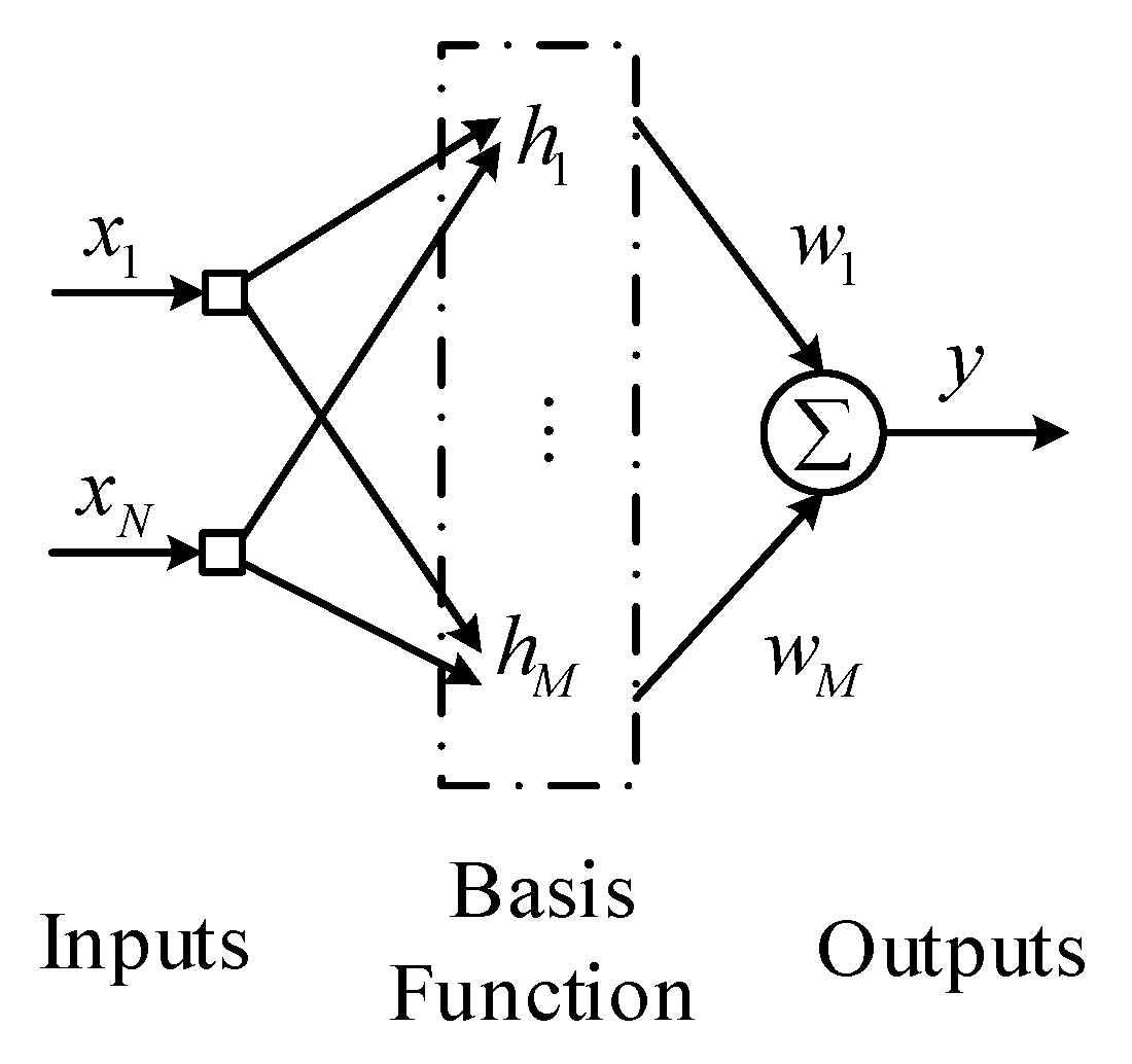
The structure of an RBF neural network is shown in Figure 3.

In Figure 3, the RBF neural network consists of the input layer, the basis function layer (hidden layer), and the output layer [35,36]. The input layer is used to complete the information transfer, the basis function layer is the respective field, and the output layer is the outputs of the RBF neural network. The numbers of the input layer and the output layer are usually determined by the characteristics of the control system. In this paper, there are three neurons in the input layer and one neuron in the output layer. A k-means clustering algorithm is used on selecting the number of the hidden layer and the corresponding control parameters of the neural network [37], and the number of neurons in the hidden layer is eventually determined to be five.

The Gaussian function is chosen as the radial basis function, as shown in Equation (38):

$$h_i(x)=\exp \left(-\frac{{\Vert x-c_i\Vert }^2}{2d_i^2}\right)i=1,2,\cdots M,$$

(38)

where $c_i$ is the center of the basis function,$d_i$ is the scaling factor of the basis function, and $h_i(·)$ is the base Gaussian function.

From Equation (37), it can be found that there are three unknown functions $f_1$, $f_2$ and $f_3$, so we use three RBFs to approximate them as follows (39):

$$\{\begin{array}{l}{f}_1=W_1^T{H}_1+{\epsilon }_1\\ f_2=W_2^T{H}_2+{\epsilon }_2\\ f_3=W_3^T{H}_3+{\epsilon }_3\end{array},$$

(39)

where $W_i$ is the ideal neural network weight vector and $W_i={\left[w_{1i} w_{2i} w_{3i} w_{4i} w_{5i}\right]}^T$, $w_{Mi}(M=1,2,3,4,5)$ is the weight value, $H_i$ is the radial basis vector, and $H_i={\left[h_{1i} h_{2i} h_{3i} h_{4i} h_{5i}\right]}^T$, $h_{Mi}(M=1,2,3,4,5)$ is the Gaussian function, ${\epsilon }_i$ is the approximation error,$i=1,2,3$, and $\Vert \epsilon \Vert =\Vert {\left[{\epsilon }_1{\epsilon }_2{\epsilon }_3\right]}^T\Vert \le {\epsilon }_N$, ${\Vert W_i\Vert }_F\le W_M$ ($\Vert \epsilon \Vert$ is the Euclidean norm of $\epsilon$, ${\Vert W_i\Vert }_F$ is the Forbenius norm of $W_i$).

Define ${\widehat{f}}_1$, ${\widehat{f}}_2$ and ${\widehat{f}}_3$ as follows (40):

$$\{\begin{array}{l}{\widehat{f}}_1={\widehat{W}}_1^T{H}_1\\ {\widehat{f}}_2={\widehat{W}}_2^T{H}_2\\ {\widehat{f}}_3={\widehat{W}}_3^T{H}_3\end{array},$$

(40)

where ${\widehat{W}}_i$ is the weight vector estimation.

Similarly, define $Z$, $\widehat{Z}$ and $\tilde{Z}$ as follows (41):

$$Z=\left[\begin{array}{lll}{W}_1& & \\ & W_2& \\ & & W_3\end{array}\right],{\Vert Z\Vert }_F\le {{\rm Z}}_M,\widehat{Z}=\left[\begin{array}{lll}{\widehat{W}}_1& & \\ & {\widehat{W}}_2& \\ & & {\widehat{W}}_3\end{array}\right],\tilde{Z}=Z-\widehat{Z}.$$

(41)

Design the Lyapunov function as:

$$V=\frac{1}{2}{\xi }^T\xi +\frac{1}{2}\mathrm{tr}\left({\tilde{Z}}^T{\mathsf{\Gamma }}^{-1}\tilde{Z}\right),$$

(42)

where $V_3=\frac{1}{2}{\xi }^T\xi$, ${\Vert Z\Vert }_F$ is the Forbenius norm of $Z$, $\mathsf{\Gamma }$ is a positive definite matrix with proper dimensions, $\mathsf{\Gamma }=\left[\begin{array}{lll}{\mathsf{\Gamma }}_1& & \\ & {\mathsf{\Gamma }}_2& \\ & & {\mathsf{\Gamma }}_3\end{array}\right]$, $\xi ={\left[e_1{e}_2{e}_3\right]}^T$.

Design the RBF neural network weights adaptive law as follows:

$$\dot{\widehat{Z}}=\mathsf{\Gamma }H{\xi }^T-n\mathsf{\Gamma }\Vert \xi \Vert \widehat{Z},$$

(43)

where $H={\left[H_1{H}_2{H}_3\right]}^T$, $\Vert \xi \Vert$ is the Euclidean norm of $\xi$, and $n>0$.

From Equation (42), we have

$$\dot{V}={\xi }^T\dot{\xi }+\mathrm{tr}\left({\tilde{Z}}^T{\mathsf{\Gamma }}^{-1}\dot{\tilde{Z}}\right)={\displaystyle \sum _{i=1}^3\left(-{\mu }_i{e}_i^2\right)}+{\displaystyle \sum _{i=1}^3\left({\tilde{W}}_i^T{H}_i+{\epsilon }_i\right)e_i}+\mathrm{tr}\left({\tilde{Z}}^T{\mathsf{\Gamma }}^{-1}\dot{\tilde{Z}}\right),$$

(44)

where ${\tilde{W}}_i^T=W_i^T-{\widehat{W}}_i^T$ and $i=1,2,3$.

Then we can obtain:

$$\dot{V}=-{\xi }^{T}K\xi +{\xi }^{T}E+{\xi }^T\tilde{Z}H+\mathrm{tr}\left({\tilde{Z}}^T{\mathsf{\Gamma }}^{-1}\dot{\tilde{Z}}\right)=-{\xi }^{T}K\xi +{\xi }^{T}E+\mathrm{tr}\left({\tilde{Z}}^T{\mathsf{\Gamma }}^{-1}\dot{\tilde{Z}}+{\tilde{Z}}^{T}H{\xi }^T\right),$$

(45)

where $K={\left[{\mu }_1{\mu }_2{\mu }_3\right]}^T$, and $E={\left[{\epsilon }_1{\epsilon }_2{\epsilon }_3\right]}^T$.

Since $\dot{\tilde{Z}}=-\dot{\widehat{Z}}$, by using the RBF network weights adaptive law in (43), $\dot{V}$ is expressed as:

$$\dot{V}=-{\xi }^{T}K\xi +{\xi }^{T}E+n\Vert \xi \Vert \mathrm{tr}\left({\tilde{Z}}^T\left(Z-\tilde{Z}\right)\right).$$

(46)

If $K_{\min }$ is the minimum eigenvalue of $K$, then we can know that $K_{\min }{\Vert \xi \Vert }^2\le {\xi }^{T}K\xi$, according to the Schwarz inequality, it can be found that

$$\mathrm{tr}\left({\tilde{Z}}^T\left(Z-\tilde{Z}\right)\right)\le {\Vert \tilde{Z}\Vert }_F{\Vert Z\Vert }_F-{\Vert \tilde{Z}\Vert }_F^2.$$

(47)

Take (47) into (46), we can obtain:

$$\begin{array}{ll}\dot{V}& \le -K_{\min }{\Vert \xi \Vert }^2+{\epsilon }_N\Vert \xi \Vert +n\Vert \xi \Vert \left({\Vert \tilde{Z}\Vert }_F{\Vert Z\Vert }_F-{\Vert \tilde{Z}\Vert }_F^2\right)\\ & \le -\Vert \xi \Vert \left(K_{\min }\Vert \xi \Vert -{\epsilon }_N+n{\Vert \tilde{Z}\Vert }_F\left({\Vert \tilde{Z}\Vert }_F-Z_M\right)\right)\end{array}.$$

(48)

Since $K_{\min }\Vert \xi \Vert -{\epsilon }_N+n{\Vert \tilde{Z}\Vert }_F\left({\Vert \tilde{Z}\Vert }_F-Z_M\right)=K_{\min }\Vert \xi \Vert -{\epsilon }_N+n{\left({\Vert \tilde{Z}\Vert }_F-\frac{1}{2}{Z}_M\right)}^2-\frac{n}{4}{Z}_M^2$, if we can ensure that $\Vert \xi \Vert >\frac{4{\epsilon }_N+n{Z}_M^2}{4K_{\min }}$, then $\dot{V}\le 0$ will be true, and the control system will be stable. By adjusting the parameters ${\epsilon }_N$, $n$ and $K_{\min }$ properly, the dynamic performance of the controller will be improved.

Compared to the traditional backstepping control method, the RBF backstepping control method in this paper has strong robustness, benefiting from the universal approximation character of the RBF neural network.

4. Results and Analysis

To verify the servo performance of the proposed control method, the signal generator is taken as the braking pressure reference signal source, and a scope is used to record the braking pressure signals. For practical purposes, the EMA is installed in the aircraft wheel as shown in Figure 4a, and the HIL test bench is shown in Figure 4b.

First, we need to design the control parameters of the neural networks, including the cluster centers of the basis function, the scaling factors of the basis function, and the weight value vectors of the output layer. As mentioned above, a k-means clustering algorithm is adopted to calculate the cluster centers and the scaling factors, and the weight value vectors can be obtained by a pseudo-inverse method. The workflow of the k-means is shown as follows:

(1) Selecting $M$ different vectors as the initial cluster center $c_1(0),c_2(0),\dots ,c_M(0)$, where $M$ is the number of the hidden nodes.

(2) Calculating the Euclidean distance between each input sample point and the clustering center point, as shown Equation (49), and $X^p$ is the sample data.

$$\Vert X^p-c_j(k)\Vert ,p=1,2,\dots ,P;j=1,2,\dots ,M.$$

(49)

(3) Classifying the similar sample points into a class. When Equation (50) is satisfied, $X^p$ is classified as the $j^{*}$ class. Then, all of the samples are divided into $M$ subsets as $U_1(k),U_2(k),\dots ,U_M(k)$, and each of them is a clustering domain, which can be represented by the corresponding cluster center.

$$j^{*}(X^p)=\underset{j}{\min }\Vert X^p-c_j(k)\Vert ,p=1,2,\dots ,P.$$

(50)

(4) Modifying the cluster centers by calculating the average values of the samples in each subset. It is calculated as Equation (51):

$$c_j(k+1)=\frac{1}{N_i}{\displaystyle \sum _{X\in U_j(k)}X}{U}_j(k),$$

(51)

where $U_j(k)$ is the j-th cluster domain, and $N_i$ is the samples number of $U_j(k)$.

(5) Let k = k + 1, and turns to step (2). Then repeat the process until the change in $c_j(k)$ is less than the preset threshold.

After the cluster centers are determined, the scaling factors can be obtained as:

$$d_j=\gamma \min \Vert c_j-c_i\Vert .$$

(52)

4.1. RBF Neural Networks Appropximate Performance

Then, the approximate performance of the designed RBF neural networks is verified by real-time experiments. As the neural networks proposed in this paper is used to approximate the unknown functions in the EMA model, we took a set of actual braking pressure data to verify it. The braking pressure ranges from 20 kg to 190 kg, the actual braking pressure and the ideal braking pressure are as shown in Figure 5a. It can be found that there are some differences between the actual pressure and the ideal model, due to the nonlinear factors such as the gear deformation. So, the proposed neural networks are used to approximate the unknown functions in the EMA model and its approximate performance of the braking pressure error is shown in Figure 5b. The experiments results indicate that the neural networks can approximate the braking pressure error effectively. This is also the basis of the high-performance pressure control.

4.2. EMA Servo Performance

Subsequently, the servo performance of the EMA is verified by experiments. The sine wave and square wave are taken as the pressure reference signals respectively, and the reference signal and actual pressure signal are both recorded by the scope. To provide a sufficient comparison, a traditional proportional integral derivative (PID) controller is designed according to the requirements of the electric braking system, and the transfer function is:

$$C(s)=K_p+K_i/s+K_{d}s.$$

(53)

Due to the particularity of the electric braking system, the parameters of the PID controller is designed in two stages: when the braking pressure is increasing, the parameters is $K_p=18$, $K_i=0.02$, $K_d=0.5$, and when the braking pressure is decreasing, the parameters is $K_p=12$, $K_i=0.13$, $K_d=0.2$.

In the proposed braking controller, three RBFs are designed. For each Gaussian function, the parameters of $c_i$ and $d_i$ are designed as [−8, 3, 0, 3, 8] and 20. The initial weight value of each neural net in the hidden layer is selected as 0.90. The parameters in the adaptive law is designed as ${\mu }_1={\mu }_2={\mu }_3=8$, ${\mathsf{\Gamma }}_1=\mathrm{diag}\left\{80,80,80\right\}$, ${\mathsf{\Gamma }}_2=\mathrm{diag}\left\{15,15,15\right\}$, ${\mathsf{\Gamma }}_3=\mathrm{diag}\left\{0.9,0.9,0.9\right\}$, and $n=0.2$.

Figure 6a,b shows that the frequency of the pressure signal is 3 Hz, the amplitude is 300 kg and the offset is 30 kg. It can be found that the proposed control algorithm in this paper has better tracking accuracy and smaller signal phase lag than the PID control algorithm. In Figure 6c,d, the reference signal is a square wave, which requires a more precise control algorithm. The frequency is 2 Hz, the amplitude is 300 kg, and the offset is 30 kg. Compared with the traditional PID control, the proposed method can increase the braking pressure much more quickly without overshot and the static error is much smaller than that in the PID control.

4.3. HIL Experimental Results

In practical work, the braking pressure signal is more irregular which requires higher control performance of the EMA. To verify the control effects of the proposed EMA controller in an actual working environment of the aircraft, an aircraft electric braking system HIL test bench was built as shown in Figure 4b. The aircraft landing model and the antilock controller were established by MATLAB-Simulink and downloaded to the target board. Then, the reference pressure signal was output to the EMA controller and the corresponding braking pressure is realized by EMA. The main structure of the HIL test bench was analyzed in research [14] and no more detail is provided here. The control target of the HIL experiment is to control the slip ratio around the optimal value to maintain the maximum adhesive coefficient between the aircraft wheel and the runway. The slip ratio $\lambda$ and adhesive coefficient $\mu$ are defined as:

$$\lambda =\left(V_x-V_w\right)/V_x,$$

(54)

$$\mu (\lambda )=c_1(1-e^{-c_2\lambda })-c_3\lambda ,$$

(55)

where $V_x$ is the aircraft speed,$V_w$ is the wheel speed, and $c_1$, $c_2$, $c_3$ are constants.

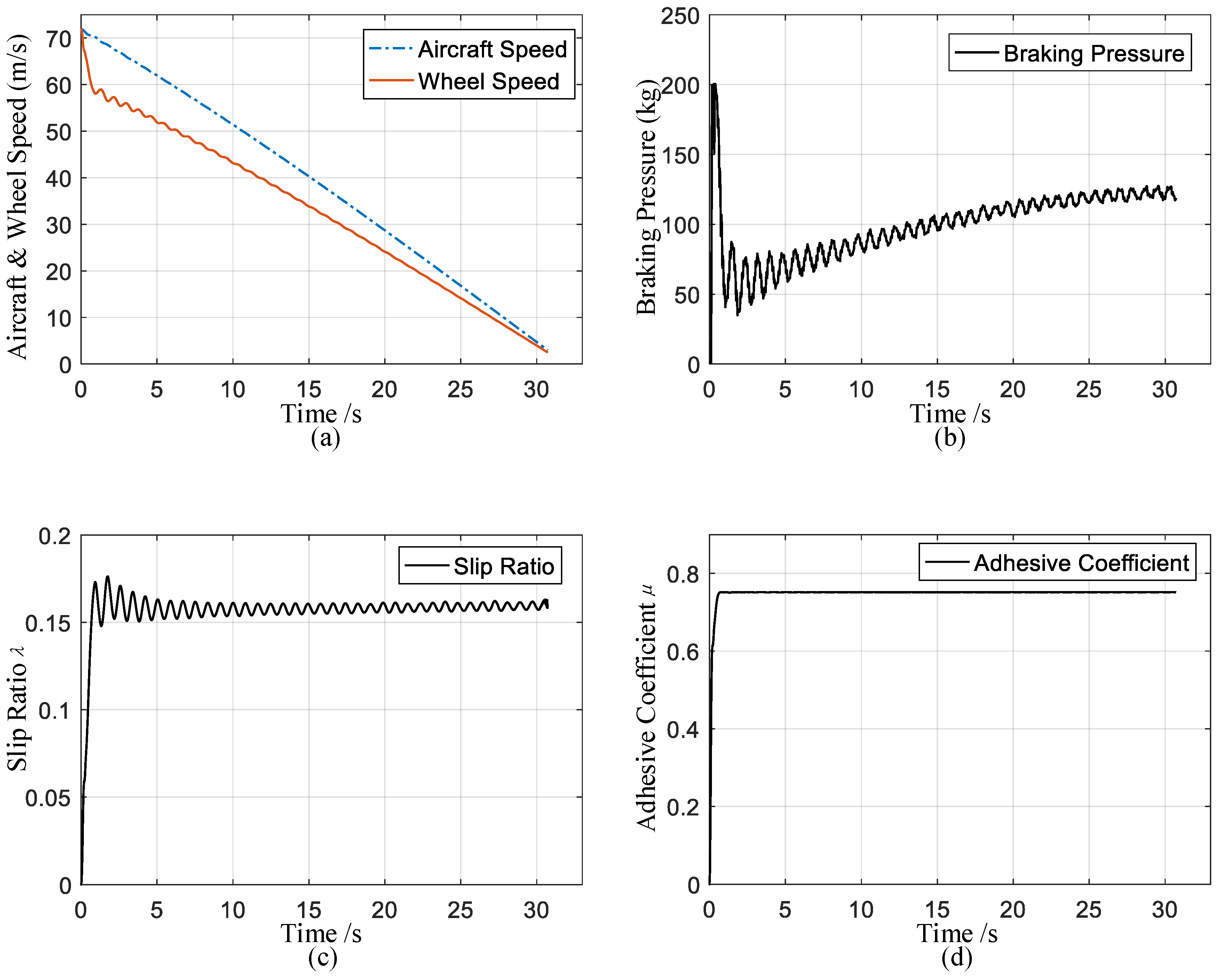
The initial conditions of the aircraft speed and the wheel speed are $V_x=72$ m/s and $V_w=72$ m/s, respectively. The limitation of the maximum braking pressure in the EMA controller is set at 225 kg. In the u-y function, the optimal wheel slip ratio is $\lambda =0.16$ and the maximum adhesive coefficient is $\mu =0.75$. All of the experimental data are saved by the upper computer and drawn by MATLAB.

The HIL experimental results are shown in Figure 7a–d. It can be clearly observed that the aircraft speed and wheel speed descend steadily under the action of the braking pressure. After a short time transient, the optimal slip ratio is well tracked and the corresponding adhesive coefficient remains stable around its maximum value without significant overshoots, which means that the proposed EMA controller can meet the requirements of the aircraft braking system.

5. Conclusions

Based on the analysis of the electric braking system, the ideal mathematical model of the EMA is established and the deformation of the reduction gear is analyzed. Then, the actual mathematical model is obtained by reasonably simplifying the nonlinear factors. A new RBF neural network-based adaptive backstepping design principle is adopted to address the multiple dynamics in the electric braking system. The Lyapunov function analysis indicates that the proposed control strategy guaranteed that the tracking error of braking pressure is uniformly ultimately bounded. The experimental results show that the servo performance of the EMA is improved significantly with the proposed control strategy compared with the traditional controller. Furthermore, the experimental results of the HIL test show that the performance of the proposed EMA controller can meet the requirements of the aircraft antilock braking system.