1. Introduction
In the past decade, due to the massive growth of data through various application domains, such as social media, mobile computing, and the Internet of Things (IoT), MapReduce [
1] has emerged as a highly successful framework for distributed and parallel computing on cloud systems. MapReduce allows the user to build complex computations on the data without having to worry about synchronization, fault tolerance, reliability or availability. Due to its simplicity, MapReduce has been widely used in various applications domains, such as search engine, database operations, machine learning, scientific computations, etc.
In particular, a MapReduce job runs in two main phases: Map and Reduce. In the Map phase, a master node splits the input dataset into independent smaller sub-tasks, and distributes them to worker nodes. Then, a worker node processes its sub-tasks in a parallel way and passes the intermediate result back to the master node. In the reduce phase, the master node distributes the intermediate data to the workers according to a partition function. Finally, the workers collect the intermediate data and combine them to form the final output for the original problem. This process allows MapReduce to process large data sets on distributed clusters.
The most popular open source implementation of MapReduce is Apache Hadoop. It was developed primarily by Yahoo and provides a distributed, scalable and portable file system, called HDFS, across clusters of computers. Both industry and academia, have adopted Apache Hadoop regularly to process and store large volumes of data [
2]. Although it is broadly used for large scale data processing, one of the major obstacles hindering effective processing on MapReduce is data skew. Data skew refers to unbalanced computational load, caused by the imbalance in the amount of data per tasks or by the imbalance in the amount of effort spent by workers to process the datasets. By default, Hadoop uses a hash function to determine the data partition corresponding to the reduce tasks. It works well when the data are uniformly distributed. However, in many real-world applications, the data partitioning method based on hash function results in a non-uniform distribution of the output data, and further leads to skewing of the input data in the reduce tasks. As a consequence, some worker nodes may be overloaded while others may be idle, affecting the performance in Hadoop MapReduce. This phenomenon is called Partitioning Skew.
Partitioning skew may occur naturally in many MapReduce applications. Bron-Kerbosch Clique [
3], for example, is an algorithm for finding maximal Cliques in a undirected graph. It can exhibit skew when a large Clique is being investigated. Another example is the Inverted Index, a data structure used for Web search that takes a list of documents as input and generates an inverted index for these documents. This structure can exhibit skew if a certain content appear in many more documents than others. A simple WordCount application can also produce this similar skew phenomena if a word appear many times within a text. Hence, guaranteeing a fair load balancing in the reduce phase of Hadoop MapReduce framework, considering data skew, is a valuable issue to be addressed.
In recent years, many studies have focused on the partitioning skew problem in MapReduce. Most of them [
4,
5,
6,
7,
8] acts at the intermediate data distribution and try to rebalance the key distribution among reduce tasks. However, in order to obtain the statistics related to the generated intermediate data, these solutions either wait for all the mappers to finish [
4,
5,
8] or add a sampling phase prior to the actual job start [
6,
7]. Thus, they lead to network overhead and I/O excessive costs. Skewtune [
9], a run-time skew mitigation technique, reallocates data that require more computational power to machines with more resources. Although this strategy improves performance of large data, it imposes high overhead, mainly on small amounts of data [
9]. Recently, some approaches [
2,
10,
11,
12] have been proposed by using prediction techniques to find the partition size even before the completion of the map tasks. These solutions dynamically allocate resources for reduce tasks according to their estimated value. Some of them adopt a linear regression-based prediction [
2,
12] and can achieve good accuracy only with the completion of a few mappers. However, predictions are inaccurate due to the data imbalance in the map phase. If the skew data occur only in the end of the map phase, or much later in the training model, the accuracy model will be affected, limiting their applicability.
Different from the previous work, we adopt metaheuristics to address the problem of how to efficiently partition the intermediate keys in the reduce phase of MapReduce framework, considering data skew. Our strategy aims to minimize an imbalance function that measures the load allocated to each machine by using three different metaheuristics: Simulated Annealing, Local Beam Search and Stochastic Beam Search. With metaheuristics, it is possible to guarantee fair distribution of the reducers’ inputs without prior knowledge about the data behavior and without explore the entire solution space. Thus, our strategy, called MAPSKEW, finds solutions close to the global optimum while having relatively small complexity. Additionally, it allows the user to set the tradeoff between performance and quality, based on metaheuristic parameters.
The main contributions of the paper are summarized below:
A novel approach to balance the workload among the reduce tasks, since the partitioning problem is NP-hard and our proposal finds, in polynomial time, good partitionings online, i.e., without needing to stop the execution of any phase of MapReduce.
A new partitioning method for general user-defined MapReduce programs. The method is highly adaptative since it uses metaheuristics, allowing the system manager to choose between performance and quality of the solution by adjusting hyperparameters.
An implementation of the proposed method in Hadoop 2.7.2 Yarn. Additionally, we have conducted several experiments with a real dataset, comparing the effects of different metaheuristics with related work and the native partitioning function of the Hadoop MapReduce on the Partitioning Skew.
2. Materials and Methods
2.1. MapReduce
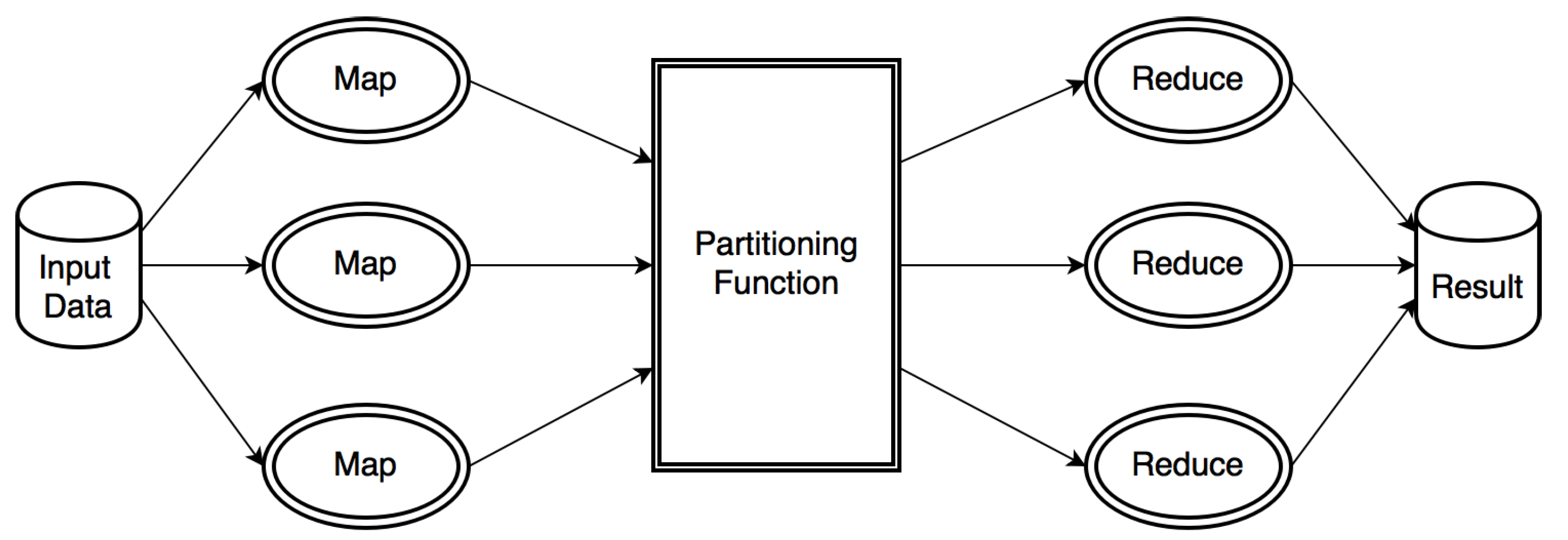
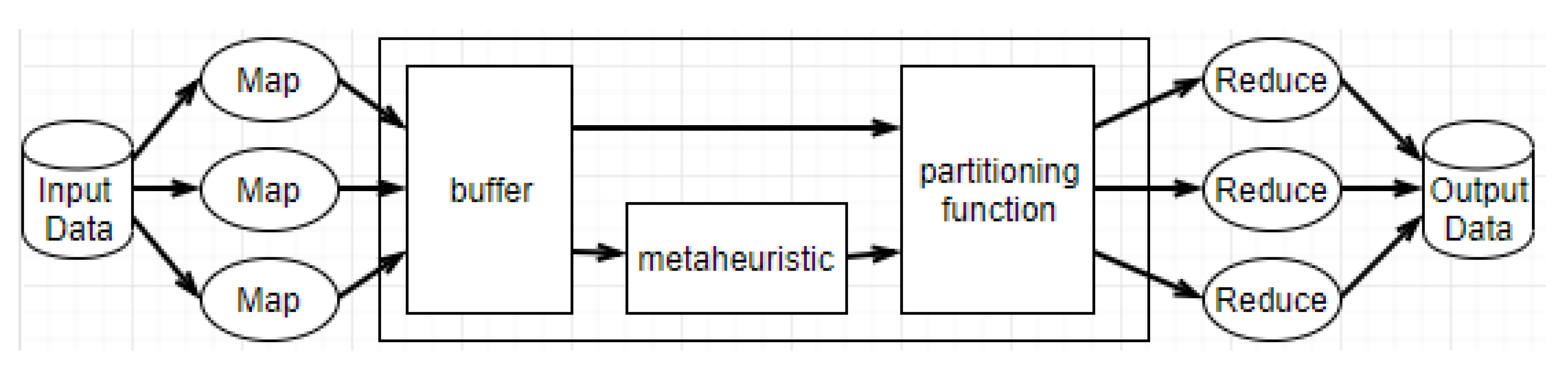
MapReduce is a framework introduced by Google for distributed and parallel computing on cloud environments. It was designed to handle large data volumes and huge clusters and to simplify synchronization, fault-tolerance, and scalability details from the application developer. MapReduce can significantly reduce the processing time of a large amount of data by dividing these data into smaller parts and processing them in parallel by multiple machines as shown in
Figure 1. It consists of two important phases, namely Map and Reduce. In the Map phase, input data is processed according to some user defined map function. After that, the framework generates a sequence of intermediate
pairs and a partitioning function is used to divide the data into multiple partitions, according to their keys, and allocate them across reduce tasks. This process is called Shuffle. By default, the partition function adopted is
R, where R is the number of reduce tasks.
Implementations of MapReduce framework have been written in different programming languages [
13,
14,
15]. Apache Hadoop is the most popular open source implementation of MapReduce.
2.2. Partitioning Skew
Currently, in MapReduce implementations, data are allocated to the reduce nodes according to the following
function:
where
is an integer associated with the key of an intermediary pair and
is the number of reduce nodes.
Usually, the
function allocates tasks so that the partitions get balanced. When the size of the key-value pairs is not uniformly distributed, the allocation of tasks becomes unbalanced. This type of situation characterizes partitioning skew, in which some reduce nodes receive high loads, increasing the time of response of assigned tasks, and others receive low loads, being idle because they have more resources allocated than necessary. Many authors studied the partitioning skew in mapreduce applications [
16,
17,
18,
19].
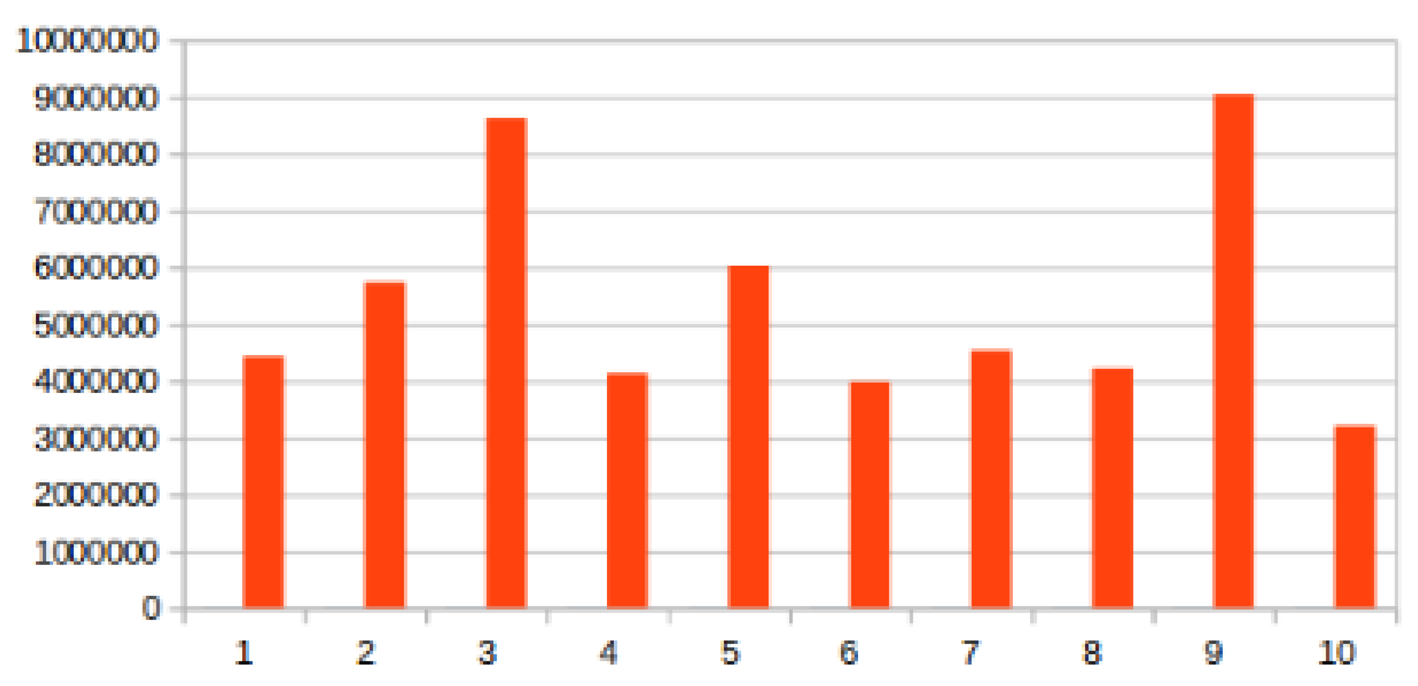
2.2.1. Skewed Key Frequencies
For several applications, some keys occur more frequently in the intermediate data. For example, in word count application some words appear more frequently than others, such as definite articles. In this type of application, the default Hadoop partitioning function will allocate tasks overloading the reduce nodes that receive most keys.
We present the size of ten different partitions measured by the sum of the size of each key of each partition in
Figure 2, this illustrates the partitioning skew generated by skewed key frequencies. As shown, partitions 3 and 9 either receive more keys or bigger keys than the remaining 8 partitions and, assuming a linear execution time, partition 10 would finish before the larger partitions reach their first half.
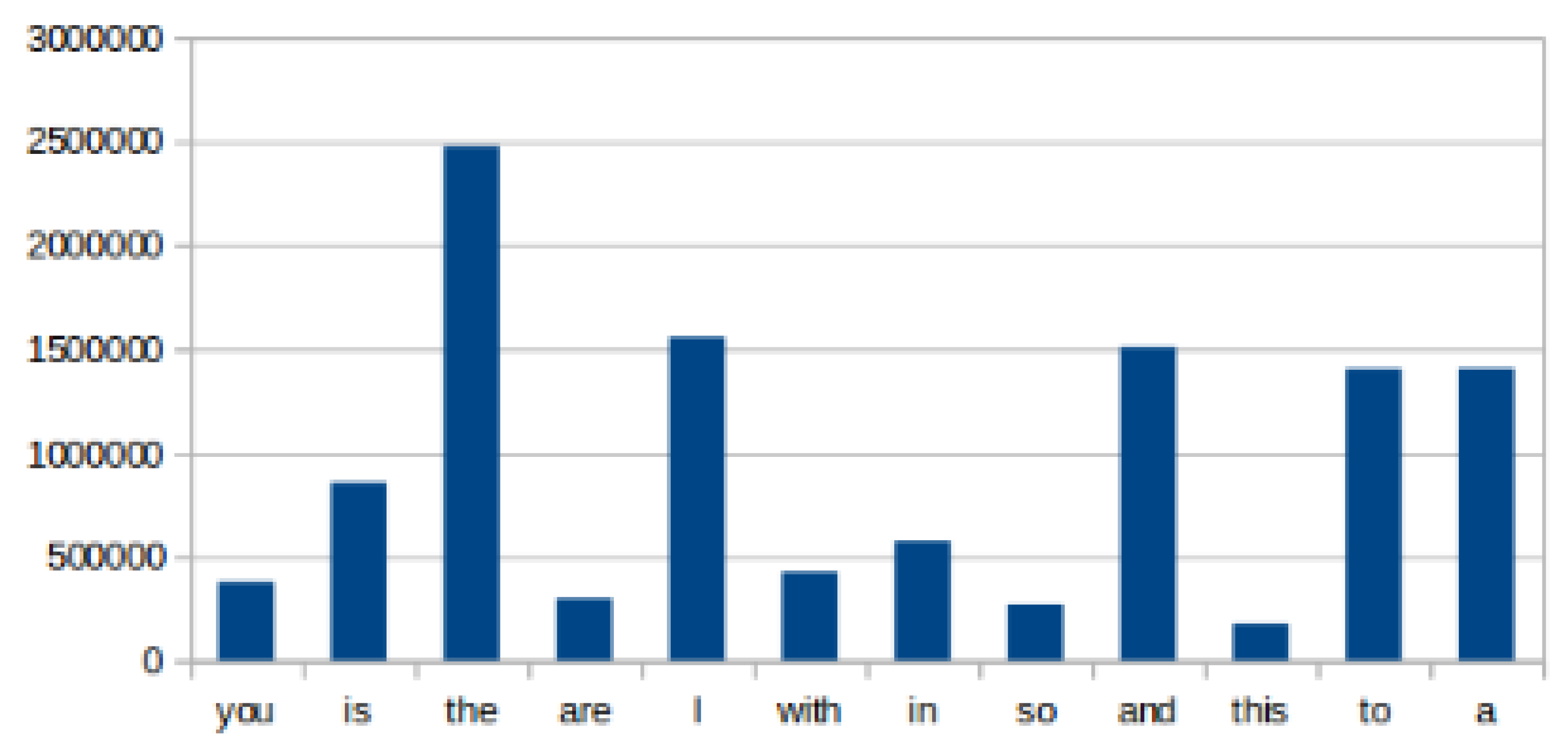
2.2.2. Skewed Key Sizes
In applications where value sizes in key-value pairs vary significantly, the distribution of the tasks to reduce nodes may become unbalanced. Thus, although the number of different values for each key is approximately the same, the execution time may vary between one key and another, resulting in some idle nodes while others are overloaded.
In
Figure 3, we present the biggest key from each partition shown in the previous figure as well as the following second and third biggest key from partition nine represented by the last two words, their size is measured by how many times they appear. Although the biggest key from the ninth partition is not as big as the key from the third, it alone is the greater than the sum of the smaller ones. Along with an already large key, other two equally large ones contribute to unbalance the partitions. If those larger keys where to be separated it would greatly benefit the load distribution.
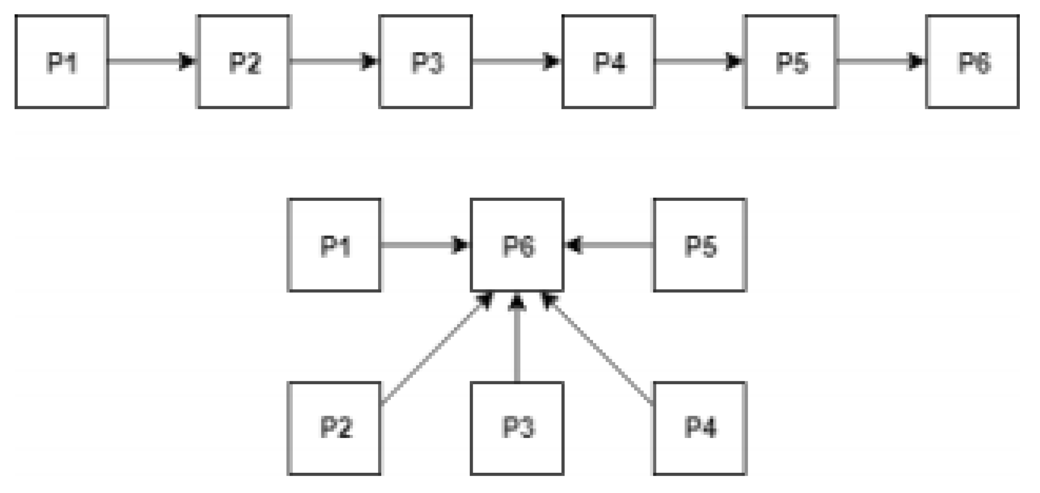
2.2.3. Skewed Execution Times
Some tasks may require more computing power than others. An example where this can occur is in the page classification algorithm that classifies a page according to the links to other pages, which we call neighboring pages. The greater the number of neighbors pointing to the same page, the longer it will take to process it.
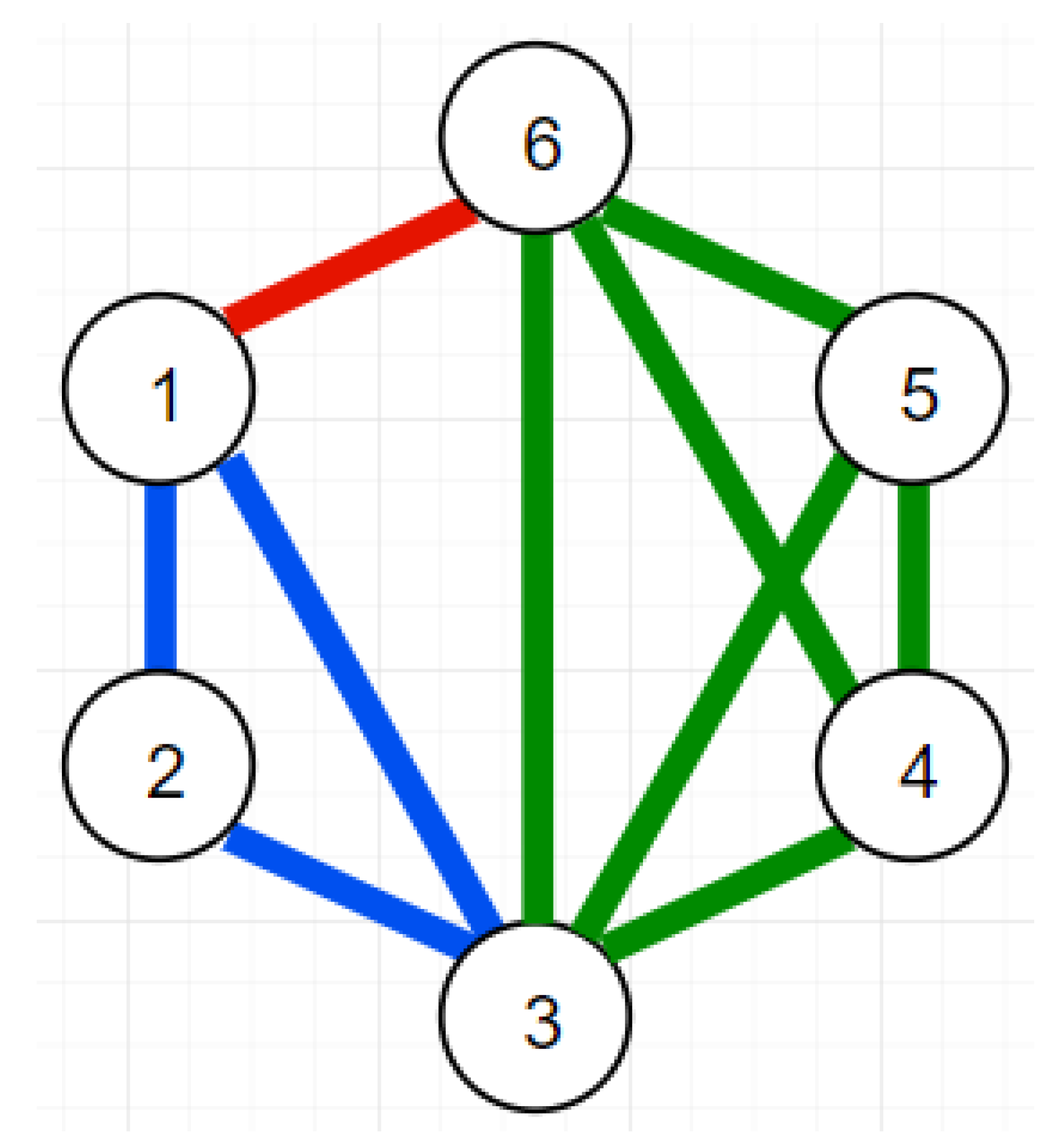
Figure 4 shows two simple example of a page rank execution where page 6 is reached by the same pages. In the first example, page 1 must pass through all other pages to reach page 6 meaning their distance is five. In the second example, all pages are directly linked to page 6 meaning their distance is one. In the end, example one is computationally heavier than example 2 since it need to check all links from each page to find the path that links page 1 to page 6.
2.3. Metaheuristics
Our main problem is to balance the load of the partitions to the reduce phase in search of an optimal configuration. A general solution for an optimization problem consists in exploring a (sub)set of solutions in order to find among them one that approximates the global optimum. Sometimes, like in the partitioning problem, the solution search space is very large and finding the global optimum by verifying every candidate solution takes an impracticable amount of time. In this context, metaheuristics may be used to find a good solution in a polynomial amount of time by searching a sample of the solution set.
In a metaheuristic, we look for a solution from small variations of a candidate solution, which can be generated in a random way. This variation is compared with the candidate solution for evaluation according to some criterion of acceptance. The best evaluated solution is maintained and the process is repeated until a stopping criterion is satisfied.
2.3.1. Simulated Annealing
In metallurgy, annealing is a process for hardening metals or glass by heating and cooling them gradually, allowing the material to reach a low-energy crystalline state [
20]. Simulated Annealing (SA) can be seen as the process of making a ping-pong ball reach the bottom of an irregular surface. If we just let the ball roll, it can get stuck at a point other than the bottom, because the surface is uneven. In order to the ball to leave the current point and continue rolling, it is necessary for someone to shake the surface.
In our problem, we want to attenuate the imbalance of the intermediate data allocated to the reducers. The solution based on SA is done as follows. An initial temperature and a cooling factor are defined. According to the intermediate data given as input, a key partitioning is created using the standard Hadoop partitioning function. We call this partitioning current partitioning. From this, we compare the current with a randomly generated neighbor partitioning. If the neighboring partitioning better balances the intermediate data allocated to each reducer, it becomes the current partitioning. Otherwise, the neighboring partitioning will become the current partitioning with a probability less than 1. This probability decreases proportionally to the current temperature. Finally, the current temperature is updated according to the cooling factor. This process is repeated until the temperature reaches 0. To facilitate understanding, we will show the pseudocode of this procedure.
In the Algorithm 1, we aim to reduce the imbalance, which is the load of the reducer with the highest volume of data allocated. That is, in order to balance the load, we must partition the keys between the reducers so that the allocated load of the machine with the highest allocation is minimal.
Our implementation consists of integrating Simulated Annealing to Hadoop, using it as the partitioning function. The partitioning phase works as follows: as the dataset is processed and the intermediate data is generated, Hadoop accumulates a portion of that data and the SA algorithm is executed to find an allocation that minimizes the unbalance of the reducers. This process will repeat itself until the end of the map phase.
| Algorithm 1 Simulated Annealing |
1: procedure Partitioner(D,T,C,R)
2: partitioning of the keys of D using .
3:
4:
5: while do
6:
7:
8:
9: if then
10:
11: else if then
12:
13:
14: return |
2.3.2. Local Beam Search
While in Simulated Annealing only one partitioning candidate is maintained, Local Beam Search (LBS) maintains k partitions, using more computing resources while covering a larger number of candidate solutions.
Intuitively, LBS acts as a group search, which group members divide through space in order to find an object. When one of the members suspects that he is close to the object, he calls the others to search in his area. Formally, the algorithm starts by generating a key partitioning is created using the standard Hadoop partitioning function, according to the intermediate data provided as input. Then, the algorithm generates random neighbors of the initial partitioning and selects among those the k partitions that present less imbalance. The partitions selected in the previous step will be called current partitions. From this, the algorithm will generate a random neighbor for each of the current partitions and will select k partitions that present less imbalance among current and generated partitions. The current partitions will be updated as the k partitions selected in the previous step. This process is repeated until a maximum number of iterations is reached. Then, the most balanced partitioning will be chosen. The pseudocode of this procedure is presented in Algorithm 2.
| Algorithm 2 Local Beam Search |
1: procedure Partitioner(k,D,I,R)
2: partitioning of the keys of D using .
3: createArray()
4: createArray()
5: for to do
6:
7:
8:
9: while do
10:
11:
12: for to k do
13:
14:
15:
16: return |
2.3.3. Stochastic Beam Search
In some situations, Local Beam Search can focus the search on a particular region of the solution space and get stuck in a local optima. A variation of Local Beam Search is Stochastic Beam Search, which reduces the possibility of occurring this kind of problem. Instead of choosing the k best partitions in terms of intermediate data balancing, Stochastic Beam Search chooses k partitions at random, with the most balanced partitions having most chances of being chosen. The pseudocode is presented in Algorithm 3.
| Algorithm 3 Stochastic Beam Search |
1: procedure Partitioner(k,D,I,R)
2: partitioning of the keys of D using .
3: createArray()
4: createArray()
5: for to do
6:
7:
8:
9: while do
10:
11:
12: for to k do
13:
14:
15:
16: return |
2.4. Bron-Kerbosch Clique
The Bron-Kerbosch Clique [
3] is a problem where, given an initial graph, the algorithm returns the biggest sub-graphs where all nodes are connected with one another. As an example of
Figure 5, nodes 1, 2 and 3 form a Clique, as well as nodes 1, 3 and 6, nodes 4, 5 and 6, and nodes 3, 4 and 5. Furthermore, the nodes 3, 4, 5 and 6 form a bigger Clique. We choose Clique due to its NP-completeness, which means that worst results are expected in skewed scenarios. The more complex the reduction function is, the more important it is to avoid placing large keys on the same partition.
2.5. Problem Definition
As previously discussed in
Section 2.1, MapReduce is a parallel computational model composed of a set of machines to process large amounts of data by its division between the machines. However, the division of the data may entail an unbalanced partitioning, also known as the partitioning skew. This problem has many several causes. Among them, we highlight the skewed key frequencies, the kewed key sizes and the skewed execution times. Except for the skew caused by the processing time of each key, which depends on the complexity of the reduce function, the data skew problem in MapReduce architectures can be addressed through of the data balancing between the cluster machines. The following definition will present the problem of finding an optimal partitioning as an optimization problem.
Definition 1. Optimal partitioning of a dataset
Let:
C A cluster of machines.
D A dataset.
a pair consisting of a key k and a value v obtained from D.
a partition consisting of a set of pairs t.
a partitioning of D where n is the number of partitions.
a function that returns the size of a partition. The size of the partition is equal to its cardinality.
a function that returns the unbalance of a partitioning P. The unbalance of P is defined as the biggest difference of the sizes of a pair of partitions in P.
the set of possible partitionings of D in n partitions.
is the optimal partitioning of D if and only if , , i.e., is the partitioning with the smallest unbalance among all partitionings of R.
As we have a definition of an optimal partitioning of a dataset, we can find it by searching the one with the smallest unbalance among the set of all possible partitionings. Although this method ensures the optimal partitioning, it is computationally expensive, since the number of partitionings of a dataset is exponential regarding its cardinality. Another method for finding the optimal partitioning is to use a greedy algorithm to find the smallest partition , such that , , in the moment that every element of the dataset arrives at the system. However, this method may fail to achieve good results depending on the order that the data is allocated to the partitions.
Before presenting the method proposed in this work, we will show the definition of neighboring partitions.
Definition 2. Neighboring Partitions.
Let two partitions. and are neighboring partitions if and only if they differ by the allocation of only one key or the exchange of the allocation of two keys, i.e., they are identical except for a key k such that in and in or they are identical except for the keys such that , in and , in .
Please note that a possible solution for finding the optimal partitioning lays in creating a random partitioning P and verifying if one of its neighboring partitionings has a better balancing than P and repeat this process using as the initial partitioning. This process may be repeated a finite number of iterations in order to find a good partitioning. This strategy is similar to the execution of the Hill Climbing metaheuristic. Although this process may return good partitionings, it may return local optima results depending on the initial partitioning.
Our strategy, named MAPSkew, is a metaheuristic-based approach for online load balancing in MapReduce environments with skewed data. MAPSkew works in the shuffle phase, accumulating a percentage of the input data processed by the map phase and executing a metaheuristic for finding a partitioning over this accumulated data searching for minimizing the unbalancing defined in Definition 1. This process is repeated respecting the key already allocated until all the input data is processed. The
Figure 6 shows the architecture of MAPSkew.
Our changes in Hadoop core consist of the addition of data structures to hold the additional information required by the metaheuristics as well as their code. The parameters passing is made by an extra archive read by the system when a job is launched. Our compiled version of hadoop can be found through the Dropbox service [
21].
2.6. Tests Setup and Comparisons
Our experiments have been performed on one master and nine worker processing nodes, each one with 16 GB of RAM, 16 virtualized CPUs, and 160 GB of permanent storage. All virtual machines are running in an OpenStack cloud environment hosted at the LSBD/UFC. We have executed a Bron-Kerbosch Clique application over a modified version of Facebook egonets dataset [
22] made up of a series of nodes and edges, forming a graph of integers. To force data skew, we have selected a set of random nodes whose hash key value are sent to a predetermined partition. We have decided to build an artificial skewed dataset because the original data set is originally balanced, which would remove the need for a new partitioning process. The number of nodes in our skewed dataset is 1000. Combined with the complexity of the Bron-Kerbosch algorithm, this is enough to create a sufficiently complex scenario for our experiments.
For the performance evaluation, we varied the hyper-parameters of the metaheuristics by changing the number of iterations (1000, 3000 and 5000 iterations) and the number of simultaneous candidate solutions (1, 5, 9 simultaneous candidates). Please note that the last hyperparameter is not used in the Simulated Annealing. Furthermore, our method uses an extra parameter that defines the amount of data that is accumulated at every execution of the selected metaheuristic. In percentages of the input data, such a parameter may assume the following values: 5%, 10%, 20% and 30%. The total number of experiments, taking into consideration the three metaheuristics and their respective hyperparameters, is 85. Each experiment was repeated 5 times in order to remove outliers and other random factors that may interfere with the execution.
3. Results and Discussion
3.1. Balancing
As shown in
Table 1, the metaheuristics reduced the skew by up to
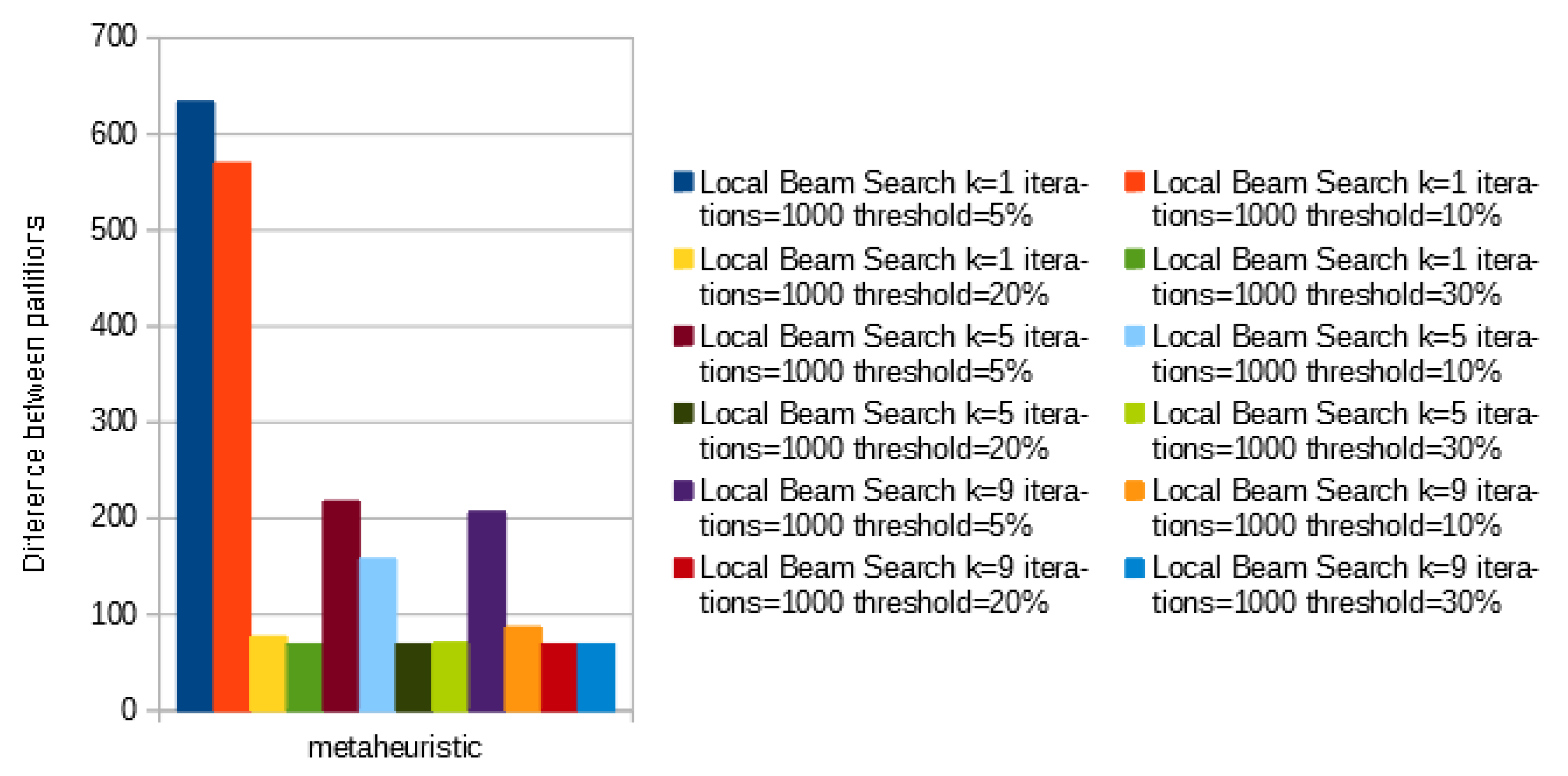
. Local and Stochastic Beam Search Achieved great results with threshold percentage being a major factor while K and temperature being not so relevant at a first sight. To improve our investigation about the most relevant attribute, in
Figure 7 we set the number of iterations to 1000 and analyze the threshold and number of candidates per iterations. Every time the threshold reach 20% the difference between partitions suffers a huge drop, especially when only one candidate is selected per iteration.
In terms of balancing, Simulated Annealing achieved the worst results among the three metaheuristics, as shown in
Table 2. The configuration with the best result, representing about
decrease in partitions size, is slightly worse than the worst result of Stochastic Beam Search. However, the worst result of the metaheuristics is still better than the base hash partitioning method, meaning that even the slightly change may help reduce the existent skew. It is important to notice that the Simulated Annealing configurations with a threshold of
or
achieved better results than the ones with a threshold of
or
.
It is clear that, in terms of skewness reduction, the size of the threshold is more important than the number of iterations or the number of candidates per iteration (K). Furthermore, it would be possible to test with even less iterations to reduce the overhead in this particular scenario, although it does not seem to be necessary. It would also be interesting to try other threshold values between and to see how those would fare in the table.
Local Beam Search performs better than Stochastic Beam Search when tested with a sufficient large threshold percentage and enough number of iterations. Contrariwise, Local Beam Search seems to perform worse than Stochastic Beam Search when tested with small Threshold percentage and small K. This can conclude that: with a sufficient number of iterations and a sufficient number of accumulated keys, Local Beam Search is not impaired by a small number of candidates per iteration. However, when we reduce the number of accumulated keys in our threshold, the number of candidates per iteration becomes more important than the number of iterations, since it represents the number of possible paths within each step.
The same observations of Local Beam Search are valid to Stochastic Beam Search. In addition to what has been already pointed out, Stochastic Beam Search seems to perform a little more consistently than Local Beam Search, presenting itself as a more reliable alternative when focusing in partitioning. Simulated Annealing, however, has not been performed well in this experiments. This behavior may have been caused by the fact that it always select only one path per iteration. This, in case of a bad choice, it will keep that bad choice, without much alternatives to work around.
3.2. Time
Table 3 shows the ten best and the ten worst execution times across configurations. Firstly, it can be noticed that even in the worst case, metaheuristic configurations are fast than the base hash. However, we may not conclude what attribute(s) mostly contributes to the improvement in execution time, since all ranges of metaheuristics and hyperparameters can be found among the best and the worst results. We think this can be explained by the NP-completeness of Bron-Kerbosch Clique, so that the keys do not follow a rule to determine the time spent with each clique search. Furthermore, the improvement in execution time seems to be caused more by the separation of large keys than by the balancing itself.
As an extension to the metaheuristics, it would be possible to assign another weight calculation to the keys as a way to give more importance to larger keys and decrease the chances of two large keys being allocated on the same partition. Since these keys are responsible for most of time spent during processing, it is crucial to handle them with special care during partitioning.
4. Conclusions
In this paper, we have presented a solution to mitigate the skew problem originated in the reduce phase of MapReduce computations, by better distributing the keys to the partitions and improving the time by separating large keys. As long as the partitioning keep being left as secondary, skewed data will keep being a problem in terms of optimization and load management. The research works reported in the literature often address this problem with a previous knowledge about the key distribution, gathered in past executions. Another approach is to reallocate the load during the reduction phase. Our approach works during the map phase together with the system, in order to allocate the data in the best possible way. Although an optimal allocation is preferred, our approach attempts to deliver a good distribution without being necessary to wait for all keys to be processed before the partitioning.
As discussed in
Section 3, the experimental evaluation has shown that the accumulated threshold percentage is the leading factor for a good balancing. Moreover, the number of candidates per iteration is only relevant when the threshold is small, and the number of iterations is highly dependant of the total size of the problem. Furthermore, there are still numerous configurations, as well as other algorithms, which we can use to analyze the impact of skew and skew reduction. We have noticed that the more complex the function, the better it is to test our solution.
To reach an optimal number of iterations, we are planning a model based on percentage instead of setting a fixed number. Such a dynamic approach would avoid unnecessary iterations, which would increase the overhead caused by partitioning. Also, for further works, we discussed the idea of a weight system mentioned in
Section 3.2. We plan to keep refining our solution until we are satisfied with how it can interact with the system. Finally, other further works include automatizing the selection of parameters and a possible data pre-partitioning to accelerate the shuffle phase.

