Robust Guaranteed-Cost Preview Repetitive Control for Polytopic Uncertain Discrete-Time Systems ^†

Abstract

In this paper, a robust guaranteed-cost preview repetitive controller is proposed for a class of polytopic uncertain discrete-time systems. In order to improve the tracking performance, a repetitive controller, combined with preview compensator, is inserted in the forward channel. By using the L-order forward difference operator, an augmented dynamic system is constructed. Then, the guaranteed-cost preview repetitive control problem is transformed into a guaranteed-cost control problem for the augmented dynamic system. For a given performance index, the sufficient condition of asymptotic stability for the closed-loop system is derived by using a parameter-dependent Lyapunov function method and linear matrix inequality (LMI) techniques. Incorporating the controller obtained into the original system, the guaranteed-cost preview repetitive controller is derived. A numerical example is also included, to show the effectiveness of the proposed method.

1. Introduction

In some control systems, it is hoped that the output can track the reference signal without steady-state error, even in the presence of uncertainty and/or exogenous disturbances. Preview control [1,2] is one of the many ways to solve this kind of control problem. The basic idea of preview control is to use known future information of the reference or disturbance signals. It was found that preview control can enhance performance of the closed-loop system [3]. In recent years, the problem of preview control has received considerable attention and various control structures and algorithms have been proposed [4,5,6,7].

As a typical regulator method, the linear quadratic regulator optimal control is a powerful technique for designing preview controllers [8,9,10]. In [8], a preview-based linear quadratic design method was investigated for reference-tracking motion control. In this way, the explicit implementation formulas for feedforward controllers were derived that can be applied to a range of rigid-body motion systems. In [9], a preview control using a feedforward-imperfect forecast measurement of a disturbance signal was proposed, in the context of discrete-time linear quadratic Gaussian control. In [10], the constrained optimal preview control of dual-stage actuators was proposed, and the problem was solved in terms of quadratic programming. In [11], using the reference and disturbance signal preview information, an optimal feed-forward preview controller was presented for single-input single-output systems. In order to estimate the unmeasurable state vector, a state observer-based optimal preview controller was developed in [12]. Other relevant work may refer to [13]. However, as well known, the classical LQR-based optimal preview control cannot be directly applied to uncertain systems.

For uncertain systems, it will become difficult to design preview controller. In [14], a robust tracking problem for a polytopic uncertain system subject to a previewable reference signal was considered. In [15], a linear matrix inequality (LMI)-based robust preview tracking problems for discrete systems with polytopic uncertainties was provided. In [16], the problem of multi-model adaptive preview control was proposed for discrete-time systems with unknown piecewise constant coefficients. In [17], the author overviewed the preview control research achievements and discussed the main existing problems. Very recently, for a class of polytopic uncertain discrete systems, by combining parameter-dependent Lyapunov function method with LMI techniques, a static output feedback preview tracking controller was presented in [18]. For a class of uncertain discrete-time systems, an LMI-based preview controller was proposed in [19]. The proposed method can be extended completely to preview control for time varying systems.

Repetitive control (RC), which was first developed in the early 1980s [20], is a very useful strategy for tracking periodic reference signals [21,22,23]. Although the repetitive control method was originally proposed in continuous-time systems, it was realized by a digital computer in the actual applications. The direct design of a repetitive controller in the discrete time domain is of practical significance. In [24], a discrete-time variable-structure repetitive control was proposed. The presented control scheme ensures robust stability of the resultant quasi-sliding-mode dynamics to parameter variations and exogenous disturbances. The authors in [25] have investigated a positive realness problem, raised in discrete repetitive control. The sufficient condition of the repetitive control stability can be satisfied through constructing a discrete positive real transfer function. Based on two-dimensional system theory, the problem of designing discrete-time repetitive-control systems was studied in [26,27]. By the same argument, the observer-based repetitive controller design method for discrete-time systems with uncertainties was presented in [28]. Iterative learning control (ILC) [29] which imposes a special boundary condition on the system, is closely related to repetitive control. In the case of discrete linear dynamics, there are many methods for the ILC design. Recently, an innovative ILC law which was augmented by a state feedback controller with a dynamic feedforward controller was developed in [30,31]. The experimental results show that feedforward control can improve tracking accuracy significantly.

On the other hand, for many control systems, when a system is dependent on uncertain parameters it is desirable to design a control system that is not only asymptotically stable, but also guarantees an adequate level of control performance. This kind of control problem is called guaranteed-cost control [32,33]. For a class of uncertain discrete-time systems, a guaranteed-cost preview controller was proposed in [19]. For discrete-time linear systems with uncertainties, a method of designing a guaranteed-cost robust discrete repetitive controller based on two-dimensional model was proposed in [34]. For continuous-time linear systems, the design of non-fragile guaranteed-cost repetitive control was studied in [35]. It should be noted that guaranteed-cost preview repetitive control problems have not been considered, so far.

In this paper, motivated by the above results, a new configuration of repetitive control system with preview feedforward compensation, as well as the guaranteed-cost preview repetitive controller design method is presented. Using the lift technique, an augmented state-space dynamic system is constructed. The robust guaranteed-cost preview repetitive controller design problem is then transformed into the guaranteed-cost control problem of the augmented system. By combining a parameter-dependent Lyapunov function method with LMI techniques, the guaranteed-cost preview repetitive controller is obtained.

The rest of this paper is organized as follows: Section 2 presents the problem formulation and preliminaries. Section 3 describes the construction of an augmented dynamic system. The design of the guaranteed-cost preview repetitive controller is explained in Section 4. Section 5 presents a numerical example, to demonstrate the effectiveness of the method. Finally, Section 6 gives some concluding remarks.

Throughout this paper, ${\mathbb{R}}^n$ denotes n-dimensional Euclidean space, ${\mathbb{R}}^{n\times m}$ is the set of all $n\times m$ real matrices, I is the identity matrix of appropriate order, $0_{p\times p}$ is the $p\times p$ zero matrix (the subscript is omitted, if the dimension is clear), and ∗ indicates the entries below the main diagonal of a symmetric block matrix. The notation $X>0(<0)$ means that matrix X is positive (negative) definite.

2. Problem Formulation and Preliminaries

Consider the following uncertain SISO discrete-time system:

$$\left\{\begin{array}{c}x(k+1)=A\left(\theta \right)x\left(k\right)+B\left(\theta \right)u\left(k\right)+Ed\left(k\right),\hfill \\ y\left(k\right)=Cx\left(k\right),\hfill \end{array}\right.$$

(1)

where $x\left(k\right)\in {\mathbb{R}}^n$ is the state, $u\left(k\right)\in {\mathbb{R}}^m$ is the control input, $d\left(k\right)\in {\mathbb{R}}^p$ is the periodic disturbance, and $y\left(k\right)\in {\mathbb{R}}^q$ is the output of the plant. E and C are constant matrices with appropriate dimensions. $A\left(\theta \right)$ and $B\left(\theta \right)$ are uncertain matrices with appropriate dimensions, and are given by

$$\left[A\left(\theta \right)B\left(\theta \right)\right]={\displaystyle \sum _{i=1}^s}{\theta }_i\left[A_i{B}_i\right],$$

(2)

where $A_i$ and $B_i$, $(i=1,2,\dots ,s)$, are constant matrices with appropriate dimensions, and $\theta ={[{\theta }_1,{\theta }_2,\dots ,{\theta }_s]}^T$ is the uncertain constant parameter vector satisfying

$$\theta \in \mathrm{\Theta }:=\left\{\theta \in {\mathbb{R}}^s|{\theta }_i\ge 0,(i=1,2,\dots ,s),{\displaystyle \sum _{i=1}^s}{\theta }_i=1\right\}.$$

(3)

Let $r\left(k\right)\in {\mathbb{R}}^q$ be a periodic reference signal to be tracked by $y\left(k\right)\in {\mathbb{R}}^q$, and

$$e\left(k\right)=r\left(k\right)-y\left(k\right)$$

(4)

be the tracking error.

Throughout this paper, two assumptions are made:

A1: The reference signal $r\left(k\right)$ and disturbance signal $d\left(k\right)$ are periodic, both of period L.

A2: The preview lengths of the reference signal $r\left(k\right)$ and disturbance signal $d\left(k\right)$ are $M_r$ and $M_d$ ($M_r,M_d$ are less than L), respectively. That is, at each time k, the $M_r$ ($M_d$) future values, $r(k+1)$, $r(k+2)$, …, $r(k+M_r)$ ($d(k+1)$, $d(k+2)$, …, $d(k+M_d)$), as well as the present and past values of the reference signal, are available.

Remark 1.

In fact, the disturbance signal and the reference signal are not necessarily the same period. In this case, the period of the repetitive controller can be set as the minimum common multiple of the period of reference signal and interference signal.

Remark 2.

Assumption A2 implies that the reference and the disturbance signals are previewable. Conventional discrete-time feedback control systems and the dynamic feedforward control scheme do not take full advantage of the known future values; that is, $M_r=0$ and $M_d=0$. Moreover, assumption A2 indicates that the previewable reference and the disturbance signals have significantly impacted performance in the control system only for a certain time period, during which the reference signal exceeds the preview length, and the impact is very small [2,4,5].

Remark 3.

The future values of the disturbance signal are assumed to be measured in assumption A2. Admittedly, it is a very strong assumption. In most cases, the complete future disturbance signal cannot be measured directly. For some given control systems, the detailed mathematical modeling and estimation of future disturbance signal can refer to [36,37].

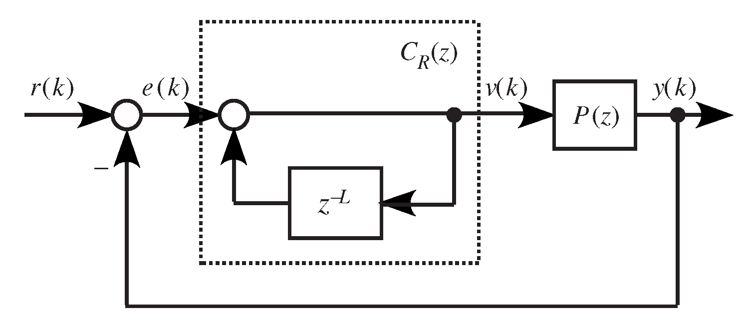
The basic configuration of a discrete-time repetitive control system [38] is shown in Figure 1, where $P\left(z\right)$ is the compensated plant, $r\left(k\right)$ is a periodic reference input with period L, and

$${\displaystyle C_R\left(z\right)=\frac{1}{1-z^{-L}}}$$

(5)

is a repetitive controller. The output of the repetitive controller, $v\left(k\right)$, is

$$v\left(k\right)=\left\{\begin{array}{cc}v(k-L)+e\left(k\right),\hfill & k\ge L,\hfill \\ e\left(k\right),\hfill & k<L.\hfill \end{array}\right.$$

(6)

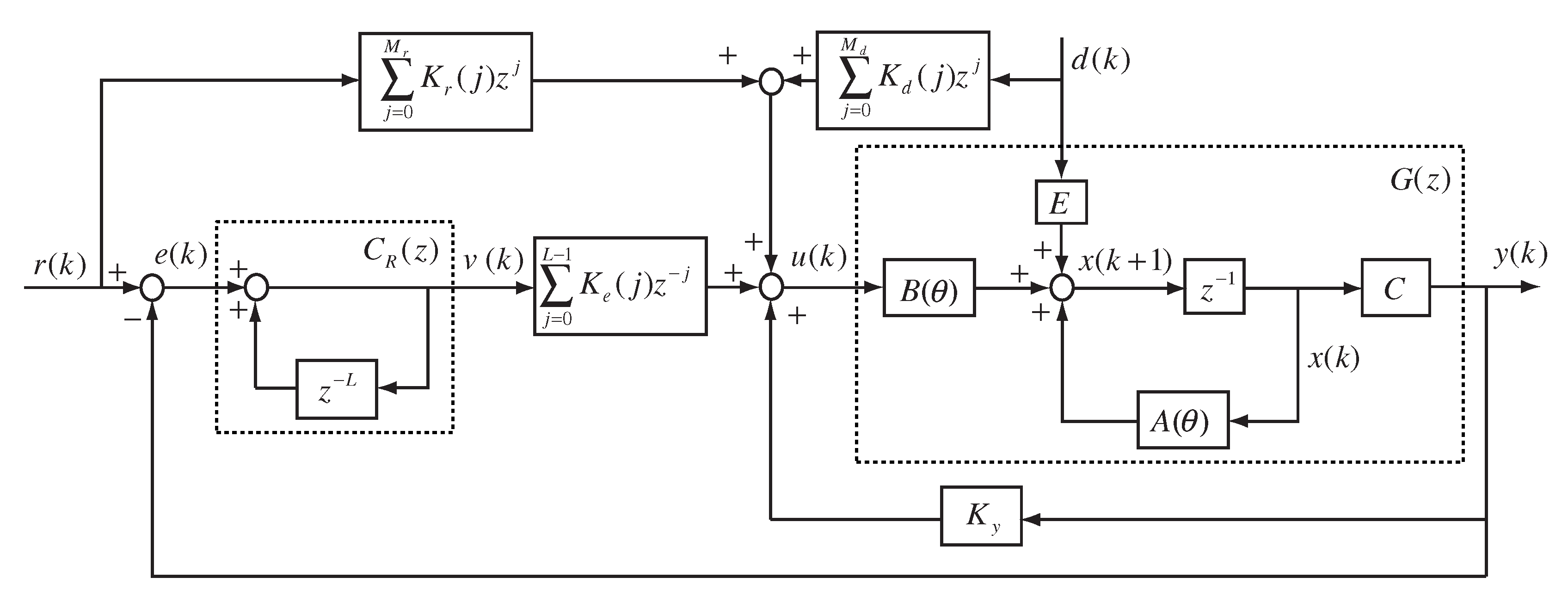
This paper concerns the repetitive-control system configuration in Figure 2, where $G\left(z\right)$ is the controlled plant as described in System (1). $K_r\left(j\right)$, $(j=0,1,2,\dots ,M_r)$, and $K_d\left(j\right)(j=0,1,2,\dots ,M_d)$ are the gains of the reference signal and disturbance signal preview compensator, respectively. $K_e\left(j\right)$, $(j=0,1,2,\dots ,L-1)$, and $K_y$ are the gains of the repetitive controller and the output feedback controller, respectively.

The objective is to design a guaranteed-cost preview control law, with the form

$$u\left(k\right)={\displaystyle \sum _{j=0}^{L-1}}{K}_e\left(j\right)v(k-j)+K_{y}y\left(k\right)+{\displaystyle \sum _{j=0}^{M_r}}{K}_r\left(j\right)r(k+j)+{\displaystyle \sum _{j=0}^{M_d}}{K}_d\left(j\right)d(k+j).$$

(7)

Remark 4.

The preview repetitive controller (7) consists of four parts: The first part is repetitive control, the second term represents output feedback, the third and the fourth represent the preview action based on the future values of the previewable reference signal and the disturbance signal. Besides, considering that the system states are not measurable, the static output feedback is used instead of taking the state feedback.

Remark 5.

Based on a state feedback controller with integral action and a dynamic feedforward controller, a new ILC structure was proposed in [31]. Similarly, the future values of the reference trajectory $r\left(k\right)$ and the integral of the learning action are contained in the preview repetitive controller (7), which can be viewed as a feedforward controller and help the system reduce static errors.

For an uncertain discrete-time system (1), we introduce a quadratic cost function

$$J={\displaystyle \sum _{k=0}^{\infty }}\left[e{\left(k\right)}^T{Q}_{e}e\left(k\right)+\Delta u{\left(k\right)}^{T}R\Delta u\left(k\right)\right],$$

(8)

where $\Delta u\left(k\right)=u\left(k\right)-u(k-L)$, $Q_e$, and R are the given symmetric, positive definite weighting matrices.

A guaranteed-cost preview controller is defined as follows.

Definition 1.

For the uncertain discrete-time system (1) and the cost function (8), if there exists a preview repetitive-control law (7) that produces a control input $u^{*}\left(k\right)$, a positive constant $J^{*}$ such that $\underset{k\to \infty }{lim}e\left(k\right)=0$, and, for all admissible uncertainties, the closed-loop system is robustly stable and the value of the cost function (8) satisfies $J\le J^{*}$, then $J^{*}$ is said to be a guaranteed cost and $u^{*}\left(k\right)$ is said to be a guaranteed-cost preview repetitive-controller for the cost function (8).

To obtain our main results, the following lemmas will be used.

Lemma 1

(Schur complement [39]). For a real matrix $\sum ={\sum }^T$, the following assertions are equivalent:

i. 

$\sum :=\left[\begin{array}{cc}{\sum }_{11}& {\sum }_{12}\\ ★& {\sum }_{22}\end{array}\right]>0.$

ii. 

${\sum }_{11}>0,\mathrm{and}{\sum }_{22}-{\sum }_{12}^T{\sum }_{11}^{-1}{\sum }_{12}>0.$

iii. 

${\sum }_{22}>0,\mathrm{and}{\sum }_{11}-{\sum }_{12}{\sum }_{22}^{-1}{\sum }_{12}^T>0.$

Lemma 2

([40]). For the matrices $L\in {\mathbb{R}}^{n\times n}$, $H\in {\mathbb{R}}^{n\times n}$, and $H>0$, one has

$$-L^T{H}^{-1}L\le -L-L^T+H.$$

(9)

Lemma 3

([41]). For appropriately dimensioned matrices T, S, R, N, and scalar β, $T+S^T{R}^T+RS<0$ if the following condition holds:

$$\left[\begin{array}{cc}T& {(\beta R^T+N{S}^T)}^T\\ \beta R^T+N{S}^T& -\beta N-\beta N^T\end{array}\right]<0.$$

(10)

3. Construction of Augmented Dynamic System

In this section, we will construct an augmented dynamic system that includes previewed information, error vectors, and states of the system by using the L-order forward difference operator. Moreover, the augmented performance index will be also given.

For all the system variables, define the L-order forward difference operator as

$$\Delta \xi \left(k\right)=\xi \left(k\right)-\xi (k-L),\xi \in \{x,y,u,r,d\}.$$

(11)

Taking the L-order difference operator on both sides of the state Equation (1) and error Equation (4), we derive

$$\left\{\begin{array}{c}e(k+1)=e(k+1-L)+\Delta r(k+1)-CA\left(\theta \right)\Delta x\left(k\right)\hfill \\ -CB\left(\theta \right)\Delta u\left(k\right)-CE\Delta d\left(k\right),\hfill \\ \Delta x(k+1)=A\left(\theta \right)\Delta x\left(k\right)+B\left(\theta \right)\Delta u\left(k\right)+E\Delta d\left(k\right),\hfill \\ \Delta y\left(k\right)=C\Delta x\left(k\right).\hfill \end{array}\right.$$

(12)

Defining

$$\left\{\begin{array}{c}{x}_e\left(k\right)={[e^T\left(k\right)e^T(k-1)\dots e^T(k-L+1)]}^T,\hfill \\ \overline{x}\left(k\right)={[x_e^T\left(k\right)\Delta x^T\left(k\right)]}^T,\hfill \end{array}\right.$$

(13)

and combining (12) and (13), we have

$$\overline{x}(k+1)=\overline{A}\left(\theta \right)\overline{x}\left(k\right)+\overline{B}\left(\theta \right)\Delta u\left(k\right)+G_r\Delta r(k+1)+G_d\Delta d\left(k\right),$$

(14)

where

$$\begin{array}{c}\overline{A}\left(\theta \right)=\left(\begin{array}{ccccc}0& \cdots & 0& I& -CA\left(\theta \right)\\ I& \cdots & 0& 0& 0\\ ⋮& ⋮& ⋮& ⋮\\ 0& \cdots & I& 0& 0\\ 0& \cdots & 0& 0& A\left(\theta \right)\end{array}\right),\hfill \\ \overline{B}\left(\theta \right)=\left(\begin{array}{c}-CB\left(\theta \right)\\ 0\\ ⋮\\ 0\\ B\left(\theta \right)\end{array}\right),G_r=\left(\begin{array}{c}I\\ 0\\ ⋮\\ 0\\ 0\end{array}\right),G_d=\left(\begin{array}{c}-CE\\ 0\\ ⋮\\ 0\\ E\end{array}\right).\hfill \end{array}$$

From (2), the uncertain matrices $\overline{A}\left(\theta \right)$ and $\overline{B}\left(\theta \right)$ can be rewritten as

$$\begin{array}{ll}\overline{A}\left(\theta \right)& =\left(\begin{array}{ccccc}0& \cdots & 0& I& -C{\displaystyle \sum _{i=1}^s}{\theta }_i{A}_i\\ I& \cdots & 0& 0& 0\\ ⋮& ⋮& ⋮& ⋮\\ 0& \cdots & I& 0& 0\\ 0& \cdots & 0& 0& {\displaystyle \sum _{i=1}^s}{\theta }_i{A}_i\end{array}\right)\\ & ={\displaystyle \sum _{i=1}^s}{\theta }_i\left(\begin{array}{ccccc}0& \cdots & 0& I& -C{A}_i\\ I& \cdots & 0& 0& 0\\ ⋮& ⋮& ⋮& ⋮\\ 0& \cdots & I& 0& 0\\ 0& \cdots & 0& 0& A_i\end{array}\right)={\displaystyle \sum _{i=1}^s}{\theta }_i{\overline{A}}_i,\end{array}$$

(15)

$$\overline{B}\left(\theta \right)=\left(\begin{array}{c}-C{\displaystyle \sum _{i=1}^s}{\theta }_i{B}_i\\ 0\\ ⋮\\ 0\\ {\displaystyle \sum _{i=1}^s}{\theta }_i{B}_i\end{array}\right)={\displaystyle \sum _{i=1}^s}{\theta }_i\left(\begin{array}{c}-C{B}_i\\ 0\\ ⋮\\ 0\\ B_i\end{array}\right)={\displaystyle \sum _{i=1}^s}{\theta }_i{\overline{B}}_i.$$

(16)

For the uncertain system (14), we specify the observation equation as

$$e\left(k\right)=\overline{C}\overline{x}\left(k\right),$$

(17)

where $\overline{C}=\left[I_q{0}_{q\times \left[\right(L-1)q+n]}\right].$

Defining

$$X_r\left(k\right)=\left(\begin{array}{c}\Delta r\left(k\right)\\ \Delta r(k+1)\\ ⋮\\ \Delta r(k+M_r)\end{array}\right),X_d\left(k\right)=\left(\begin{array}{c}\Delta r\left(k\right)\\ \Delta r(k+1)\\ ⋮\\ \Delta r(k+M_d)\end{array}\right),$$

(18)

it follows from assumptions A1 and A2 that $X_r\left(k\right),X_d\left(k\right)$ satisfy

$$X_r(k+1)=A_r{X}_r\left(k\right),$$

(19)

$$\begin{array}{c}\hfill X_d(k+1)=A_d{X}_d\left(k\right),\end{array}$$

(20)

where $A_r\in {\mathbb{R}}^{q(M_r+1)\times q(M_r+1)},A_d\in {\mathbb{R}}^{p(M_d+1)\times p(M_d+1)}$, and

$$A_r=\left(\begin{array}{ccccc}0& I& 0& \cdots & 0\\ 0& \ddots & \ddots & \ddots & ⋮\\ ⋮& \ddots & \ddots & 0\\ 0& \cdots & \cdots & 0& I\\ 0& \cdots & \cdots & 0& 0\end{array}\right),A_d=\left(\begin{array}{ccccc}0& I& 0& \cdots & 0\\ 0& \ddots & \ddots & \ddots & ⋮\\ ⋮& \ddots & \ddots & 0\\ 0& \cdots & \cdots & 0& I\\ 0& \cdots & \cdots & 0& 0\end{array}\right).$$

Now, defining the augmented state vector

$$\widehat{x}\left(k\right)=\left(\begin{array}{c}\overline{x}\left(k\right)\\ X_r\left(k\right)\\ X_d\left(k\right)\end{array}\right),$$

(21)

from (14), (19) and (20), we obtain the augmented system

$$\widehat{x}(k+1)=\widehat{A}\left(\theta \right)\widehat{x}\left(k\right)+\widehat{B}\left(\theta \right)\Delta u\left(k\right),$$

(22)

where

$$\widehat{A}\left(\theta \right)=\left(\begin{array}{ccc}{\displaystyle \sum _{i=1}^s}{\theta }_i{\overline{A}}_i& G_{xr}& G_{xd}\\ 0& A_r& 0\\ 0& 0& A_d\end{array}\right)={\displaystyle \sum _{i=1}^s}{\theta }_i\left(\begin{array}{ccc}{\overline{A}}_i& G_{xr}& G_{xd}\\ 0& A_r& 0\\ 0& 0& A_d\end{array}\right)={\displaystyle \sum _{i=1}^s}{\theta }_i{\widehat{A}}_i,$$

(23)

$$\widehat{B}\left(\theta \right)=\left(\begin{array}{c}{\displaystyle \sum _{i=1}^s}{\theta }_i{\overline{B}}_i\\ 0\\ 0\end{array}\right)={\displaystyle \sum _{i=1}^s}{\theta }_i\left(\begin{array}{c}{\overline{B}}_i\\ 0\\ 0\end{array}\right)={\displaystyle \sum _{i=1}^s}{\theta }_i{\widehat{B}}_i,$$

(24)

$$\begin{array}{c}{G}_{xr}=\left(\begin{array}{ccccc}0& G_r& 0& \cdots & 0\end{array}\right),G_{xd}=\left(\begin{array}{ccccc}{G}_d& 0& 0& \cdots & 0\end{array}\right).\hfill \end{array}$$

(25)

For the augmented system (22), the observation equation can be written as

$$Z\left(k\right)=C_Z\widehat{x}\left(k\right),$$

(26)

where

$$C_Z=\left(\begin{array}{c}{I}_L\\ & C\\ & & I_{M_r+1}\\ & & & I_{M_d+1}\end{array}\right).$$

From (22) and (26), we get

$$\left\{\begin{array}{c}\widehat{x}(k+1)=\widehat{A}\left(\theta \right)\widehat{x}\left(k\right)+\widehat{B}\left(\theta \right)\Delta u\left(k\right),\hfill \\ Z\left(k\right)=C_Z\widehat{x}\left(k\right).\hfill \end{array}\right.$$

(27)

In terms of the augmented state vector $\widehat{x}\left(k\right)$, the performance index (8) can be rewritten as

$$\widehat{J}=\sum _{k=0}^{\infty }\left[\widehat{x}{\left(k\right)}^T{Q}_{\widehat{x}}\widehat{x}\left(k\right)+\Delta u{\left(k\right)}^{T}R\Delta u\left(k\right)\right],$$

(28)

where $Q_{\widehat{x}}\in R^{[L\times q+n+(M_r+1)\times q+(M_d+1)\times p]\times [L\times q+n+(M_r+1)\times q+(M_d+1)\times p]}$, and

$$Q_{\widehat{x}}=\left(\begin{array}{c}{Q}_e\\ & 0\\ & & \ddots \\ & & & 0\end{array}\right),$$

and R is the same as in performance index (8).

4. Design of the Guaranteed-cost Preview Repetitive Controller

Note that the proposed preview repetitive controller (7) can be written as

$$\begin{array}{lll}\Delta u\left(k\right)& =& {\displaystyle \sum _{j=0}^{L-1}}{K}_e\left(j\right)e(k-j)+K_y\Delta y\left(k\right)\\ & +& {\displaystyle \sum _{j=0}^{M_r}}{K}_r\left(j\right)\Delta r(k+i)+{\displaystyle \sum _{j=0}^{M_d}}{K}_d\left(j\right)\Delta d(k+j).\end{array}$$

(29)

Set

$$\begin{array}{c}{K}_e\left(j\right)={\displaystyle \sum _{i=1}^s}{\alpha }_i{K}_{ei}\left(j\right),K_y={\displaystyle \sum _{i=1}^s}{\alpha }_i{K}_{yi},\hfill \\ K_r\left(j\right)={\displaystyle \sum _{i=1}^s}{\alpha }_i{K}_{ri}\left(j\right),K_d\left(j\right)={\displaystyle \sum _{i=1}^s}{\alpha }_i{K}_{di}\left(j\right),\hfill \end{array}$$

(30)

where ${\alpha }_i$ ($i=1,2,\dots ,s$) are adjustable variables and ${\alpha }_i\ge 0,{\displaystyle \sum _{i=1}^s}{\alpha }_i=1$. Furthermore, denoting

$$\begin{array}{ll}{K}_i=& [K_{ei}\left(0\right),K_{ei}\left(1\right),\cdots ,K_{ei}(L-1),K_{yi},\\ & K_{ri}\left(0\right),K_{ri}\left(1\right),\cdots ,K_{ri}\left(M_r\right),\\ & K_{di}\left(0\right),K_{di}\left(1\right),\cdots ,K_{di}\left(M_d\right)],\end{array}$$

(31)

it follows from (29)–(31) that we have

$$\Delta u\left(k\right)=\left(\sum _{i=0}^s{\alpha }_i{K}_i\right)Z\left(k\right).$$

(32)

If we denote $\alpha ={({\alpha }_1{\alpha }_2\dots {\alpha }_s)}^T\in R^s$ and $K\left(\alpha \right)={\displaystyle \sum _{i=1}^s}{\alpha }_i{K}_i$, then

$$\Delta u\left(k\right)=K\left(\alpha \right)Z\left(k\right).$$

(33)

Therefore, the guaranteed-cost preview repetitive control problem is transformed into the guaranteed-cost static output feedback control problem for the augmented dynamic system (27).

In the following, we will give some sufficient conditions for the existence of a guaranteed-cost static output feedback controller (33) for the augmented dynamic system (27).

Theorem 1.

For the augmented dynamic system (27) with performance index (28), if there exists a positive defined parameter-dependent matrix $P\left(\theta \right)$ and an invertible matrix $G\left(\alpha \right)={\displaystyle \sum _{i=1}^s}{\alpha }_i{G}_i$ such that

$$\left(\begin{array}{ccc}{\mathrm{\Pi }}_{11}& *& *\\ \left[\widehat{A}\left(\theta \right)+\widehat{B}\left(\theta \right)K\left(\alpha \right)C_Z\right]G\left(\alpha \right)& -P{\left(\theta \right)}^{-1}& *\\ R^{\frac{1}{2}}K\left(\alpha \right)C_{Z}G\left(\alpha \right)& 0& -I\end{array}\right)<0,$$

(34)

where

$${\mathrm{\Pi }}_{11}=-G{\left(\alpha \right)}^T-G\left(\alpha \right)+P{\left(\theta \right)}^{-1}+G{\left(\alpha \right)}^T{Q}_{\widehat{x}}G\left(\alpha \right),$$

$Q_{\widehat{x}}$ and R are the weighting matrices in performance index (28), then the static output feedback controller (33) is a guaranteed-cost controller and the performance index satisfies $\widehat{J}\le {\widehat{x}}_0^{T}P\left(\theta \right){\widehat{x}}_0$, where ${\widehat{x}}_0$ is the initial state of augmented error system (27).

Proof. 

The proof is given in the Appendix A. ☐

The following result is equivalent to Theorem 1.

Theorem 2.

For the dynamic system (27) with performance index (28), if there exists a positive defined parameter-dependent matrix $X\left(\theta \right)$; invertible matrices W, U, and $G\left(\alpha \right)$; and a scalar β, such that

$$\mathrm{\Pi }(\theta ,\alpha )=\left(\begin{array}{cccc}{\mathrm{\Psi }}_{11}& *& *& *\\ {\mathrm{\Psi }}_{21}& -X\left(\theta \right)& *& *\\ R^{\frac{1}{2}}L\left(\alpha \right)Q_{\widehat{x}}& 0& -I& *\\ C_{z}G\left(\alpha \right)-U{Q}_{\widehat{x}}& {\mathrm{\Psi }}_{42}& \beta W^{T}L{\left(\alpha \right)}^T{R}^{\frac{1}{2}}& {\mathrm{\Psi }}_{44}\end{array}\right)<0,$$

(35)

where

$$\begin{array}{ccc}\hfill {\mathrm{\Psi }}_{11}& =& -G\left(\alpha \right)-G{\left(\alpha \right)}^T+X\left(\theta \right)+G{\left(\alpha \right)}^T{Q}_{\widehat{x}}G\left(\alpha \right),\hfill \\ \hfill {\mathrm{\Psi }}_{21}& =& \widehat{A}\left(\theta \right)G\left(\alpha \right)+\widehat{B}\left(\theta \right)L\left(\alpha \right)Q_{\widehat{x}},\hfill \\ \hfill {\mathrm{\Psi }}_{42}& =& \beta W^{T}L{\left(\alpha \right)}^T\widehat{B}{\left(\theta \right)}^T,\hfill \\ \hfill {\mathrm{\Psi }}_{44}& =& -\beta UW-\beta U^T{W}^T,\hfill \end{array}$$

and $Q_{\widehat{x}}$ and R are the weighting matrices in performance index (28), then the conclusion of Theorem 1 holds.

Proof. 

The proof is given in the Appendix B. ☐

It should be pointed out that the condition (35) in Theorem 2 is not a convex problem. The following theorem can translate it into an LMI problem.

Theorem 3.

Given a scalar β and matrix W, if there exists $X_i>0$, U, $L_i$, and $G_i$, $(i=1,2,3\dots ,s)$, with appropriate dimensions such that

$${\mathrm{\Pi }}_{ij}<0(i,j\in 1,2,\cdots ,s),$$

(36)

where

$${\mathrm{\Pi }}_{ij}=\left(\begin{array}{ccccc}-G_j-G_j^T+X_i& *& *& *& *\\ {\widehat{A}}_i{G}_j+{\widehat{B}}_i{L}_j{Q}_{\widehat{x}}& -X_i& *& *& *\\ R^{\frac{1}{2}}{L}_j{Q}_{\widehat{x}}& 0& -I& *& *\\ C_{zi}{G}_j-U{Q}_{\widehat{x}}& \beta W^T{L}_j^T{\widehat{B}}_i^T& \beta W^T{L}_j^T{R}^{\frac{1}{2}}& {\mathrm{\Psi }}_{44}& *\\ Q_{\widehat{x}}^{\frac{1}{2}}{G}_j& 0& 0& 0& -I\end{array}\right),$$

(37)

${\mathrm{\Psi }}_{44}$ is defined in Theorem 2, and $Q_{\widehat{x}}$ and R are the weighting matrices in performance index (28), then the augmented system (27) is robustly asymptotically stable under the guaranteed-cost controller (32), and the gain matrix can be obtained by $K_i=L_i{U}^{-1}$. Moreover, the corresponding closed-loop performance index satisfies $\widehat{J}\le {\displaystyle \sum _{i=1}^s}{\widehat{x}}_0^T{X}_i^{-1}{\widehat{x}}_0$.

Proof. 

Setting $X\left(\theta \right)={\displaystyle \sum _{i=1}^s}{\theta }_i{X}_i$, from (23), and taking into account the definition of $K\left(\alpha \right) and G\left(\alpha \right)$, one gets

$$\mathrm{\Pi }(\theta ,\alpha )=\sum _{i=1}^s\sum _{j=1}^s{\theta }_i{\alpha }_j{\mathrm{\Pi }}_{ij}.$$

(38)

In fact, inequality (36) implies $\mathrm{\Pi }(\theta ,\alpha )<0$. As a result, the condition of Theorem 2 holds. The proof is completed. ☐

Remark 6.

Note that the controller is still generated, based on the traditional LQR approach. With different weighting matrices $Q_e$ and R, various gain matrices can be obtained, which indicates that the controller is non-optimal in a true sense. In recent studies, plenty of methods have been reported to solve this type of optimization problem, such as the adaptive particle swarm optimization method [42] and genetic algorithms [43].

Based on Theorem 3, the following conclusion can be obtained easily.

Corollary 1.

Given a scalar β and matrix W, if there exist $X>0$, U, L, and G, with appropriate dimensions such that

$${\mathrm{\Psi }}_i<0(i\in 1,2,3,\dots ,s),$$

(39)

where

$${\mathrm{\Psi }}_i=\left(\begin{array}{ccccc}-G-G^T+X& *& *& *& *\\ {\widehat{A}}_{i}G+{\widehat{B}}_{i}L{Q}_{\widehat{x}}& -X& *& *& *\\ R^{\frac{1}{2}}L{Q}_{\widehat{x}}& 0& -I& *& *\\ C_{zi}G-U{Q}_{\widehat{x}}& \beta W^T{L}^T{\widehat{B}}_i^T& \beta W^T{L}^T{R}^{\frac{1}{2}}& {\mathrm{\Psi }}_{44}& *\\ Q_{\widehat{x}}^{\frac{1}{2}}G& 0& 0& 0& -I\end{array}\right)<0,$$

then the augmented system (27) is robustly asymptotically stable under the guaranteed cost controller

$$\begin{array}{c}\hfill \Delta u\left(k\right)=KZ\left(k\right)=L{U}^{-1}Z\left(k\right).\end{array}$$

(40)

Moreover, the corresponding closed-loop performance index satisfies $\widehat{J}\le {\widehat{x}}_0^T{X}^{-1}{\widehat{x}}_0$.

5. Numerical Example

Consider the discrete-time system (1) with

$$\begin{array}{c}A\left(\theta \right)=\left(\begin{array}{cc}0.60& 0.10\\ 0.45& 0.80\end{array}\right){\theta }_1+\left(\begin{array}{cc}0.95& 0\\ 0.10& 0.96\end{array}\right){\theta }_2,\hfill \\ B\left(\theta \right)=\left(\begin{array}{c}0.35\\ 0.14\end{array}\right){\theta }_1+\left(\begin{array}{c}0.30\\ 0.34\end{array}\right){\theta }_2,E=\left(\begin{array}{c}0.02\\ 0.05\end{array}\right),C=\left[\begin{array}{cc}0.9& 0.5\end{array}\right].\hfill \end{array}$$

Take the uncertain parameters ${\theta }_1=0.20,{\theta }_2=0.80.$ Set the initial value of $x\left(k\right)$ as $x\left(0\right)={\left[00\right]}^T$.

Assume that the reference signal is

$$\begin{array}{c}\hfill r\left(k\right)=sin\left(\frac{2\pi }{10}k\right)+0.25sin\left(\frac{4\pi }{10}k\right)+0.5sin\left(\frac{6\pi }{10}k\right),\end{array}$$

and the disturbance signal is $d\left(k\right)=sin\left(\frac{2\pi }{10}k\right)$.

As previously highlighted, one of the difficulties in an LQR design is the determination of the weighting matrices. In this study, we obtained the weighting matrices, after many attempts, and found that $Q_e=10,R=0.01$ is a good alternative.

The simulation results are first presented for the following three situations: Namely, (i) $M_r=7,M_d=6$, (ii) $M_r=5,M_d=4$ and (iii) $M_r=2,M_d=1$. The adjustable parameters are given as $\beta =0.40$ and ${\alpha }_1=0.80,{\alpha }_2=0.20,W=0.3C_Z{C}_Z^T$. By solving the LMIs (36) in Theorem 3, the feedback gain matrix $K_i=L_i{U}^{-1}(i=1,2)$ can be derived, and then the feedback gain $K={\alpha }_1{K}_1+{\alpha }_2{K}_2$ is obtained.

When $M_r=7,M_d=6$, the following parameters are obtained:

$$\begin{array}{c}{K}_e=[0.0279-0.0065-0.0013-0.0004-0.0003-0.0007\hfill \\ -0.00110.00010.03762.3171],K_y=-2.2477,\hfill \\ K_r=[-0.00372.31710.0377-0.0001\hfill \\ -0.0014-0.0010-0.0007-0.0009],\hfill \\ K_d=[-0.1006-0.00050.00060.00030.00020.00010.0001].\hfill \end{array}$$

When $M_r=5,M_d=4$, $K_e,K_y,K_r$, and $K_d$ will be:

$$\begin{array}{c}{K}_e=[0.0212-0.0064-0.0013-0.0004-0.0003-0.0007\hfill \\ -0.00110.00020.03762.3167],K_y=-2.2477,\hfill \\ K_r=[-0.00292.31600.0372-0.0004-0.0018-0.0015],\hfill \\ K_d=[-0.1005-0.00040.00060.00040.0002].\hfill \end{array}$$

When $M_r=2,M_d=1$, the following gain matrices will be obtained:

$$\begin{array}{c}{K}_e=[0.0445-0.0046-0.0018-0.0008-0.0008-0.0013\hfill \\ -0.0018-0.00050.03972.3239],K_y=-2.2532,\hfill \\ K_r=[-0.00082.32330.0386],K_d=[-0.1005-0.0002].\hfill \end{array}$$

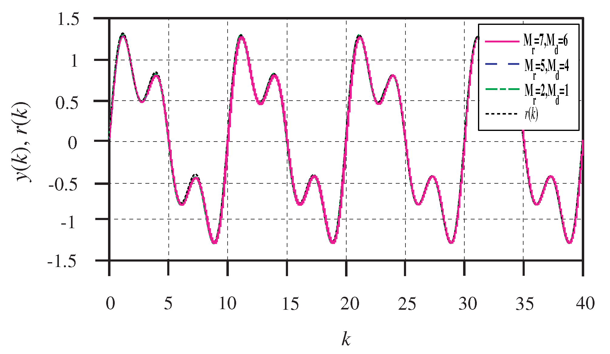
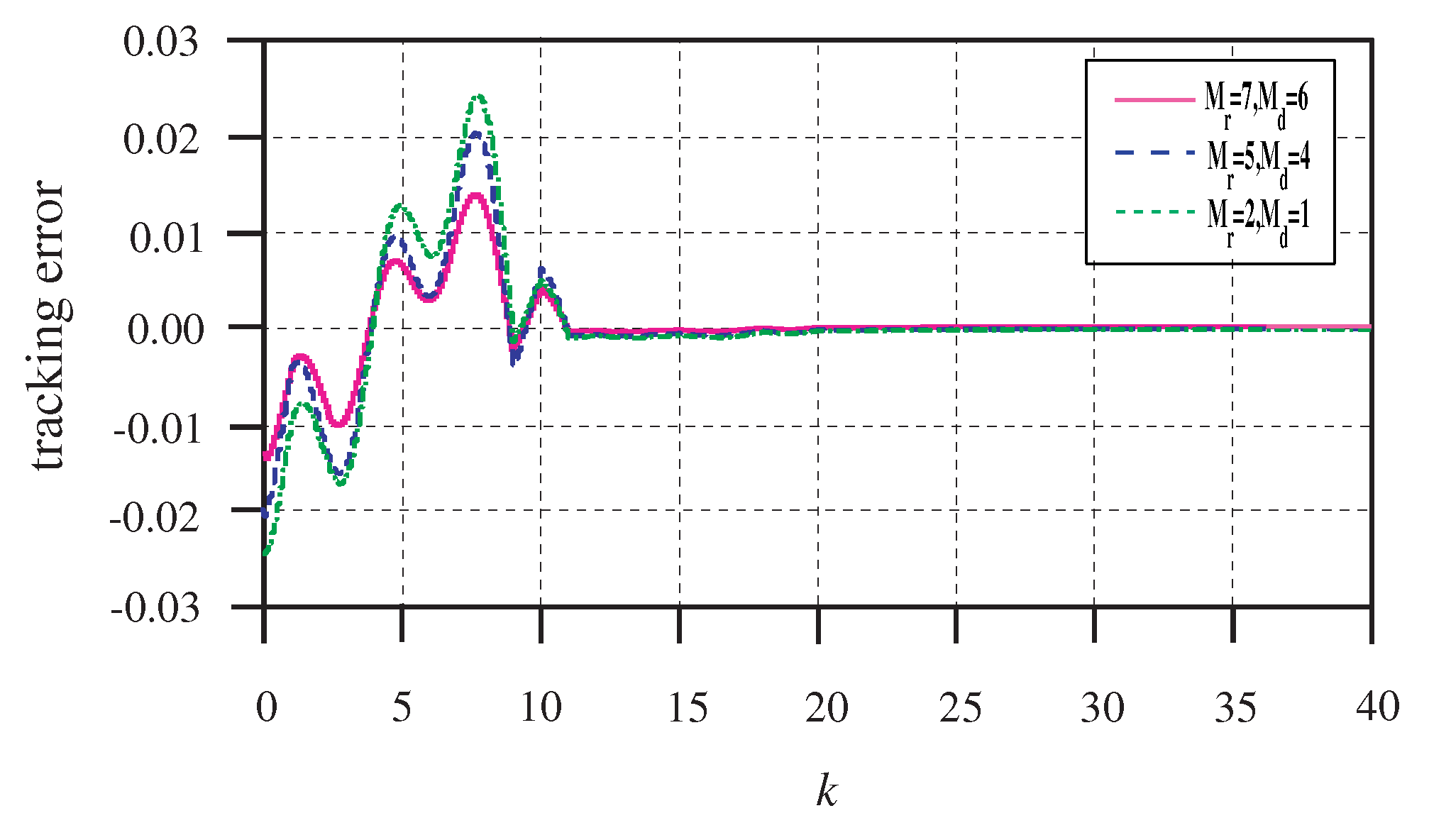
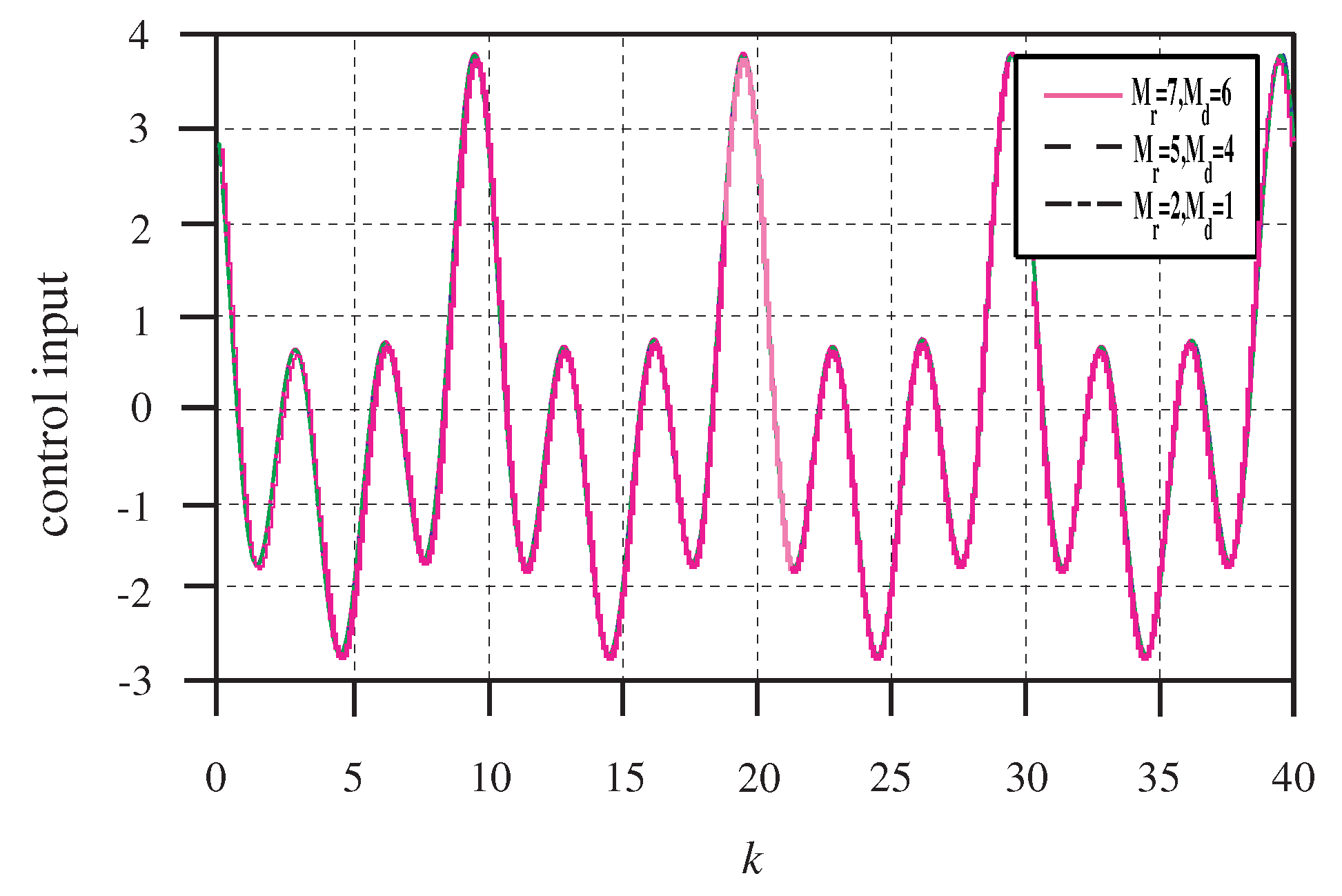
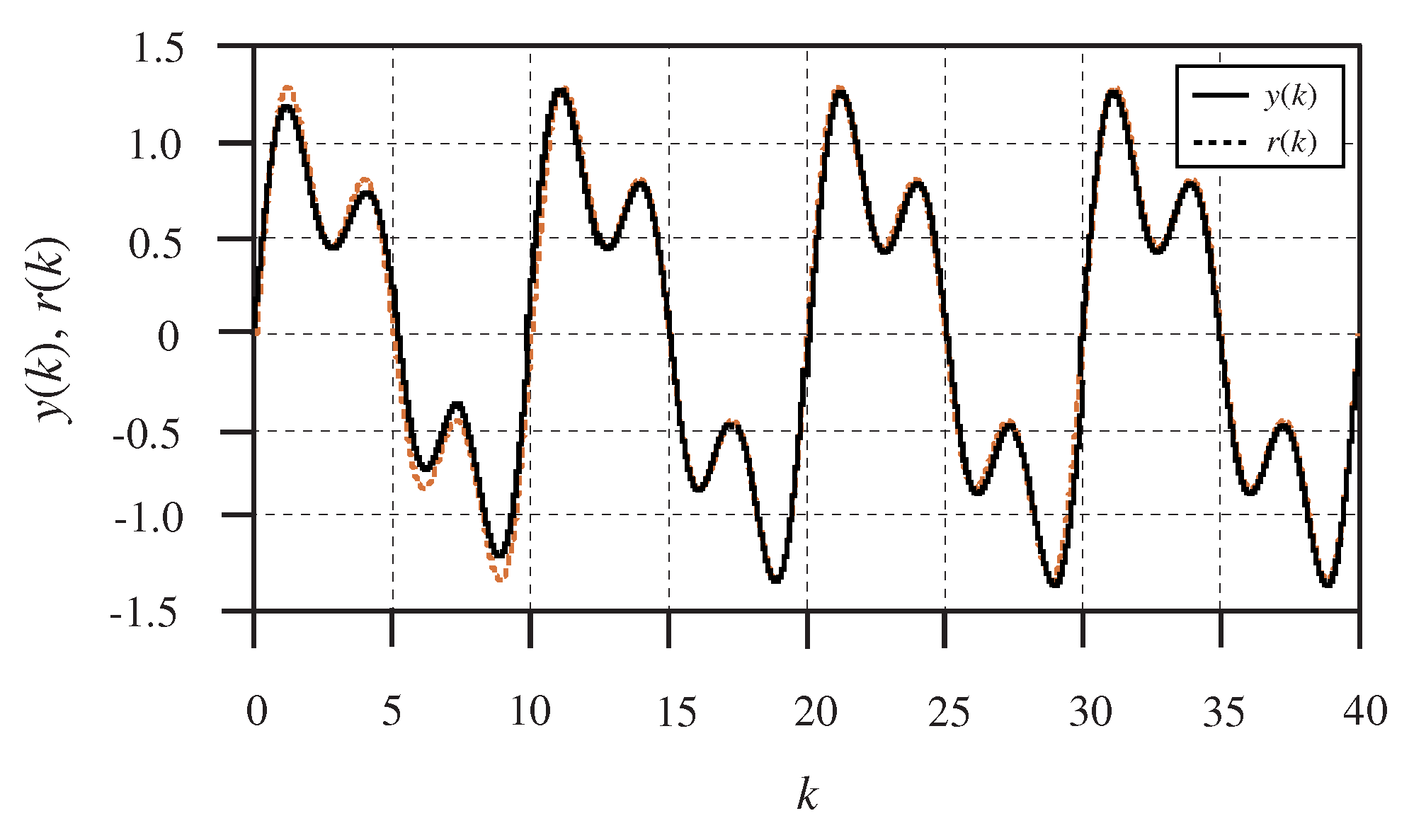
Figure 3 shows the reference signal $r\left(k\right)$ and the output $y\left(k\right)$ of the closed-loop system (1). The tracking errors and control inputs are depicted in Figure 4 and Figure 5, respectively. It can be seen from Figure 3 and Figure 4 that all of the outputs can track the reference signal accurately. Particularly, the repetitive control with preview compensator can effectively reduce the tracking error. In addition, the tracking error peak decrease is faster with an increase of the preview length.

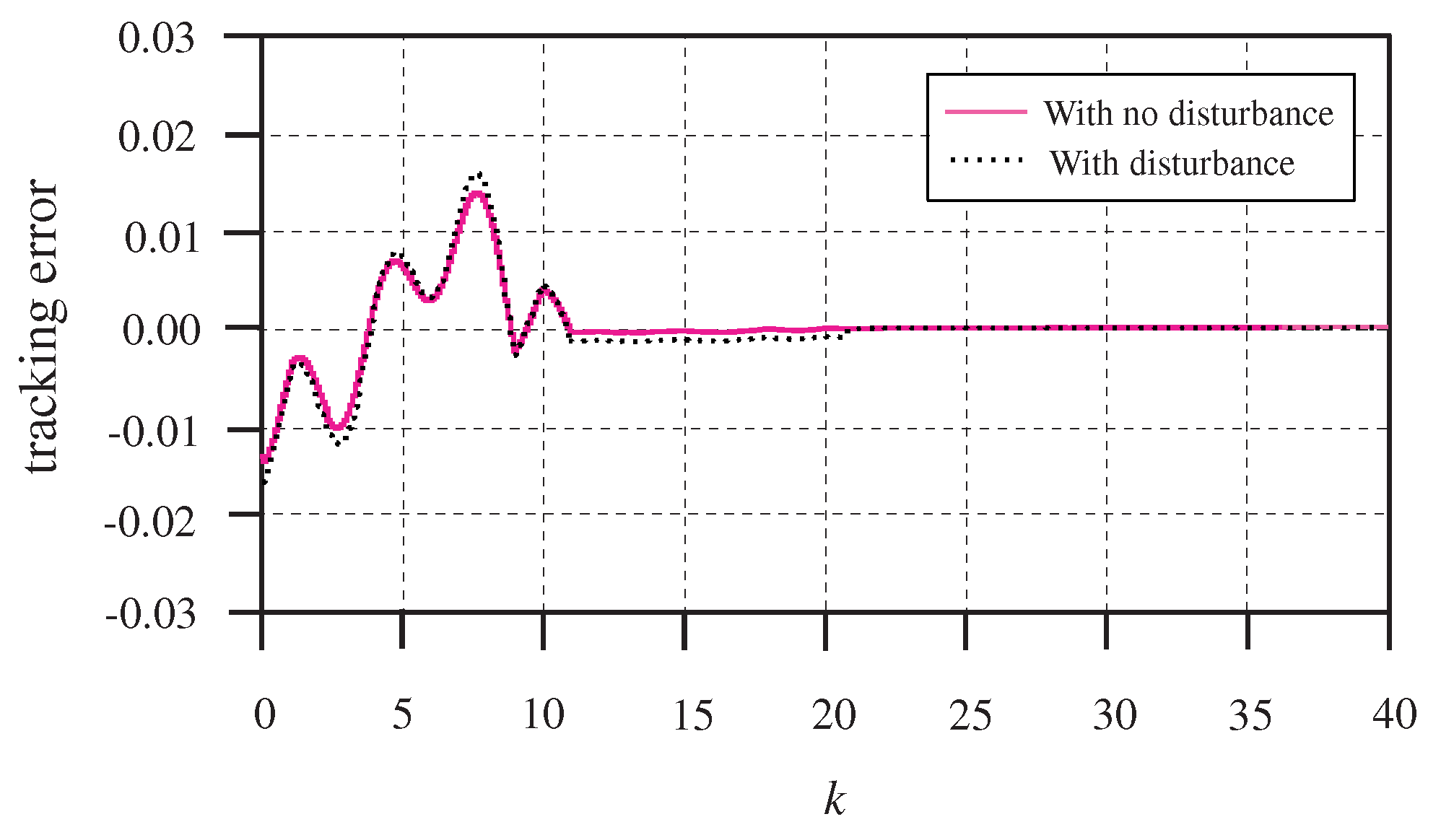
Note that a perfect estimation of the disturbance signal can hardly be available in practical applications. Next, the robustness of the proposed controller, with respect to the previewed disturbance signal, will be checked. To this end, in the case of $M_r=7,M_d=6$, we added an exogenous disturbance $\omega \left(k\right)=0.5cos\left(\frac{2\pi }{5}k\right)$ in the forward control input channel. Figure 6 illustrates that the output can track the reference signal effectively, even with the exogenous disturbance. The preview repetitive controller guarantees the robustness of the closed-loop system.

As pointed out in [2,4,5], the previewable reference and the disturbance signals have significantly impacted performance in the control system only for a certain time period, during which the reference signal exceeds the preview length, and the impact is very small. In the following, the limited performance with respect to the preview length will be inspected. To simplify this discussion, we set $M_d=0,$ and let the preview length of $M_r$ be $M_r\in \{1,2,7,8,9\}.$

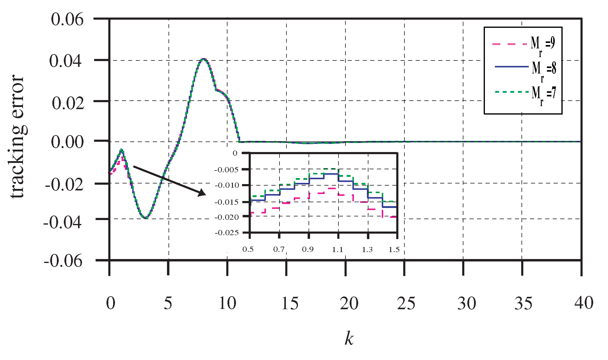
By solving the LMIs (36) in Theorem 3, the gain matrices are obtained in

Table 1. Gain matrices with different preview length of $M_r$.

${\mathit{M}}_{\mathit{r}}$	${\mathit{K}}_{\mathit{e}}$	${\mathit{K}}_{\mathit{y}}$	${\mathit{K}}_{\mathit{r}}$
1	[0.0563 −0.0045 −0.0019 −0.0009 −0.0009 −0.0013	−2.3632	[−0.0104 2.5237]
	−0.0023 −0.0007 0.0397 2.4240]
2	[−0.0451 −0.0073 −0.0014 −0.0004 −0.0008 −0.0008	−2.2864	[−0.0085 2.4135 0.0452]
	−0.0026 0.0006 0.0385 2.4005]
7	[0.0300 −0.0062 −0.0014 -0.0005 −0.0004 −0.0007	−2.2472	[−0.0035 2.3169 0.0380 −0.0002 −0.0015 −0.0011
	−0.0012 0.0003 0.0378 2.3170]		−0.0008 −0.0010]
8	[0.0302 −0.0062 −0.0016 −0.0005 −0.0004 −0.0007	−2.2472	[−0.0038 2.3175 0.0382 −0.0002 −0.0014 −0.0010
	−0.0012 0.0001 0.0379 2.3173]		−0.0006 −0.0007 −0.0022]
9	[0.0306 −0.0066 −0.0015 −0.0005 −0.0004 −0.0007	−2.2483	[−0.0040 2.3196 0.0378 −0.0001 −0.0013 −0.0009
	−0.0012 −0.0001 0.0379 2.3173]		−0.0006 −0.0007 −0.0018 −0.0081]

. The tracking error curves, corresponding with the preview length $M_r=7,8,9$, are shown in Figure 7. From Table 1 and Figure 7, we see that the gain matrices have little change when the preview length exceeds 7. The closed-loop control system achieves the best performance when $M_r=7$. It indicates that, when the preview length reaches a certain degree, there is almost no effect on the output response, which is consistent with Remark 6 and the conclusion of preview control theory [9,12,19].

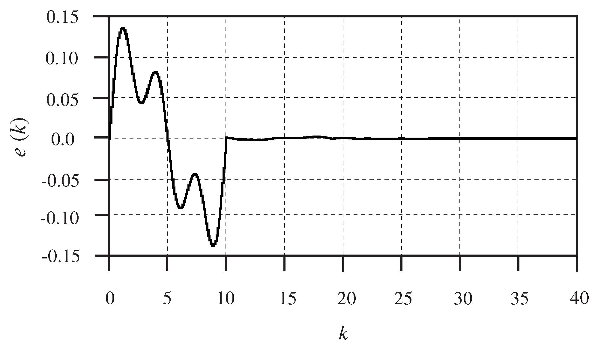
Finally, for comparison, we let $M_r=M_d=0$, to design a conventional guaranteed-cost repetitive-controller [34,35]. The best results are shown in Figure 8 and Figure 9. From the comparison, we can see that the preview repetitive controller provides better performance than the repetitive controller with no preview compensation.

6. Conclusions

This paper presented a design method of a guaranteed-cost preview repetitive controller for a class of polytopic uncertain discrete-time systems. Using the L-order forward difference operator, an augmented dynamic system was first constructed. Based on that, a guaranteed-cost static output feedback controller was then designed. By incorporating this controller into the original system, the guaranteed-cost preview repetitive controller was obtained. Simulation results verified the proposed method to be very effective. Our future work includes ILC and high-order ILC with preview compensation. Moreover, the case of continuous dynamics will also be included.

References

1. Katayama, T.; Ohki, T.; Inoue, T.; Kato, T. Design of an optimal controller for a discrete-time system subject to previewable demand. Int. J. Control 1985, 23, 667–699. [Google Scholar] [CrossRef]
2. Tsuchiya, T.; Tadashi, E.; Liao, T.b.F.C. Digital Preview and Predictive Control; Beijing Science and Technology Press: Beijing, China, 1994. [Google Scholar]
3. Liao, F.; Tsuchiya, T.; Egami, T.; Xin, Y. Unified approach to optimal preview servo systems and optimal preview for compensated systems. Chin. J. Autom. 1998, 10, 329–336. [Google Scholar]
4. Hamada, Y. Flight test results of disturbance attenuation using preview feedforward compensation. IFAC-PapersOnLine 2017, 50, 14188–14193. [Google Scholar] [CrossRef]
5. Li, L.; Liao, F.C. Robust preview control for a class of uncertain discrete-time systems with time-varying delay. ISA Trans. 2018, 73, 11–21. [Google Scholar] [CrossRef] [PubMed]
6. Zhen, Z.Y.; Jiang, S.Y.; Ma, K. Automatic carrier landing control for unmanned aerial vehicles based on preview control and particle filtering. Aerosp. Sci. Technol. 2018, 81, 99–107. [Google Scholar] [CrossRef]
7. Han, K.; Feng, J.; Li, Y.; Li, S. Reduced-order simultaneous state and fault estimator based fault tolerant preview control for discrete-time linear time-invariant systems. IET Control Theory Appl. 2018, 12, 1601–1610. [Google Scholar] [CrossRef]
8. Matthew, O.T.; Theeraphong, W. Optimal LQ feedforward tracking with preview: Practical design for rigid body motion control. Control Eng. Pract. 2014, 26, 41–50. [Google Scholar] [Green Version]
9. Robert, H.M.; Robert, R.B.; Bram, S. The information structure of feedforward/preview control using forecast data. IFAC Proc. 2014, 47, 176–181. [Google Scholar]
10. Salton, A.T.; Chen, Z.; Zheng, J.; Fu, M. Constrained optimal preview control of dual-stage actuators. IEEE/ASME Trans. Mech. 2016, 21, 1179–1184. [Google Scholar]
11. Strohm, J.N.; Lohmann, B. Optimal feedforward preview control by fir filters. IFAC-PapersOnLine 2017, 50, 5115–5120. [Google Scholar] [CrossRef]
12. Jadidi, M.G.; Hashemi, E. Optimal preview control of the nao biped robot using a ukf-based state observer. In Proceedings of the 2016 IEEE International Conference on Advanced Intelligent Mechatronics, Banff, AB, Canada, 12–15 July 2016. [Google Scholar]
13. Birla, N.; Swarup, A. Optimal preview control: A review. Optim. Control Appl. Meth. 2015, 36, 241–268. [Google Scholar] [CrossRef]
14. Takaba, K. Robust preview tracking control for polytopic uncertain systems. In Proceedings of the 37th IEEE Conference on Decision and Control, Tampa, FL, USA, 23–25 December 1998. [Google Scholar]
15. Liao, F.; Wan, J.L.; Yang, G.H. LMI-based reliable robust preview tracking control against actuator faults. In Proceedings of the American Control Conference, Arlington, VA, USA, 25–27 June 2001. [Google Scholar]
16. Wang, D.; Liao, F.; Tomizuka, M. Adaptive preview control for piecewise discrete-time systems using multiple models. Appl. Math. Model. 2016, 40, 9932–9946. [Google Scholar] [CrossRef]
17. Zhen, Z.Y. Research development in preview control theory and applications. Acta Autom. Sin. 2016, 42, 172–188. [Google Scholar]
18. Li, L.; Liao, F.C. Parameter-dependent preview control with robust tracking performance. IET Control Theory Appl. 2017, 11, 38–46. [Google Scholar] [CrossRef]
19. Liao, F.; Li, L. Robust preview control for uncertain discrete-time systems based on LMI. Optim. Control Appl. Method 2017. [Google Scholar] [CrossRef]
20. Inoue, T.; Nakano, M.; Iwai, S. High accuracy control of a proton synchrotron magnet power supply. In Proceedings of the 8th Internat Fedaration on Automatic Control, Kyoto, Japan, 24–28 August 1981; pp. 216–221. [Google Scholar]
21. Wang, Y.; Wang, R.; Xie, X.; Zhang, H. Observer-based H fuzzy control for modified repetitive control systems. Neurocomputing 2018, 286, 141–149. [Google Scholar] [CrossRef]
22. Hanson, R.D.; Tsao, T.C. Discrete-time repetitive control of LTI systems sampled at a periodic rate. IFAC Proc. 1996, 29, 1458–1463. [Google Scholar] [CrossRef]
23. She, J.H.; Pan, Y.; Nakano, M. Repetitive control system with variable structure controller. In Proceedings of the 6th International Workshop on Variable Structure Systems, Gold Coast, Australia, 7–9 December 2000. [Google Scholar]
24. Sun, M.; Wang, Y.; Wang, D. Variable-structure repetitive control: a discrete-time strategy. IEEE Trans. Ind. Electron. 2005, 52, 610–616. [Google Scholar] [CrossRef]
25. Fan, J.; Kobayashi, T. Discrete repetitive control via positive real compensation. Trans. Soc. Instrum. Control Eng. 2009, 33, 308–310. [Google Scholar] [CrossRef]
26. Yuan, S.G.; Wu, M.; Xu, B.G.; Liu, R.J. Design of discrete-time repetitive control system based on two-dimensionalmodel. Int. J. Autom. Comput. 2012, 9, 165–168. [Google Scholar] [CrossRef]
27. Zhou, L.; She, J.H.; Wu, M. Design of a design of a discrete-time output-feedback based repetitive-control system. Int. J. Autom. Comput. 2013, 10, 343–349. [Google Scholar] [CrossRef]
28. Wang, Z.H.; Yi, L.Z.; Lan, Y.H.; Chen, C.X. Design of observer-based discrete repetitive-control system based on 2D model. J. Cent. South Univ. 2014, 21, 4236–4243. [Google Scholar] [CrossRef]
29. Ahn, H.S.; Chen, Y.Q.; Moore, K.L. Iterative learning control: Brief survey and categorization. IEEE Trans. Syst. Man Cybern. C Appl. Rev. 2007, 37, 1099–1121. [Google Scholar] [CrossRef]
30. Mandra, S.; Galkowski, K.; Aschemann, H. Robust guaranteed cost ILC with dynamic feedforward and disturbance compensation for accurate PMSM position control. Control Eng. Pract. 2017, 65, 36–47. [Google Scholar] [CrossRef]
31. Mandra, S.; Galkowski, K.; Rogers, E.; Rauh, A.; Aschemann, H. Performance-enhanced robust iterative learning control with experimental application to pmsm position tracking. IEEE Trans. Control Syst. Technol. 2018, 1, 1–78. [Google Scholar] [CrossRef]
32. Park, J.H. Guaranteed cost stabilization of neutral differential systems with parametric uncertainty. Int. J. Comput. Appl. Math. 2003, 151, 371–382. [Google Scholar] [CrossRef]
33. Shi, P.; Boukas, K.K.; Shi, Y.; Agarwal, R.K. Optimal guaranteed cost control of uncertain discrete time-delay systems. Int. J. Comput. Appl. Math. 2004, 157, 435–451. [Google Scholar] [CrossRef]
34. Fu, C.; He, Y.; Wu, M.; Yuan, S. Guaranteed cost robust discrete repetitive control based on two-dimension model. In Proceedings of the 29th Chinese Control Conference, Beijing, China, 29–31 July 2010. [Google Scholar]
35. Lan, M.W.Y.H.; She, J.H.; He, Y. Design of nonfragile guaranteed-cost repetitive-control system based on two-dimensional model. Asian J. Control 2012, 14, 109–124. [Google Scholar]
36. Aleksander, H. Optimal linear preview control of active vehicle suspension. Veh. Syst. Dyn. 1992, 21, 167–195. [Google Scholar]
37. Marzbanrad, J.; Ahmadi, G.; Jha, R. Optimal preview active control of structures during earthquakes. Eng. Struct. 2004, 26, 1463–1471. [Google Scholar] [CrossRef]
38. Tomizuka, M.; Tsao, T.C.; Chew, K.K. Analysis and synthesis of discrete-time repetitive controllers. Trans. ASME J. Dyn. Syst. Meas. Control 1989, 111, 353–358. [Google Scholar] [CrossRef]
39. Boyd, S.; Ghaoui, L.; Feron, E. Linear Matrix Inequalities in System and Control Theory; SIAM Studies in Applied Mathematics: Philadelphia, PA, USA, 1994. [Google Scholar]
40. Nasiri, A.; Nguang, S.K.; Swain, A.; Almakhles, D.J. Robust output feedback controller design of discrete-time Takagi-Sugeno fuzzy systems: A nonmonotonic Lyapunov approach. IET Control Theory Appl. 2016, 10, 545–553. [Google Scholar] [CrossRef]
41. Chang, X.H.; Zhang, L.; Park, J.H. Robust static output feedback H control for uncertain fuzzy systems. Fuzzy Sets Syst. 2015, 273, 87–104. [Google Scholar] [CrossRef]
42. Kumar, E.V.; Raaja, G.S.; Jerome, J. Adaptive PSO for optimal LQR tracking control of 2 DoF laboratory helicopter. Appl. Soft Comput. 2016, 41, 77–90. [Google Scholar] [CrossRef]
43. Habib, M.; Khoucha, F.; Harrag, A. GA-based robust LQR controller for interleaved boost DC-DC converter improving fuel cell voltage regulation. Electr. Power Syst. Res. 2017, 152, 438–456. [Google Scholar] [CrossRef]
Figure 1. Basic discrete-time repetitive-control system.
Algorithms 12 00020 g001
Figure 2. Configuration of repetitive-control system with preview compensation.
Algorithms 12 00020 g002
Figure 3. The reference signal and the outputs of the closed-loop system with different preview length.
Algorithms 12 00020 g003
Figure 4. The tracking errors with different preview length.
Algorithms 12 00020 g004
Figure 5. The control inputs with different preview length.
Algorithms 12 00020 g005
Figure 6. The tracking errors with exogenous disturbance in the case of M r = 7 , M d = 6 .
Algorithms 12 00020 g006
Figure 7. The tracking errors with different preview length of M r .
Algorithms 12 00020 g007
Figure 8. The reference signal and the output of the system with no preview.
Algorithms 12 00020 g008
Figure 9. Tracking error with no preview.
Algorithms 12 00020 g009