An Opportunistic Network Routing Algorithm Based on Cosine Similarity of Data Packets between Nodes

Abstract

The mobility of nodes leads to dynamic changes in topology structure, which makes the traditional routing algorithms of a wireless network difficult to apply to the opportunistic network. In view of the problems existing in the process of information forwarding, this paper proposed a routing algorithm based on the cosine similarity of data packets between nodes (cosSim). The cosine distance, an algorithm for calculating the similarity between text data, is used to calculate the cosine similarity of data packets between nodes. The data packet set of nodes are expressed in the form of vectors, thereby facilitating the calculation of the similarity between the nodes. Through the definition of the upper and lower thresholds, the similarity between the nodes is filtered according to certain rules, and finally obtains a plurality of relatively reliable transmission paths. Simulation experiments show that compared with the traditional opportunistic network routing algorithm, such as the Spray and Wait (S&W) algorithm and Epidemic algorithm, the cosSim algorithm has a better transmission effect, which can not only improve the delivery ratio, but also reduce the network transmission delay and decline the routing overhead.

1. Introduction

The Opportunistic Network (OppNet) is a kind of ad-hoc network [1] that can complete information forwarding in the intermittently connected network environment, through the contact opportunity brought by the mutual movement between nodes. The OppNet is originated from the mobile ad-hoc network (MANET) [2] and the delay tolerant network (DTN) [3]. The communication of OppNet is different from the traditional wireless network. The most different point is that the nodes in the OppNet are not uniformly deployed, and they don’t need a completely connected transmission path between the sender and the receiver [4].

Because there is no complete end-to-end transmission path in the OppNet, the “storage-carrying-forwarding” routing mechanism is adopted for information transmission [5]. This method does not require the node to maintain the routing table to other nodes in the network. It is to cache information on a mobile node with storage capacity, and to find the right next hop nodes for information transmission with the help of the encounter opportunity brought by the movement of the node.

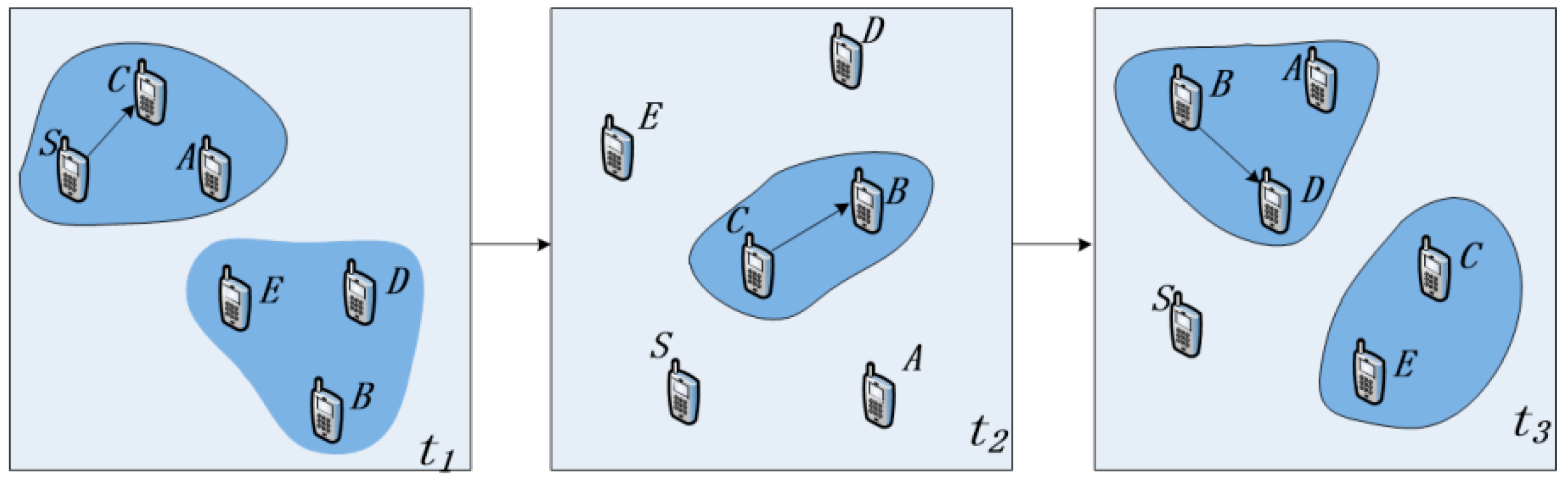
Figure 1 is a schematic diagram of the process of information transmission in an OppNet. Assume that the source node S needs to transmit information to the destination node D. Since node S and node D are not in the same connected domain at time t1, there is no complete communication link between them, so node S sends the message to the neighbor node C. Because node C does not have an appropriate next-hop for information transmission, it carries the message and waits for a suitable forwarding opportunity. With the opportunity of node mobility, node C and node B move to the same connected domain at time t2, and node C forwards the information to node B. Then, node B meets the destination node D at time t3, and forwards the message to node D to complete the information transmission.

In OppNet, there is no reliable communication link between source and destination nodes because the network connection is intermittent, the duration of network connection is short, and the network topology is constantly changing [6,7,8]. Due to the restrictions of various factors such as application characteristics, environment, and cost, OppNet can exactly meet the needs of certain specific applications [9]. Nowadays, the typical applications of the OppNet include the field data collection [10], the message communication in remote districts [11], the vehicle network [12], the ad hoc network under various environment [13], and so on.

Because the mobility of nodes in OppNet leads to the dynamic changing trend of the network topology, the traditional routing algorithms are difficult to apply to the OppNet. Therefore, how to select suitable neighbor nodes for information transmission in the topology has become one of the research hotspots in the field of the OppNet. At present, the research on the routing algorithm of the OppNet is mainly divided into two types, one kind is the proactive routing protocols [14], and the other kind is the reactive routing protocols [15]. However, due to the mobility of nodes in the OppNet and the intermittency of wireless connection, there is still the problems of low delivered ratio and unreasonable selection of next-hop nodes.

In the practical application scene, nodes in the network are usually people in a certain social relationship, and their mobility patterns and interactions are social [16]. In the OppNet with people as the carrier of the network terminal, human behavior characteristics and social attributes are different from other mobile network models [17], which play a decisive role in the design of routing algorithms. According to the small-world characteristics and agglomeration of human mobile behavior, the routing protocol based on the influence of nodes and community characteristics is proposed for message forwarding [18]. The regularity and social nature of human mobility can predict the future encounters of nodes to help select the best next hop nodes.

By analyzing the problems of some traditional routing algorithms of OppNet, combining the small-world effect and the relationship between the nodes, this paper considers how to choose the right neighbor node as the next hop from the perspective of social attributes between nodes. Practice has proved that the cosine similarity algorithm can accurately calculate the similarity between two texts [19]. In this paper, the cosSim routing algorithm based on cosine similarity is proposed to measure the strength of the social relations between nodes by calculating the cosine similarity between data packets of nodes, so as to select the next-hop nodes.

The paper is organized as follows: Section 2 describes the related work. Section 3 describes the proposed routing algorithm in detail. Experimentation and results are shown in Section 4 and, finally, in Section 5 some conclusions are drawn.

2. Related Work

Due to the dynamic change of the network topology caused by the node’s movement, the traditional routing protocols of wireless network are difficult to apply to the OppNet. Therefore, how to reasonably select the next hop to implement information forwarding effectively has become an important research direction of the OppNet [20].

The Epidemic algorithm [21] is based on the flooding strategy. The main idea is that nodes meet each other to exchange information which is missing from each other. The routing algorithm can enhance the delivered ratio of the network and reduce the transmission delay effectively, but it will generate a great deal of copies of messages in OppNet, which will easily lead to excessive routing overhead in the network.

Based on the traditional Epidemic algorithm, Zhang F et al. [22] proposed an Epidemic routing algorithm with adaptive capabilities. By observing the buffer status of the surrounding nodes, the algorithm adjusts the number of message copies injected by the node into the network in real time, which improves the performance of the Epidemic algorithm and effectively reduces the routing overhead.

A Spray and Wait algorithm is proposed in the literature [23]. The algorithm is divided into two stages: the Spray stage and the Wait stage. In the Spray stage, the sender forwards the message carried by itself to the network in a certain amount, and enters the Wait stage if it does not send the message to the receiver. During the Wait stage, all nodes carrying the message transmit the information to the receiving end through the Direct Delivery strategy. The main advantage of the Spray and Wait algorithm is that the routing overhead is significantly smaller than the Epidemic algorithm, and it has better scalability and can be well adapted to OppNets of various sizes.

The literature [24] proposed a routing algorithm based on the historical information (HBPR), which divides the network into different regional units and numbers them according to geographical locations. Each node uses GPS to record its own location information and count the most frequently visited areas. The source node transmits the message to a relay node that is geographically closer to the destination node, and continuously shortens the distance between the node carrying the message and the destination node, and achieves the effect of meeting the destination node and transmitting the message to it.

In the literature [25], the SRBet routing algorithm is proposed. First, the algorithm uses the temporal evolution graph model to accurately capture the dynamic topology structure of the OppNet. Based on the model, the algorithm introduces the social relationship metric for detecting the quality of human social relationship from contact history records. Utilizing this metric, the algorithm proposes social relationship based betweenness centrality metric to identify influential nodes to ensure messages forwarded by the nodes with stronger social relationship and higher likelihood of contacting other nodes.

The literature [26] proposed a protocol-social aware networking (SANE), it’s the first forwarding strategy that combines the advantages of both social-aware and stateless approaches in OppNet (also called pocket switched network, PSN) routing. Although cosine distance is used in the literature [26] and this article, there are obvious differences. The SANE protocol sets an interest space for each node in the network, and represents the interest space as an m-dimensional vector. And the cosine distance is used to calculate the similarity between nodes’ interest spaces. In this paper, we express the data packets of nodes by means of vectors, and the cosine distance is used to calculate the similarity between nodes’ data packets.

Fabbri F et al. [27] proposed a new sociable routing that selects a subset of optimal forwarders among all the nodes and relies on them for an efficient delivery. The important point is to assign a time-varying scalar parameter to each node in the network, which captures its social behavior in terms of frequency and types of encounters. Simulation results show that compared with other known protocols, the sociable routing achieves a good compromise in terms of delay performance and amount of generated traffic.

3. An Efficient Forwarding Strategy Based on Cosine Similarity between Nodes

For the problems in the process of forwarding information in the OppNet, this paper analyzes the relationships among nodes in the network and proposes an efficient forwarding strategy, cosSim, which is based on the cosine similarity of data packets between nodes. First, the algorithm calculates the cosine similarity of the data packets between nodes to define the relationship between nodes. Then according to the degree of similarity between the nodes to select the next hop for information forwarding.

3.1. Building the Opportunistic Network Topology

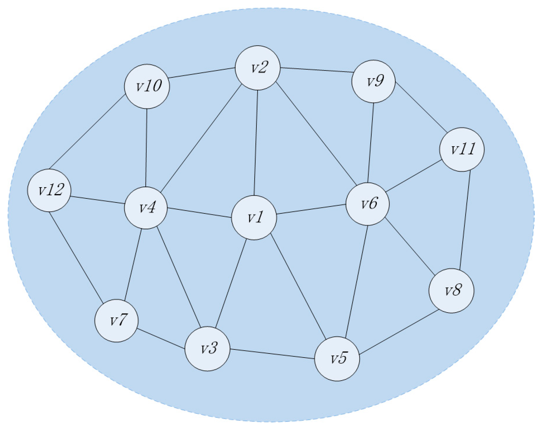
Assume that the selected sub-network topology is as shown in Figure 2. There are 12 nodes in total. The set of nodes is $V=\{V_1,V_2,\cdots ,V_{12}\}$. All nodes are relay nodes, all of which have the characteristics of mobility and the ability to carry and forward information. In current period, it is assumed that node $V_1$ needs to send information as the source node, and the speed of the message transmission between nodes is far greater than the speed of node movement. When the message is transmitted in sub-network, the sub-network topology will not change essentially.

In the OppNet, neighbor nodes of each node can transmit information, and each neighbor node may become the next-hop. Compared with the dynamically changing network topology, in the OppNet with people as the mobile carrier, the social relationships between nodes are relatively stable, it does not change with change of the network topology. The sociality of nodes are embodied in the data packets they carry. Therefore, it is necessary to select some nodes with relatively stable social relations among numerous neighbor nodes for information transmission.

This paper uses the cosine similarity to calculate the similarity of the data packets carried by nodes. The similarity of data packets between nodes is equal to the similarity between nodes, so as to define the strength of social relationships between nodes.

3.2. Node Definition and Similarity Calculation

Definition 1.

The data packet set $D_i=\{d_{i1},d_{i2},\cdots ,d_{ij}\}$ represents the j data packets carried by any node i. The data packets carried by the node i are expressed as a vector $C_i=(w_{i1},w_{i2},\cdots ,w_{ij})$, where $w_{ij}$ is the weight of the j-th data packet in the set $D_i$, that is the frequency of the data packet appearing in the node i, and the initial value is 1.

Definition 2.

The merge operation of the data packet sets of any two nodes a and b is denoted as $D^{\prime }=D_a\cup D_b$, and the respective data packet vectors are recalculated on the basis of the set $D^{\prime }$.

Assume that node a has a total of n data packets. Its set is

$$D_a=\{d_{a1},d_{a2},\cdots ,d_{ai},\cdots ,d_{an}\},1\le i\le n$$

(1)

The data packets of node a can be expressed as vector $C_a$:

$$C_a=(w_{a1},w_{a2},\cdots ,w_{ai},\cdots ,w_{an}),1\le i\le n$$

(2)

Assume that node b has a total of m data packets. Its set is

$$D_b=\{d_{b1},d_{b2},\cdots ,d_{bj},\cdots ,d_{bm}\},1\le j\le m$$

(3)

The data packets of node b can be expressed as vector $C_b$:

$$C_b=(w_{b1},w_{b2},\cdots ,w_{bj},\cdots ,w_{bm}),1\le j\le m$$

(4)

The merge operation of the data packet sets of node a and b is recorded as

$$D_{ab}=D_a\cup D_b=\{{d^{\prime }}_1,{d^{\prime }}_2,\cdots ,{d^{\prime }}_k,\cdots ,{d^{\prime }}_z\},1\le k\le z,\max (m,n)\le z\le (m+n)$$

(5)

The data packets vector of node a corresponds to the data packet set after merging is ${C^{\prime }}_a$:

$${C^{\prime }}_a=({w^{\prime }}_{a1},{w^{\prime }}_{a2},\cdots ,{w^{\prime }}_{ak},\cdots ,{w^{\prime }}_{az}),1\le k\le z$$

(6)

${w^{\prime }}_{ak}$ is calculated as follows:

$${w^{\prime }}_{ak}=\{\begin{array}{ll}{w}_{ai},& if{d^{\prime }}_k=d_{ai}\\ 0,& if{d^{\prime }}_k\ne d_{ai}\end{array}$$

(7)

The data packets vector of node b corresponds to the data packet set after merging is ${C^{\prime }}_b$:

$${C^{\prime }}_b=({w^{\prime }}_{b1},{w^{\prime }}_{b2},\cdots ,{w^{\prime }}_{bk},\cdots ,{w^{\prime }}_{bz}),1\le k\le z$$

(8)

${w^{\prime }}_{bk}$ is calculated as follows:

$${w^{\prime }}_{bk}=\{\begin{array}{ll}{w}_{bj},& if{d^{\prime }}_k=d_{bj}\\ 0,& if{d^{\prime }}_k\ne d_{bj}\end{array}$$

(9)

Definition 3.

The node similarity ${SIM}_{ab}$ indicates the degree of similarity between nodes a and b.

The cosine similarity between vector $Q$ and vector $D$ is as follows:

$$\cos (Q,D)=\frac{{\displaystyle \sum (Q{T}_i\times D{T}_i)}}{\sqrt{{\displaystyle \sum {(Q{T}_i)}^2}}\times \sqrt{{{\displaystyle \sum (D{T}_i)}}^2}}$$

(10)

Among them, $Q{T}_i$ and $D{T}_i$ represent the i-th element in vectors $Q$ and $D$ respectively.

By calculating the cosine of the angle between two vectors, the similarity between two vectors can be determined. Therefore, the similarity of two nodes, nodes a and b, can be calculated by combined data packet vectors ${C^{\prime }}_a$ and ${C^{\prime }}_b$, and its calculation formula is

$${SIM}_{ab}=\cos ({C^{\prime }}_a,{C^{\prime }}_b)=\frac{{\displaystyle \sum _1^z(w_{ak}\times w_{bk})}}{\sqrt{{\displaystyle \sum _1^z{(w_{ak})}^2}}\times \sqrt{{\displaystyle \sum _1^z{(w_{bk})}^2}}}$$

(11)

Definition 4.

Access control number K, which is used to control the number of the current node to access its neighbor nodes. When the current node has a large number of neighbor nodes, it may take a long time to attempt to access all the neighbor nodes, which is not conducive to the transmission of information in the network.

Therefore, when the number of neighbors of a node is larger than the access control number K, the neighbor nodes are sorted according to the transmission distance with the current node, and the first K neighbor nodes with closer transmission distance are preferentially accessed. The access control number K effectively reduces the computation time of the cosSim algorithm.

Definition 5.

The lower threshold of node similarity ($\alpha$), which is the screening criteria for candidate nodes in the next hop. When the degree of similarity between the current node and its neighbor node is greater than the lower threshold $\alpha$, the neighbor node is taken as a candidate node for the next hop.

If the similarity between the current node and all its neighbor nodes is less than that of the lower threshold $\alpha$, the neighbor node with the greatest similarity will be selected for information transmission.

Definition 6.

The upper threshold of node similarity ($\beta$). In the OppNet with people as the mobile carrier, if the similarity between the current node and one of its neighbor nodes is greater than the upper threshold $\beta$, it shows that the social properties of the two nodes are very similar. It is possible that their movement trajectories and the nodes they can reach are not much different. Therefore, it is not necessary to use this neighbor node as a candidate node for the next hop.

If the degree of similarity between the current node and all its neighbor nodes is greater than the upper threshold $\beta$, the neighbor node with the smallest similarity is selected for information transmission.

If the similarity between the current node and some neighbor nodes are less than the lower threshold $\alpha$, and the similarity with rest of the neighbor nodes is greater than the upper threshold $\beta$, Then, the neighbor node with the greatest similarity is selected as the next hop in all neighbor nodes whose similarity is less than the lower threshold $\alpha$. In all neighbor nodes whose similarity is greater than the upper threshold $\beta$, the neighbor node with the smallest similarity is selected as the next hop node for information transmission.

3.3. The Traversal Process of Node

Each node in the sub-network topology shown in Figure 2 maintains a buffer. The buffer stores the data packets that need to be forwarded by the node, and the each data packet has a globally unique identifier. Assume that the data packets of each node in the sub-network topology is shown in

Table 1. Data packet set and data packets vector of nodes.

Node	Data Packet Set	Data Packets Vector
$V_1$	{‘g’,‘h’,‘o’,‘p’}	(1,1,2,1)
$V_2$	{‘f’,‘g’,‘o’,‘p’}	(1,1,2,2)
$V_3$	{‘f’,‘j’,‘p’,‘t’}	(2,2,1,1)
$V_4$	{‘i’,‘o’,‘u’}	(1,1,1)
$V_5$	{‘f’,‘h’,‘i’}	(1,1,2)
$V_6$	{‘f’,‘j’,‘o’,‘p’}	(1,1,1,2)
$V_7$	{‘i’,‘l’,‘m’,‘s’}	(1,2,2,1)
$V_8$	{‘g’,‘f’,‘j’,‘p’}	(1,1,1,2)
$V_9$	{‘f’,‘j’,‘o’,‘p’}	(1,1,1,1)
$V_{10}$	{‘h’,‘p’,‘r’,‘s’,‘u’}	(2,3,2,1,1)
$V_{11}$	{‘f’,‘h’,‘o’,‘u’}	(1,2,1,3)
$V_{12}$	{‘g’,‘u’,‘s’,‘y’}	(2,1,1,1)

.

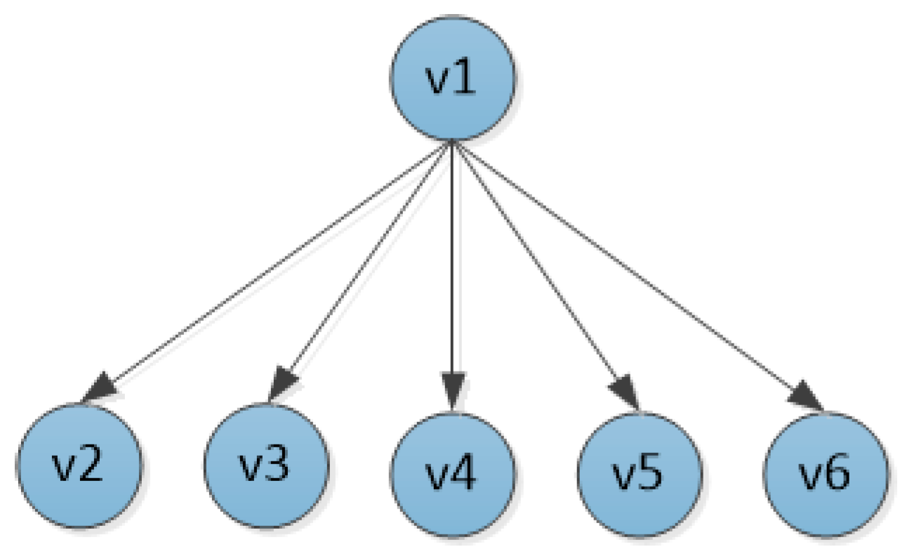
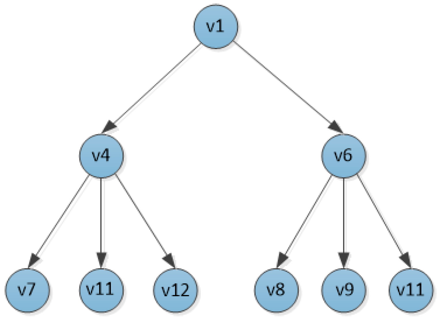
The node traversal process based on Figure 2 is as follows. First, initializes a directed tree T, which takes the node $V_1$ currently sending information as the root node. According to the transmission distance from node $V_1$, the first K neighbor nodes are inserted into the tree in turn as the children of node $V_1$, as shown in Figure 3.

The nodes $V_2$, $V_3$, $V_4$, $V_5$, $V_6$ are sequentially accessed to calculate their similarity to the current node $V_1$. The similarity calculation process of nodes $V_1$ and $V_2$ is as follows:

Merge the data packet sets of nodes $V_1$ and $V_2$:

$$D_{12}=D_1\cup D_2=\{f,g,h,o,p\}$$

(12)

Recalculate the data packet vectors of nodes $V_1$ and $V_2$:

$${C^{\prime }}_1=(0,1,1,2,1),{C^{\prime }}_2=(1,1,0,2,2)$$

(13)

Calculate the similarity between nodes $V_1$ and $V_2$:

$${SIM}_{12}=\cos ({C^{\prime }}_1,{C^{\prime }}_2)=\frac{0\times 1+1\times 1+1\times 0+2\times 2+1\times 2}{\sqrt{0^2+1^2+1^2+2^2+1^2}\times \sqrt{1^2+1^2+0^2+2^2+2^2}}=\frac{7}{\sqrt{7}\times \sqrt{10}}\approx 0.84$$

(14)

According to the above calculation process of the nodes $V_1$ and $V_2$, the similarities between the nodes $V_1$ and $V_3$, $V_4$, $V_5$, $V_6$ are calculated. The results are as follows: ${SIM}_{13}\approx 0.12$, ${SIM}_{14}\approx 0.44$, ${SIM}_{15}\approx 0.15$, ${SIM}_{16}\approx 0.57$.

Assume that both ${SIM}_{13}$ and ${SIM}_{15}$ are less than the lower threshold $\alpha$, ${SIM}_{12}$ is greater than the upper threshold $\beta$; ${SIM}_{14}$ and ${SIM}_{16}$ are located between the lower threshold and the upper threshold.

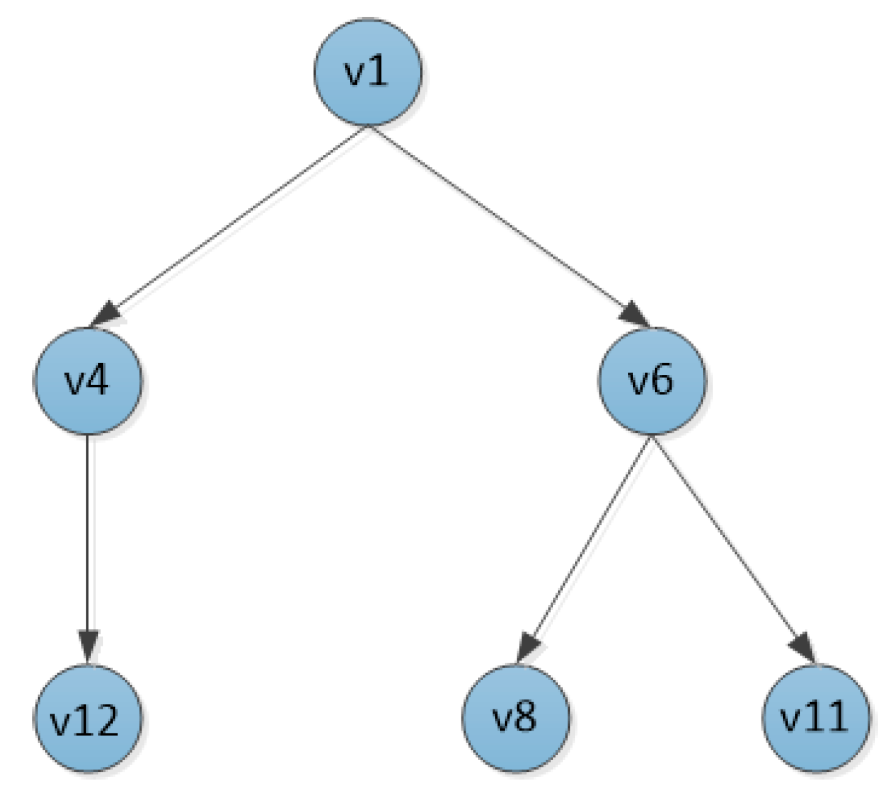
Therefore, the nodes $V_2$, $V_3$, and $V_5$ are deleted from the tree T, leaving nodes $V_4$ and $V_6$ as the next hop for node $V_1$. The neighbor nodes of nodes $V_4$ and $V_6$ are prioritized to insert the top K nodes into the tree T according to the transmission distance, as the children of the corresponding nodes.

At this point, the structure of the tree T is shown in Figure 4.

The neighbor nodes $V_7$, $V_{10}$ and $V_{12}$ of the node $V_4$, and the neighbor nodes $V_8$, $V_9$ and $V_{11}$ of the node $V_6$ are sequentially accessed to calculate the degree of similarity between the corresponding nodes. The results are as follows: ${SIM}_{47}\approx 0.18$, ${SIM}_{4,10}\approx 0.13$, ${SIM}_{4,12}\approx 0.22$, and ${SIM}_{68}\approx 0.86$, ${SIM}_{69}\approx 0.96$, ${SIM}_{6,11}\approx 0.20$.

Assume that ${SIM}_{47}$, ${SIM}_{4,10}$ and ${SIM}_{4,12}$ are all smaller than the lower threshold $\alpha$.

In this case, the node $V_{12}$ with the greatest similarity to the node $V_4$ is retained, and the remaining nodes $V_7$ and $V_{10}$ are deleted from the tree T.

Assume that ${SIM}_{68}$ and ${SIM}_{69}$ are both greater than the upper threshold $\beta$, and ${SIM}_{6,11}$ is smaller than the lower threshold $\alpha$.

Then node $V_{11}$ with the highest degree of similarity is retained in all nodes below the lower threshold. The node $V_8$ with the smallest similarity is retained in all nodes larger than the upper threshold, and the remaining node $V_9$ is deleted from the tree T.

At this point, the sub-network topology has been traversed and the final directed tree T is obtained, as shown in Figure 5, which is the transmission path graph of the sub-network.

3.4. Algorithm Design

According to the traversal process of nodes in the sub-network topological structure in the previous section, the routing algorithm based on cosine similarity of data packets between nodes is deduced. The execution process of the algorithm is as follows:

Step 1: Initialize a directed tree T. Each node maintains a set of data packets $D_i$ and a data packet vector $C_i$. The node S currently transmitting information is taken as the root node of the tree T.

Step 2: Create a set of neighbor nodes for the current node S, denoted as $U_s$.

If there is a parent node P of the current node in the tree T, create a set of neighbor nodes for the node P, denoted as $U_p$, and perform the following operation: $U_s=U_s-(U_s\cap U_p)$.

Step 3: Determine whether the number of nodes in the collection $U_s$ is greater than K. If the number of nodes in the set $U_s$ is greater than the access control number K, the nodes in the set are sorted from near to far according to the transmission distance from the current node, and the top K nodes are inserted into the tree T in turn as children of the current node S.

Step 4: Calculate the similarity between the current node s and each child node in turn.

First, merge the sets of data packets between node s and child node j, denoted as $D_{sj}=D_s\cup D_j$. According to the Equation (6), Equation (7) and the set of data packets after merging, the data packet vectors ${C^{\prime }}_s$ and ${C^{\prime }}_j$ of node s and node j are recalculated.

Then, based on the similarity calculation Equation (11), the similarity between nodes s and j is calculated, which is denoted as ${SIM}_{sj}$.

Step 5: Determine the similarity between the current node and each neighbor node.

All nodes with the value of similarity between the lower threshold $\alpha$ and the upper threshold $\beta$ are selected as the next hop, and the remaining nodes are deleted from the tree T.

If the similarity with all the neighbor nodes is less than the lower threshold, that is $\max ({SIM}_{sj})<\alpha$, the neighbor node with the greatest similarity is selected as the next hop, and the remaining child nodes are deleted from the tree T.

If $\min ({SIM}_{sj})>\beta$, the neighbor node with the smallest similarity is selected as the next hop, and the remaining child nodes are deleted from the tree T.

If $all({SIM}_{sj})\notin [\alpha ,\beta ]$. Then, among all the neighbor nodes whose similarity is less than the lower threshold $\alpha$, the neighbor node with the greatest similarity is selected as the next hop. And in all neighbor nodes whose similarity is greater than the upper threshold $\beta$, the neighbor node with the smallest similarity is selected as the next hop, and the remaining child nodes are deleted from the tree T.

Step 6: All children of the current node in the tree T are successively regarded as the current node, and steps 2, 3, 4, 5, 6 are repeated until the sub-network topology is accessed.

Step 7: According to the above process, a directed tree T can be finally obtained. In the light of the structure of the tree T, we can get one or more transmission paths, and the node that is currently sending information is forwarded on these paths through a replication forwarding strategy.

The cosSim routing algorithm is shown in Algorithm 1.

Algorithm 1. Opportunistic Network Routing Algorithm Based on Cosine Similarity of Data Packets between Nodes.

1. Input: A graph G(V, E), a source S, Dz: Data packet aggregation of node z, Cz: Data packet 2. Output: A or more paths 3. Init: InitTree(T), CurrentNode(i,s); /*set the node s as the current node i*/ 4. Set: T.setRootNode(i); Ui; /*A set of neighbor nodes of node i*/ 5. If(Node p=T.getParentNode(i)) then 6. Up; Ui=Ui-(Ui∩Up); 7. SortbyDistance(Us); Us.Delete(K); /*Sorting neighbor nodes in Ui according to the transmission distance, 8. and delete the neighbor nodes after K*/ 9. While(! Empty(Ui)) do 10. For(Neighbor j : Ui) do 11. Dij=Di$\cap$Dj; 12. C’i; C’j; /*Merge the data packets of the node i and node j, Recalculation of data packet 13. weight vectors of nodes*/ 14. SIMij=cos(C’i,C’j); /*calculate the cosine similarity between node i and node j*/ 15. End for; 16. If (all(SIMij)<$\alpha$ or all(SIMij)>$\beta$) then 17. selectNode(max(SIMij) or min(SIMij)); T.setChildNode(i,j); 18. Else If (onePart(SIMij)<$\alpha$ and theRest(SIMij)>$\beta$) then 19. selectNode(max(onePart(SIMij)) and min(theRest(SIMij))); T.setChildNode(i,j); 20. Else SelectNode(SIMij); T.setChildNode(i,j); /*select the similarity between r and R*/ 21. End if 22. For(ChildNode k : T.getChildNode(i)) do 23. setCurrentNode(i, k); continue; 24. end for; 25. Node p=T.getParentNode(i); Up; Ui= Ui- Up; Sort(Ui); Ui.Delete(K); 26. End while; 27. getPath(T); /*Gets the transmission paths based on the tree T*/ 28. Return T

4. Experiments and Results

In view of the cosSim routing algorithm proposed in the above section, this paper will use the OppNet simulation platform ONE to compare it with the traditional routing algorithms—the Spray and Wait (S&W) algorithm and the Epidemic algorithm. This paper will use the three indicators of delivery ratio, delivery delay, and routing overhead to compare the above three algorithms.

The simulation scenario settings are shown in

Table 2. Simulation environment.

Parameter	Value
Simulated time	20 h
Simulated area	5000 m × 4000 m
Velocity of a node	2~10 (m/s)
Rate of node transmission	300 kb/s
Maximum transmission range	10 m
Communication mode	Bluetooth
Node cache	10 MB
Size of data packet	20 kb~500 kb
Lifetime of data packet	2 h

.

The algorithm parameters as shown in

Table 3. Algorithm parameter setting.

Parameter	Value
$\alpha$	0.29
$\beta$	0.81
$K$	6.7

.

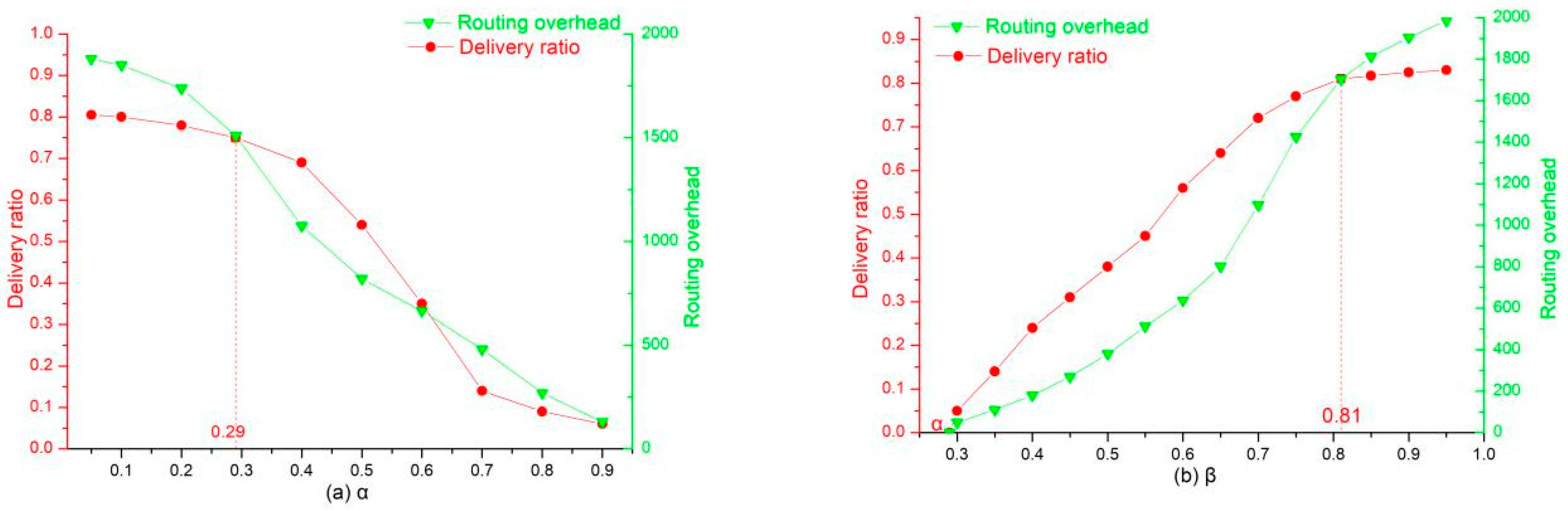
Through multiple simulation experiments, the upper and lower thresholds are selected based on the delivery ratio and routing overhead as reference values. The overall performance of the cosSim algorithm is relatively good when the lower threshold $\alpha$ = 0.29 and the upper threshold $\beta$ = 0.81. As shown in (a) of Figure 6, when the lower threshold $\alpha$ is equal to 0.29, the delivery ratio remains at a relatively high level, while the routing overhead of the network shows a significant decline when the lower threshold is greater than 0.29. As shown in (b) of Figure 6, when the upper threshold $\beta$ is greater than 0.81, the growth trend of the delivery ratio has been very slow, while the routing overhead is increasing, so the upper threshold is determined to be 0.81. When the access control number K is 6 or 7, the comparison times between nodes are not significantly increased, and the execution time of the algorithm can be effectively reduced. The following are analysis and comparison of the cosSim algorithm, S&W algorithm, and Epidemic algorithm in different situations.

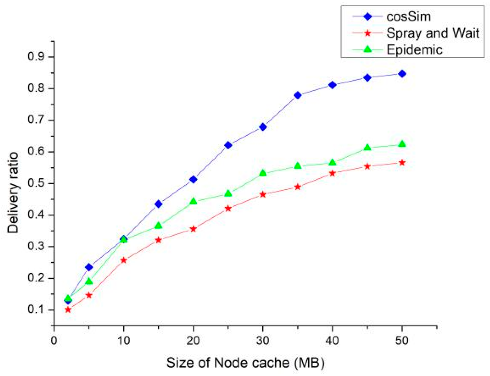
Figure 7 shows the delivery ratio of three routing algorithms with different node caches. According to Figure 7, the size of the node cache has the most significant effect on the delivery ratio of the cosSim algorithm. In the case where the node cache is small, the delivery ratio of the three routing algorithms is extremely low. With the increase of node caches, the delivery ratio of the three algorithms show different degrees of growth. The S&W and Epidemic algorithms show a slow growth trend. When the node cache is 50 MB, the delivery ratio of the S&W algorithm and the Epidemic algorithm are maintained at about 60% and 50%, respectively. The growth rate of delivery ratio of the cosSim algorithm is relatively fast. When the node cache is 25 MB, the delivery ratio of the cosSim algorithm has reached the highest level of the S&W algorithm and the Epidemic algorithm.

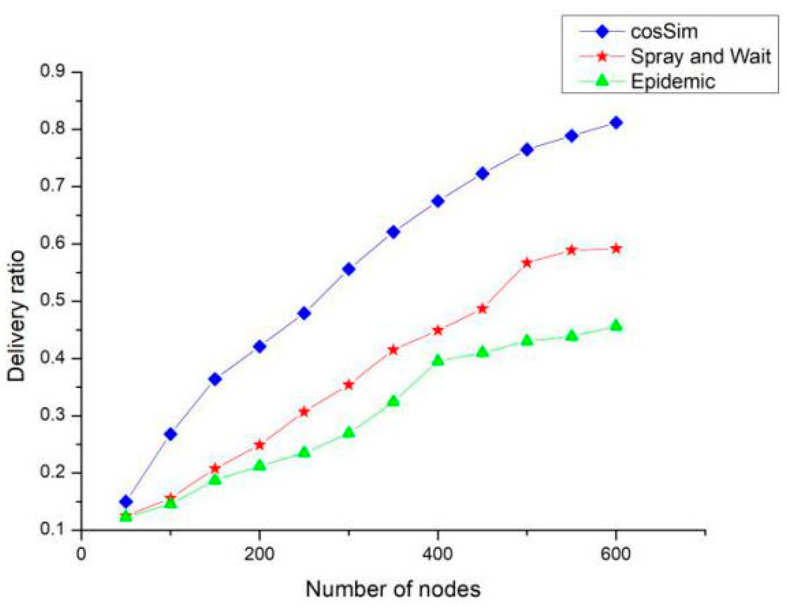
Figure 8 shows the effect of the number of nodes on the delivery ratio of the three algorithms, and the overall trend is similar to the node cache. The difference is that the delivery ratio of the Epidemic algorithm is always higher than the S&W algorithm when the node cache is getting larger. When the number of nodes is increasing, the delivery ratio of the S&W algorithm is always higher than the Epidemic algorithm. This shows that the Epidemic algorithm is more dependent on the node’s cache size, while the S&W algorithm is more dependent on the number of nodes in the network. When the number of nodes in the network reaches 600, the delivery ratio of the Epidemic algorithm and the S&W algorithm is 45% and 55% respectively, and the delivery ratio of the cosSim algorithm is as high as 80%.

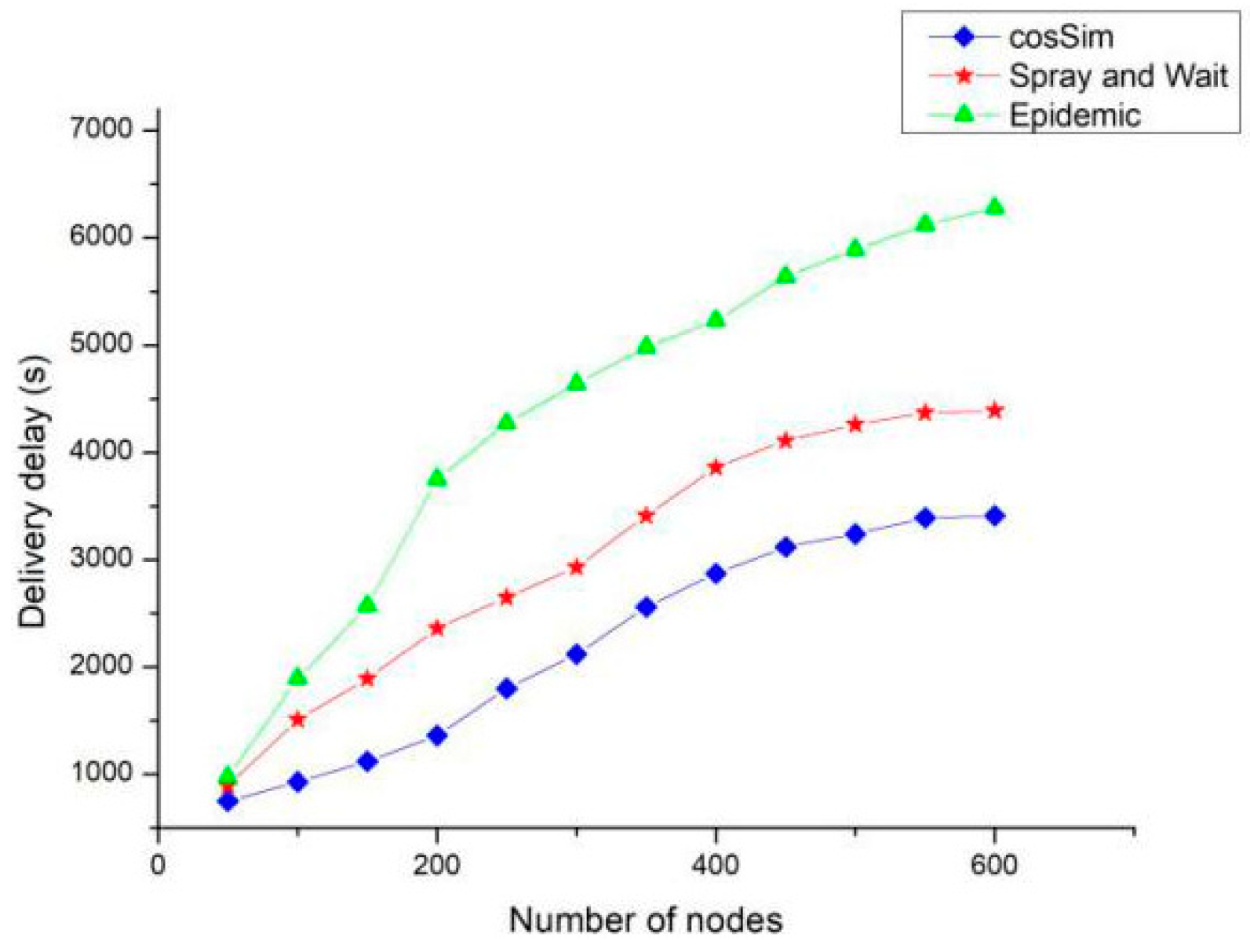
Figure 9 shows the performance of the three algorithms in terms of delivery delay under different number of nodes. The delivery delay of the cosSim algorithm is affected minimally by the change of the number of nodes, and the S&W algorithm and the Epidemic algorithm show the same growth trend. When the number of nodes is 600, the delivery delay of Epidemic algorithm and S&W algorithm is as high as 6500 and 5500 respectively. The delivery delay of the cosSim algorithm is slow. After the number of nodes is greater than 400, the delivery delay of the cosSim algorithm is maintained at around 3000, which is less than 2500 for the S&W algorithm and less than half for the Epidemic algorithm.

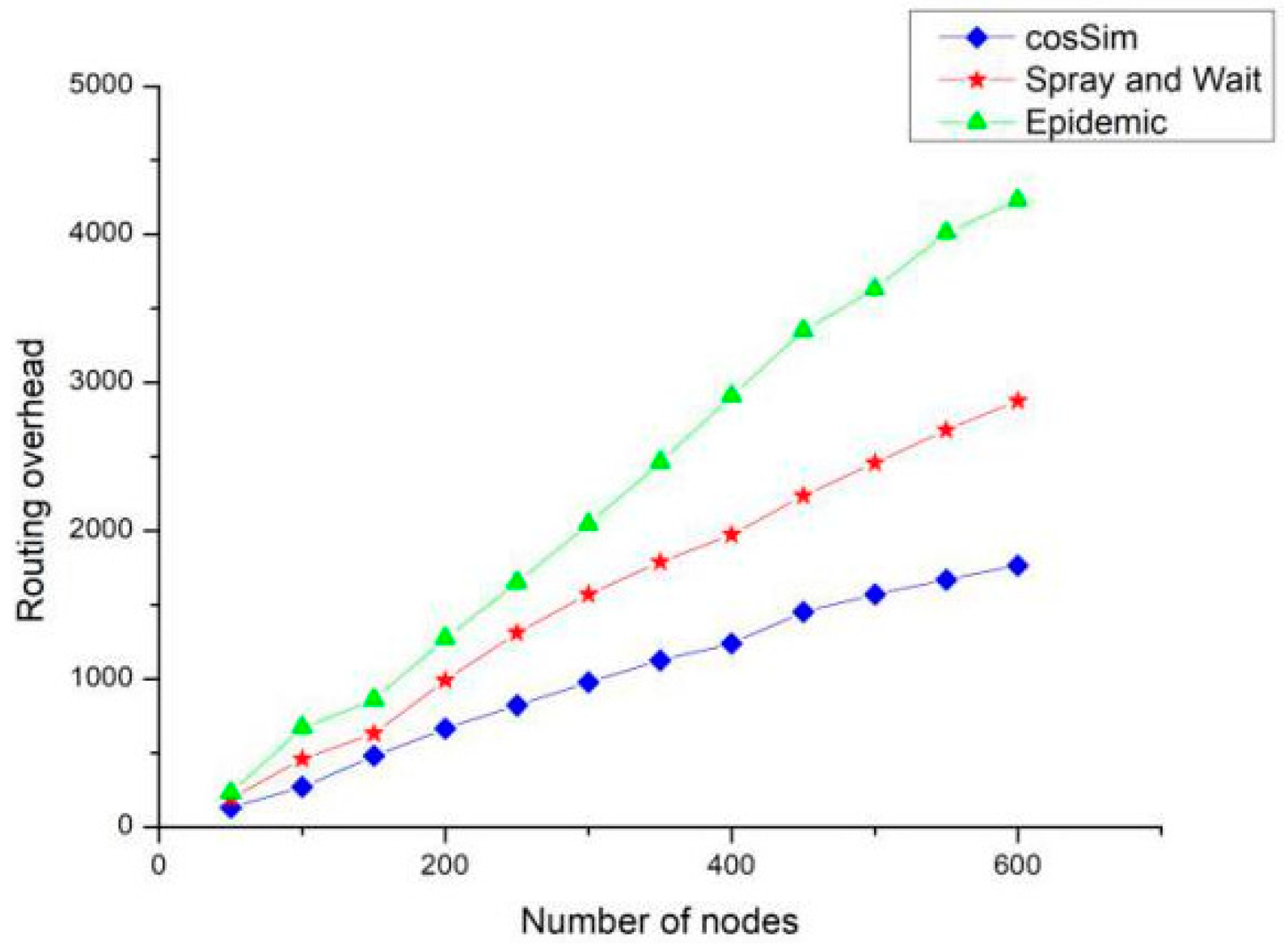
Figure 10 shows the effect of the number of nodes on the routing overhead of the three algorithms. As the number of nodes increases, the routing overhead of the three algorithms presents different growth trends. Among them, the Epidemic algorithm has the fastest growth rate of routing overhead, which is about twice the S&W algorithm and about three times that of the cosSim algorithm. When the number of nodes in the network is as high as 600, the routing overhead of the S&W algorithm is around 2500, that of the Epidemic algorithm is around 4500, and the routing overhead of the cosSim algorithm is the lowest around 1500. Because the Epidemic algorithm is based on the flooding strategy, it will generate a large number of copies in the network, which is likely to cause too much routing overhead.

The above simulation results show that compared with the traditional routing algorithms, S&W algorithm and Epidemic algorithm, the cosSim algorithm is more suitable for the data transmission of the OppNet, which can effectively improve the delivered ratio, and reduce the delivery delay and the routing overhead.

5. Conclusions

For the problems in the data forwarding process of the OppNet, this paper analyzes the relationship between the nodes and proposes a forwarding strategy based on the cosine similarity of data packets between nodes. By calculating the cosine similarity of data packets between nodes, the strength of social relationships between nodes is defined. By defining the upper threshold and the lower threshold, it is used to filter the neighbor nodes, and finally one or more valid transmission paths can be obtained in the sub-net.

Simulation experiments show that the cosSim algorithm performs much better than the traditional routing algorithms, the S&W algorithm and the Epidemic algorithm. The cosSim algorithm can improve the delivered ratio of the OppNet while effectively reducing the delivery delay and reducing the routing overhead. The cosSim algorithm provides a novel solution for the problems existing in the process of information transmission in OppNets.

In fact, the social properties of the nodes in the OppNet are very complex. The transmission process of messages between nodes is affected by various factors, such as the node’s mobile model and the community where the nodes are located. The comprehensive analysis of the above factors is the focus of the next step.