Abstract
The goal of object retrieval is to rank a set of images by their similarity compared with a query image. Nowadays, content-based image retrieval is a hot research topic, and color features play an important role in this procedure. However, it is important to establish a measure of image similarity in advance. The innovation point of this paper lies in the following. Firstly, the idea of the proximity space theory is utilized to retrieve the relevant images between the query image and images of database, and we use the color histogram of an image to obtain the Top-ranked colors, which can be regard as the object set. Secondly, the similarity is calculated based on an improved dominance granule structure similarity method. Thus, we propose a color-based image retrieval method by using proximity space theory. To detect the feasibility of this method, we conducted an experiment on COIL-20 image database and Corel-1000 database. Experimental results demonstrate the effectiveness of the proposed framework and its applications.
1. Introduction
Image retrieval is the procedure of retrieving relevant images from a big database of images, which usually occurs in one of two ways: text-based image retrieval or content-based image retrieval. Text-based image retrieval describes an image by using one or more keywords, but manual annotation has a huge cost burden. To address this defect, content-based image retrieval is introduced in [1]. Content-based image retrieval differs from traditional retrieval methods, as it uses visual contents such as key points, colors and textures to retrieve similar images from large scale image databases. Content-based image retrieval has been widely employed in several research fields, such as machine vision, artificial intelligence, signal processing, etc. Any content-based image retrieval system has two steps that can be explained as follows. The first step is feature extraction; the key point in this step is to find a method of feature extraction to precisely describe the content of image. Color features, which are the basic characteristic of the image content, are widely used in image retrieval [2,3,4,5]. For example, in [6], the color features was extracted in HSV color space by using color moment method. Gopal et.al. considered that only using grayscale information is imprecise in the image matching [7], because some images have same garyscale but have different color information, therefore they put color information into SURF descriptor making the precision better than only used SURF [8]. The second step is similarity measurement; in this step, the query image is selected, and the similarities between it and images of database are computed. In recent years, many different similarity computation methods have been proposed. Similarity is obtained by calculating the distance between two feature vectors, such as Euclidean, Manhattan and Chi square distance [9]. Chen et al. calculated similarities between the query image and images in database by comparing the coding residual [10]. Kang et al. proposed a similarity measure that is a sparse representation issue via matching the feature dictionaries between the query image and images of database [11]
With the rapid development of modern computer technology and soft computing theory, many modern algorithms and theories are applied to the image segmentation and image retrieval, which include fuzzy sets [12], rough set theory [13,14,15,16,17,18,19,20], near sets [21], mathematical morphology, neural network, etc. Computational Proximity (CP) [21] is a novel method to deal with image processing, which can identify nonempty sets of points that are either close to each other or far apart by comparing descriptions of pixels points or region in digital images or videos. Pták and Kropatsch [22] were the first to combine nearness in digital images with proximity spaces. In CP, pixel is an object, and the various features of pixel, such as grayscale, color, texture and geometry, are regarded as its attributes. For a point x, denotes the feature vector of x, then
Similarity between either points or regions in CP is defined in terms of the feature vectors that describe either the points or the regions. Feature vectors are expressed by introducing probe function. A probe maps a geometric object to a feature value that is a real number [21]. The similarity of a pair of nonempty sets is determined by the number of the same element. Put another way, nonempty sets are strongly near, provided sets have at least one point in common (introduced in [23]).
Example 1.
[21] Let be a nonempty sets of points in a picture, , where equals the intensity of the redness of A, equals the intensity of the greenness of A and equals the intensity of the blueness of A. Then,
From this, Region A resembles Region B, since both regions have equal blue intensity. Region A strongly resembles (is strongly near) Region C, since both regions have equal green and blue intensities. By contrast, the description of Region A is far from the descriptions of Region D or E, since Regions A and D or E do not have equal red or green or blue intensities.
From the above mentioned example, the description of an image is defined by a feature vector, which contains feature values that are real numbers (values are obtained by using probes, e.g., color brightness, and gradient orientation). It can be found that there are different feature values for different values. However, only several features play a distinguishing role for a object (set), so it is necessary to consider the order of features in matching description of another object. Specifically, for any nonempty set of points in an image, first we transform RGB color space into HSV (Hue, Saturation, Value) color space, and then 72 kinds of color features will be obtained by the color quantization. The HSV color space, which is closer to the human eye, is selected as the color feature representation of the image. Because human eye is limited to distinguish colors and if the range of each color component is too large, feature extraction will become very difficult. Thus, it is necessary to reduce the amount of computation and improve efficiency by quantifying the HSV color space component [24], and several dominant colors [25] are chosen, which can effectively match the image and reduce the computation complexity.
2. Proposed Method
This part presents the proposed method from two aspects, first is the transformation from RGB color space into HSV color space, and 72 kinds of color features will be obtained by the color quantization in HSV color space. Then, the similarity of images is identified by using proximity space theory. Second, we put forward an improved dominance granule structure formula as a similarity calculation method of proximity sets.
2.1. Feature Extraction
RGB color space and HSV color space are often used in digital image processing, and RGB color space is the basic color space that can be represented by a cube model. Red, green and blue are called the three primary colors and any point corresponds to a color in the RGB color model. HSV color space is established based on human visual perception characteristics and it can be represented by cone model. “Hue” means different color, “saturation” means the intensity of the color, whose value is in the unit interval [0,1], and “value” means the degree of shade of color. Circumferential color of the top of cone is pure color, and the top of the cone corresponds to , which contains three surfaces (R = 1, G = 1, and B = 1) in RGB color space. The conversion formula from RGB color space to HSV color space is given by:
where , and r, g, and b are the red, green and blue coordinates of a color, respectively, in RGB color space.
where and are the hue, saturation and value coordinates of a color, respectively, in HSV color space. Then, according to the property of the HSV color space, we can obtain 72 kinds of colors by the non-uniform quantization method, which can reduce the dimension of the color feature vectors and the amount of calculation. The quantization formula is described as follows:
Based on the above quantization method, the three-dimensional feature vector is mapped into a one-dimensional feature vector by using the equation: , where and are set to 3 because saturation and value are divided into three levels, respectively. Thus, the above equation can be rewritten as
According to the value range of h, s, and v, we can obtain the range of , and then we can get 72 kinds of color features.
2.2. Similarity Measure Based on Dominance Perceptual Information
Feature extraction and similarity measurement are two important steps in image retrieval. In this paper, color feature is selected as the retrieval feature, and we quantify color features into 72 numbers, . If an image X has T pixels, and there are Q pixels with the color feature c in an image, and . For example, , represents the probability that the color feature equals 0 in the image X, represents the probability that the color feature equals 1 in the image X, and represents the probability that the color feature equals 71 in the image X; then, we can obtain that , using which we can get a color histogram (see Figure 1) of a query image. The Top-m color features is obtained by descending order of , .
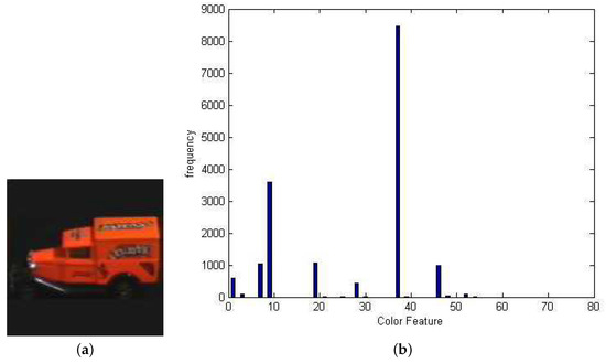
Figure 1.
(a) The query image; and (b) the color histogram of image (a).
In this paper, we take Top-m dominant color features in the HSV space to match images to improve the efficiency of retrieval; therefore, we use color features vector as the distinguishing description of image X. In addition, image similarity measurement is also important, such as Euclidean distance formula or cosine formula. However, if we use Euclidean distance formula or cosine formula to compute the similarity between the two images, in essence, it will lose significance. For example, the similarity between matrix and matrix is equal to 1 by cosine formula. Inspired by dominance rough set theory, we propose a novel dominance granule structure similarity method as similarity measurements, defined as follows:
Definition 1.
Let and , where X and Y represent the query image and the image of image database, respectively; and and represent the color attribute of X and Y, respectively. A is a set of all pre-order relationships on and . [26], and are the corresponding dominance granule structure, then the similarity between X and Y can be denoted by
because Equation (8) needs to calculate the global color feature similarity, the efficiency is reduced due to the large amount of calculation. Therefore, the Top-m color features of the image are selected for image matching, and Equation (8) is improved as follows:
where is the number of all the elements in set Φ, , and ,. The ordinal relation between objects in terms of the attribute or is denoted by ⪰, and or means that is at least as good as with respect to the attribute or .
Example 2.
To prove the feasibility of this method, we give an applied instance. Suppose , (description of query image I), where 7, 9 and 1 refer to the color features by quantization and . Let (description of ), (description of ), (description of ), etc represent the set of Top-3 color features of each image in image database, respectively. Thus, the similarity can be obtained by Equation (9) and results of the similarity are shown by Equation(10). , , ⋯, and represent images in the image database.
According to Equation (9), if , ,
| , | , |
, ,
As shown in Equation (10), we can see that the color feature’s order of is the same as the color feature’s order of I, so the similarity between and I is 1. Image strongly resembles (is strongly near) image I better than image , since the color feature’s order of is near to the color feature’s order of I. The image does not resemble image I, since both color features are different, so the similarity between and I is 0. Therefore, it makes it easier to match images if there exist more identical elements between color features. Simultaneously, it is also critical whether corresponding elements between features vector are equal, such as and image . The similarity measure proposed in this paper can improve the subjective and objective consistency of retrieval results.
2.3. Algorithm Flow Chart
As discussed above, the framework of our proposed method can be shown in Figure 2. The main procedures of the proposed framework are summarized as follows:
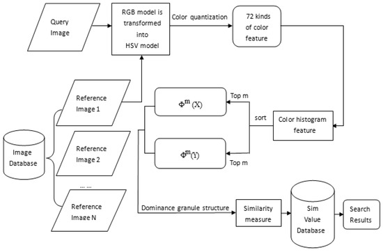
Figure 2.
The framework of the content-based image retrieval using proximity space theory.
Step 1: A query image in the RGB value (r,g,b) by nonlinear transformation converts to the HSV space value (h,s,v).
Step 2: We get 72 kinds of colors by the quantization.
Step 3: We obtain the color histogram of a query image and take the Top-m dominant color features forming the set of . We do the same with each image in the image database and get the set of .
Step 4: We use our proposed method for similarity measurements to calculate the similarity between the query image and the image of image database.
Experimental results with Top-20 images are shown in Figure 3 by using proposed similarity measurement, and the query image is the first one in each category.
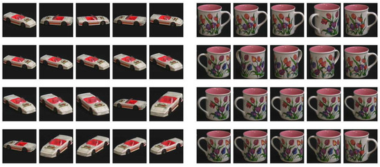
Figure 3.
The left image shows car category results, while the right image shows cup category results.
3. Experiment and Results
In this section, experimental results of the proposed method on COIL-20 [7] image database and Corel-1000 [10] database are presented. The COIL-20 database involves 1440 images, in which the images are separated into twenty categories (see Figure 4), and every category includes 72 images. The size of each image is . Table 1 shows the results of enhanced-surf method and our method, respectively, on COIL-20 database. is the number of relevant images retrieved, while is the total number of images retrieved. Thus, the precision and the recall of this retrieval system are given by Equation(11).
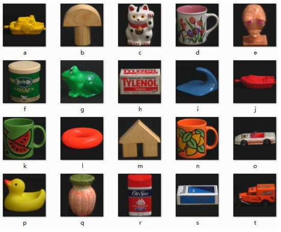
Figure 4.
Images selected from COIL-20 dataset.

Table 1.
Comparisons of precision and recall results among enhanced SURF method and our Proposed Method.
According to the results in Table 1b, we can get the average precision is 0.4818 and the average recall is 0.8387 by calculating the mean value of the third and fourth line, respectively. Compared with the enhanced SURF, these results demonstrate that the average precision and the average recall of our method increase by and , respectively.
The Corel-1000 database includes 1000 images from ten categories (African tribes, Beaches, Buildings, Buses, Dinosaurs, Elephants, Flowers, Horses, Mountains, and Foods) (see Figure 5).

Figure 5.
Ten classes on Corel-1000 dataset.
Each category contains 100 images with size of or . Each image in this database is taken to query. Table 2 shows the precision and recall results of our proposed method compared with CLD [27], Color Moment [28] and CSD [29].

Table 2.
Comparisons of precision and recall results among CLD, Color Moment, CSD and our Proposed Method.
Precision is computed from the Top-10 retrieved images and recall is calculated from the Top-100 retrieved images. CLD takes spatial information into account, but fails to find rotated or translated images that are similar to query images. Color moment has nine color components, with three low-order moments for each color channel, but low-order moments are less discriminating, so it is often used in combination with other features. CSD is mainly used for static image retrieval, and only considers whether the structure contains a certain color, and not about its frequency.
Table 2 shows that the average precision of our experimental results are , and higher than CLD, color moment and CSD, respectively; the average recall of our experimental results are , and higher than CLD, color moment and CSD, respectively; and our method retrieves buildings category images, the elephants category images and foods category images better than the other algorithms. For example, buildings images can be more precisely retrieved by using our method, and it can be seen that the average precision of our experimental results are , and higher than CLD, color moment and CSD, respectively; and the average recall of our experimental results are , and higher than CLD, color moment and CSD, respectively. The precision of dinosaurs category and flower category are highly retrieved in our proposed algorithm. Table 3 shows the precision rate of retrieving the Top-20 database images for each query image, while some retrieved images in the dinosaurs category, horses category and foods category are shown in Figure 6.

Table 3.
Precision rate for retrieving the Top 20 database images for each query image.
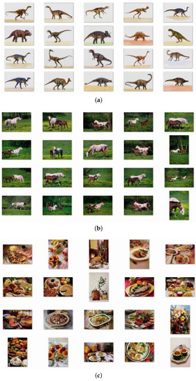
Figure 6.
Retrieved images for the Top 20: the dinosaurs category (a); (b) the horses category; and (c) the foods category. The query image is the first image in each class.
4. Conclusions
This paper provides a novel image similarity measurement method, which uses the improved dominance granule structure formula as a similarity calculation method of proximity sets. By simulating public datasets and comparing with other methods (CLD, Color Moment and CSD), it was found that the image retrieval based on this method produces a better retrieval result. The proposed method is meaningful to improve the retrieval accuracy, and provides a new attempt in the field of image retrieval.
Author Contributions
Conceptualization, J.W. and L.W.; Methodology, J.W.; Software, J.W.; Validation, J.W. and L.W.; Formal Analysis, J.W.; Writing-Original Draft Preparation, J.W.; Writing-Review & Editing, J.W., L.W., X.L. and Y.R.; Visualization, J.W.; Supervision, L.W., X.L., Y.R. and Y.Y.
Funding
This work was partially supported by Natural Science Foundations of China under Grant Nos. 61602321, 61773352, Aviation Science Foundation with No. 2017ZC54007, Science Fund Project of Liaoning Province Education Department with No. L201614, Natural Science Fund Project of Liaoning Province with No. 20170540694, the Fundamental Research Funds for the Central Universities (Nos. 3132018225, 3132018228) and the Doctor Startup Foundation of Shenyang Aerospace University13YB11.
Conflicts of Interest
The authors declare no conflict of interest.
References
- Amores, J.; Sebe, N.; Radeva, P.; Gevers, T.; Smeulders, A. Boosting Contextual Information in Content-Based Image Retrieval. In Proceedings of the 6th ACM SIGMM International Workshop on Multimedia Information Retrieval, New York, NY, USA, 15–16 October 2004; pp. 31–38. [Google Scholar]
- Zhang, Y.P.; Zhang, S.B.; Yan, Y.T. A Multi-view Fusion Method for Image Retrieval. In Proceedings of the International Congress on Image and Signal Processing, BioMedical Engineering and Information, Shanghai, China, 14–16 October 2017; pp. 379–383. [Google Scholar]
- Chen, Y.Y. The Image Retrieval Algorithm Based on Color Feature. In Proceedings of the IEEE International Conference on Software Engineering and Service Science, Beijing, China, 26–28 August 2016; pp. 647–650. [Google Scholar]
- Liang, C.W.; Chung, W.Y. Color Feature Extraction and Selection for Image Retrieval. In Proceedings of the IEEE International Conference on Advanced Materials for Science and Engineering, Tainan, Taiwan, 12–13 November 2016; pp. 589–592. [Google Scholar]
- Li, M.Z.; Jiang, L.H. An Improved Algorithm Based on Color Feature Extraction for Image Retrieval. In Proceedings of the International Conference on Intelligent Human-Machine Systems and Cybernetics, Hangzhou, China, 25–26 August 2016. [Google Scholar]
- Alhassan, A.K.; Alfaki, A.A. Color and Texture Fusion-Based Method for Content-Based Image Retrieval. In Proceedings of the International Conference on Communication, Control, Computing and Electronics, Khartoum, Sudan, 16–18 Janary 2017; pp. 1–6. [Google Scholar]
- Gopal, N.; Bhooshan, R.S. Content Based Image Reterieval using Enhanced SURF. In Proceedings of the Fifth National Conference on Computer Vision, Pattern Recognition, Image Processing and Graphics, Patna, India, 16–19 December 2015; pp. 1–4. [Google Scholar]
- Bay, H.; Ess, A.; Tuytelaars, T.; Gool, L.V. Speeded-Up Robust Features (SURF). Comput. Vis. Image Underst. 2008, 110, 346–359. [Google Scholar] [CrossRef]
- Kaur, M.; Sohi, N. A Novel Techinique for Content Based Image Retrieval Using Color, Texture and Edge Features. In Proceedings of the International Conference on Communication and Electronics System, Coimbatore, India, 21–22 October 2016; pp. 1–7. [Google Scholar]
- Chen, Q.S.; Ding, Y.Y.; Li, H.; Wang, X.; Wang, J.; Deng, X. A Novel Multi-Feature Fusion and Sparse Coding Based Framework for Image Retrieval. In Proceedings of the IEEE International Conference on Systems, Man, and Cybernetics Octobor, San Diego, CA, USA, 5–8 October 2014; pp. 2391–2396. [Google Scholar]
- Kang, L.W.; Hsu, C.Y.; Chen, H.W.; Lu, C.S.; Lin, C.Y. Feature-Based Sparse Representation for Image Similarity Assessment. IEEE Trans. Multimed. 2011, 13, 1019–1030. [Google Scholar] [CrossRef]
- Bakhshali, M.A. Segmentation and Enhancement of Brain MR Images using Fuzzy Clustering Based on Information Theory. Soft Comput. 2016, 21, 6633–6640. [Google Scholar] [CrossRef]
- Pawlak, Z. Rough sets, Proceedings of the 6th ACMSIGMM. Int. J. Comput. Inform. Sci. 1995, 256–341. [Google Scholar]
- Lim, K.Y.; Rajeswari, M. Segmenting Object with Ambiguous Boundary using Information Theoretic Rough Sets. Int. J. Electron. Commun. 2017, 77, 50–56. [Google Scholar] [CrossRef]
- Senthilkumaran, N.; Rajesh, R. Brain Image Segmentation using Granular Rough Sets. Int. J. Arts Sci. 2009, 3, 69–78. [Google Scholar]
- Roy, P.; Goswami, S.; Chakraborty, S.; Azar, A.T.; Dey, N. Image Segmentation using Rough Set Theory: A Review. Int. J. Rough Sets Data Analy. 2014, 1, 62–74. [Google Scholar] [CrossRef]
- Khodaskar, A.A.; Ladhake, S.A. Emphasis on Rough Set Theory for Image Retrieval. In Proceedings of the 6th ACM SIGMM International Conference on Computer Communication and Informatics, Coimbatore, India, 8–10 Janary 2015; pp. 1–6. [Google Scholar]
- Thilagavathy, C.; Rajesh, R. Rough Set Theory and its Applications Image Processing-A Short Review. In Proceedings of the 3rd World Conference on Applied Sciences, Engineering, Technology, Kathmandu, Nepal, 27–29 September 2014; pp. 27–29. [Google Scholar]
- Rocio, L.M.; Raul, S.Y.; Victor, A.R.; Alberto, P.R. Improving a Rough Set Theory-Based Segmentation Approach using Adaptable Threshold Selection and Perceptual Color Spaces. J. Electron. Imag. 2014, 23, 013024. [Google Scholar]
- Wasinphongwanit, P.; Phokharatkul, P. Image Retrieval using Contour Feature with Rough Set Method. In Proceedings of the International Conference on Computer, Mechatronics, Control and Electronic Engineering, Changchun, China, 24–26 August 2010; Volume 6, pp. 349–352. [Google Scholar]
- Peters, J.F. Computational Proximity—Excursions in the Topology of Digital Images; Springe: Berlin, Germany, 2016. [Google Scholar]
- Pták, P.; Kropatsch, W.G. Nearness in Digital Images and Proximity Spaces. In Proceedings of the 9th International Conference on Discrete Geometry, Nantes, France, 18–20 Apirl 2016; pp. 69–77. [Google Scholar]
- Peters, J.F. Visibility in Proximal Delaunay Meshes and Strongerly Near Wallman Proximity. Adv. Math. 2015, 4, 41–47. [Google Scholar]
- Ma, J. Content-Based Image Retrieval with HSV Color Space and Texture Features. In Proceedings of the International Conference on IEEE Web Information Systems and Mining, Shanghai, China, 7–8 November 2009; pp. 61–63. [Google Scholar]
- Yan, Y.; Ren, J.; Li, Y.; Windmill, J.; Ijomah, W. Fusion of Dominant Colour and Spatial Layout Features for Effective Image Retrieval of Coloured Logos and Trademarks. In Proceedings of the IEEE International Conference on Multimedia Big Data, Beijing, China, 20–22 April 2015; Volume 106, pp. 306–311. [Google Scholar]
- Schroder, B.S.W. Ordered Sets: An Introduction; Springer: Berlin, Germany, 2002. [Google Scholar]
- Messing, D.S.; Beek, P.V.; Errico, J.H. The MPEG-7 Colour Struture Descriptor: Image Description using Colour and Local Spatial Information. In Proceedings of the 2001 International Conference on Image Processing, Thessaloniki, Greece, 7–10 October 2001; pp. 670–673. [Google Scholar]
- Shih, J.L.; Chen, L.H. Colour Image Retrieval Based on Primitives of Colour Moments. IEE Proc. Vis. Image Signal Process. 2002, 149, 370–376. [Google Scholar]
- Kasutani, E.; Yamada, A. The MPEG-7 Color Layout Descriptor: A Compact Image Feature Description for High-Speed ImageNideo Segment Retrieval. In Proceedings of the International Conference on Image Processing, Thessaloniki, Greece, 7–10 October 2001; pp. 674–677. [Google Scholar]
© 2018 by the authors. Licensee MDPI, Basel, Switzerland. This article is an open access article distributed under the terms and conditions of the Creative Commons Attribution (CC BY) license (http://creativecommons.org/licenses/by/4.0/).