Short-Run Contexts and Imperfect Testing for Continuous Sampling Plans

Abstract

Continuous sampling plans are used to ensure a high level of quality for items produced in long-run contexts. The basic idea of these plans is to alternate between 100% inspection and a reduced rate of inspection frequency. Any inspected item that is found to be defective is replaced with a non-defective item. Because not all items are inspected, some defective items will escape to the customer. Analytical formulas have been developed that measure both the customer perceived quality and also the level of inspection effort. The analysis of continuous sampling plans does not apply to short-run contexts, where only a finite-size batch of items is to be produced. In this paper, a simulation algorithm is designed and implemented to analyze the customer perceived quality and the level of inspection effort for short-run contexts. A parameter representing the effectiveness of the test used during inspection is introduced to the analysis, and an analytical approximation is discussed. An application of the simulation algorithm that helped answer questions for the U.S. Navy is discussed.

1. Introduction

Harold F. Dodge developed the initial continuous sampling plan, referred to as CSP-1, as an effort to ensure a high level of quality for items without the burden of 100% inspection [1]. Under CSP-1, some defective items escape to customers because of a reduced inspection rate. Dodge’s work included analytical formulae for performance metrics that are easy to use. However, those formulas were designed for long-run production contexts, and therefore do not apply to finite-size batches of items. In addition, those formulas were designed under the assumption of perfect testing, and therefore do not apply to imperfect testing.

Dodge’s original long-run framework has been adapted to handle imperfect testing, and the appreciable effect of imperfect testing on the performance parameters of the sampling plan is well-understood [2]. The original long-run production framework was also adapted to account for short-run contexts [3,4]; however, the assumption of perfect testing was retained. In these references, analytical formulae were derived using a Markov chain modeling approach that was later generalized by a renewal-process approach so that more general continuous sampling plans could be analyzed [5]. Formulas for performance metrics of CSP plans resulting from the renewal-process approach were implemented in FORTRAN code [6]. It should be emphasized, however, that the formulas implemented in the FORTRAN code reflect an assumption of perfect testing.

This research develops a simulation algorithm for CSP-1 plans to provide a mechanism to understand the combined impact of short-run contexts and imperfect testing. To the best of our knowledge, this is the first attempt to combine these two important practicalities of CSP-1 sampling contexts. The simulation algorithm implements a test effectiveness parameter that enables recognition that defective items can escape the test procedure. A key output of the simulation is the probability distribution for the number of defective items that escape to customers. An application that answers sampling design questions for the United States Navy is presented and comparisons with analytical formula are discussed. User-friendly R code that implements the simulation algorithm is provided.

2. Background

2.1. Continuous Sampling Plans

Continuous sampling plans, introduced by Harold F. Dodge in 1943, are useful for establishing and improving the quality of production line items [1]. The process inspects items by alternating between 100% inspection, where all items are inspected, and reduced inspection, where only a fraction of the items are inspected. It then labels them as either defective or non-defective. When an inspected item is found to be defective, it is replaced with a non-defective item. Dodge’s plan estimates the Average Outgoing Quality (AOQ), which is the expected value of the defective rate for the process.

CSP-1 was the initial continuous sampling plan. However, modified versions, such as CSP-2 and CSP-3, were later published by Dodge and Torrey in 1951 [7]. The CSP-2 plan is a less-stringent modification of CSP-1, in that CSP-2 reverts back to 100% inspection only when two defective items occur spaced less than k units apart, where k is a specified value. The CSP-3 plan is identical to the CSP-2 plan, except when a defective item is found, the next four items require inspection. CSP-3 provides a method of inspection to avoid clusters of defective items. Readers are referred to [8] for a comparison and contrast of the different varieties of CSP plans.

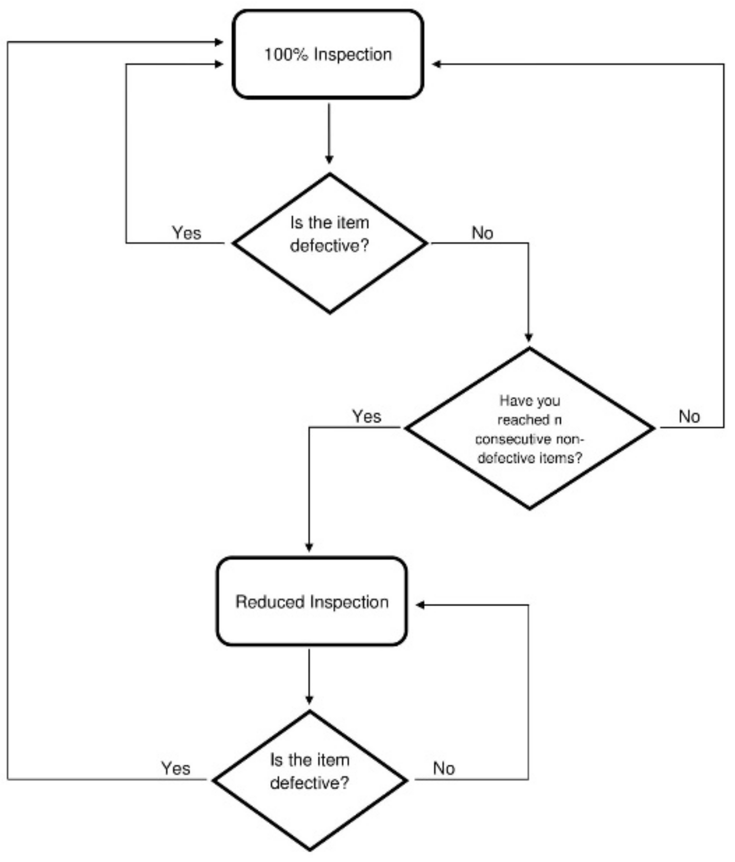
2.2. Operating Procedures for CSP-1

The CSP-1procedure is depicted in Figure 1. The process begins in 100% Inspection, in which every single item is sampled. The process breaks out of 100% Inspection when a specified number of consecutive non-defective items is reached, denoted as n. When the consecutive number of non-defective items is reached, the sampling procedure enters reduced inspection where the sampling process skips a specified number of items, skip. For example, if skip = 4 then you inspect every 5-th item. Sampling remains under reduced inspection until an item sampled is found to be defective. At that point, the process returns to 100% Inspection. Every time a sampled item is found to be defective, it is replaced with a non-defective item.

Figure 1. Operating Procedures for the initial continuous sampling plan (CSP-1).

The analytical formulas developed for CSP-1 assume infinite batch sizes and assume that the test is perfect. That is, defective items do not test as non-defective and non-defective items do not test as defective. The simulation algorithm we describe in the next section, and have implemented in the R code, relaxes both of these assumptions in order to extend the applicability of CSP-1 plans to short-run contexts that have imperfect testing. Navy applications often fall into this category, particularly since the units under examination can be very sophisticated electronic equipment that are difficult to exhaustively test.

3. Simulation Algorithm

The R function in Appendix A encodes the logic shown by the flowchart in Figure 2. The inputs to the R function are described in Section 3.1, and the outputs are described in Section 3.2.

Figure 2. Coding Flowchart. AOQ = Average Outgoing Quality; APS = Average Percent Sampled.

3.1. Inputs

Table 1 gives a description of the input variables. In Table 1, N represents the total number of items to be produced and delivered to the customer as a batch. F is the expected number of failures among the N items. In practice, a range of values for F can be considered to understand the influence it might have on AOQ. The required run length under 100% Inspection is denoted by n. The skip parameter represents the number of items skipped over while on reduced inspection. The parameter θ represents the probability a defective item is found to be defective by the test. We do not need to consider the case of a non-defective item testing as defective, because even if this were to happen the item would be replaced with another non-defective item.

Table 1. Input variables.

Variable	Description
N	Batch size
F	Failures in the batch
n	Required run under 100% inspection
skip	Items to skip over in reduced inspection
θ	Test effectiveness parameter

3.2. Outputs

Table 2 gives a description of the key output variables. For a given set of inputs, the algorithm runs 10,000 simulations of CSP-1 and outputs the AOQ and Average Percent Sampled (APS) values. AOQ is computed as the average (across the simulations) of the percentage of items in the batch that escape to the customer as defective, and the APS is computed as the average (across the simulations) number of items in the batch that are sampled. The algorithm can be used to tabulate AOQ as a function of F by running it with multiple choices for F. This will create multiple AOQ values, and the maximum of these values is defined as the Average Outgoing Quality Limit (AOQL).

Table 2. Output variables.

Variable	Description
AOQ	Average Outgoing Quality
APS	Average Percent Sampled

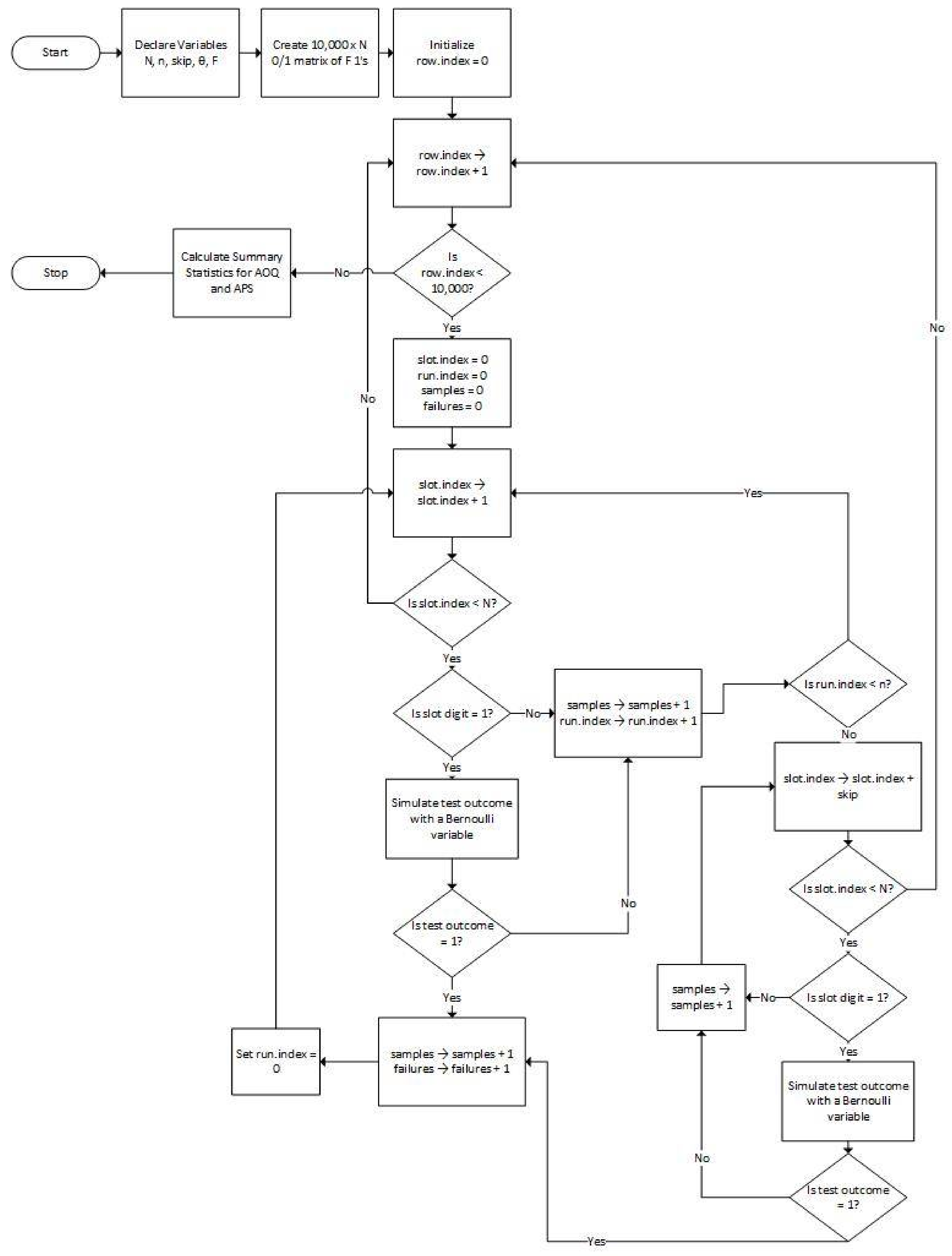
3.3. Algorithm Design

Figure 2 shows a flowchart that guided the design of the simulation algorithm. The essential idea of the design is to populate a matrix of 10,000 rows and N columns with 0 s and 1 s subject to the constraint that each row has F 1 s randomly slotted into the columns. The rows of the matrix are processed independently as batch replicates.

For each row, CSP-1 is simulated according to Figure 1. However, when a failed item is encountered, as indicated by reading a 1 from the row-column position, a Bernoulli (θ) random variable is simulated and the failure is only marked as detected if the Bernoulli outcome is also a 1. After each row of the matrix is processed, the total number of items sampled and the total number of failures in each batch are available for summary analyses.

The execution time of the simulation algorithm will depend primarily on the value of N. However, for our own use of the algorithm with batch sizes of 3200, the algorithm completed the calculations in less than a minute when executed on a typical Windows laptop computer.

4. Navy Applications

4.1. Background

The motivation for this research stemmed from a question the U.S. Navy wanted to answer. The U.S. Navy chose CSP-1 because it would allow them to be more efficient with time and money while still maintaining quality. Two particular CSP-1 plans were proposed and they sought advice on which was preferable. Both plans have N = 3200, F = 64, and skip = 4. However, the first plan, Plan 1, used n = 100, while the second, Plan 2, used n = 30.

4.2. Perfect Testing

For Plan 1, in which n = 100, the AOQ after CSP-1 is 0.66% and the APS is equal to 67.38%. For Plan 2, in which n = 30, the AOQ is equal 1.36% and the average percent sampled is equal to 32.18%. While the second CSP-1 plan sampled half as many items, the AOQ was twice as high. The Navy’s original question did not involve the implementation of the test effectiveness parameter; therefore, the testing procedure is assumed to be perfect in these two plans.

Figure 3 below illustrates the AOQ versus Initial Defective Rate and the APS versus Initial Defective Quality for both plans while varying the number of failures F from 0 to 320, where the Initial Defective Rate (IDR) is defined as F/N. We can see in Figure 3 that there is a mound shape to the AOQ graph, and the maximum AOQ is defined as the Average Outgoing Quality Limit (AOQL).

Figure 3. AOQ and APS for Navy sampling plans with perfect testing (top row is Plan 1 and bottom row is Plan 2). The top-left shows AOQ versus Initial Defective Rate for Plan 1 with perfect testing; the top-right shows APS versus Initial Defective Rate for Plan 1 with perfect testing; the bottom-left shows AOQ versus Initial Defective for Plan 2 with perfect testing; the bottom-right shows APS versus Initial Defective Rate for Plan 2 with perfect testing.

4.3. Imperfect Testing

This next example uses the same input values as the Perfect Testing example; however, the testing is imperfect with θ = 0.8, meaning that defective items are correctly identified 80% of the time.

For Plan 1, the AOQ after CSP-1 is 1.07% and the APS is equal to 58.15%. In Plan 2, the AOQ is 1.52% and the APS is 29.69%. In comparison to the perfect testing example, the AOQ is higher and the APS is lower. AOQ increases because defective items can escape the test procedure and end up in the batch that is delivered to the customers. APS decreases because some defective items are counted as non-defective, making it easier to switch to reduced inspection and therefore inspect less items.

Figure 4 below illustrates the AOQ versus Initial Defective Rate and the APS versus Initial Defective Rate for both plans while varying the number of failures F from 0 to 320. In this case, there is no mound shape and that is a consequence of imperfect testing. If θ ≥ 0.82, the mound shape returns. With imperfect testing, AOQ starts at 0 and increases to 1 − θ, with no guarantee that there is going to be a mound shape. The upper limit on AOQ of 1 − θ can be explained by considering what happens when the initial defect rate is large. In that case, it becomes increasingly difficult to move from 100% Inspection to reduced inspection, and under 100% Inspection the fraction of failed items that go undetected will be equal to the probability that the test fails to detect them, namely 1 − θ.

Figure 4. AOQ and APS for Navy sampling plans with imperfect testing (top row is Plan 1 and bottom row is Plan 2). The top-left shows AOQ versus Initial Defective Rate for Plan 1 with imperfect testing; the top-right shows APS versus Initial Defective Rate for Plan 1 with imperfect testing; the bottom-left shows AOQ versus Initial Defective Rate for Plan 2 with imperfect testing; the bottom-right shows APS versus Initial Defective Rate for Plan 2 with imperfect testing.

5. Analytical Comparisons

5.1. Calibration

Dodge developed mathematical expressions for AOQ and APS under his assumed context of infinite items being produced and perfect testing [1,9]. Let f denote the fraction of items inspected under Reduced Inspection.

$$f=\frac{1}{skip+1}$$

Dodge’s formulas derived

$$AOQ=p\left(1-APS\right)$$

$$APS=\frac{u+f v}{u+v}$$

where

$$u=\frac{1-q^n}{p q^n}$$

$$v=\frac{1}{f p}$$

$$p=probability of a defect$$

$$q=1-p$$

The formulas for AOQ and APS hold under perfect testing and when N = ∞. In order to apply them for a short-run context with perfect testing, we assign p as

$$p=\frac{F}{N}.$$

Note that this definition of p is the initial probability of defect, which is not constant throughout sampling procedure in short-run contexts. Consequently, the formula above for AOQ and APS will be approximations.

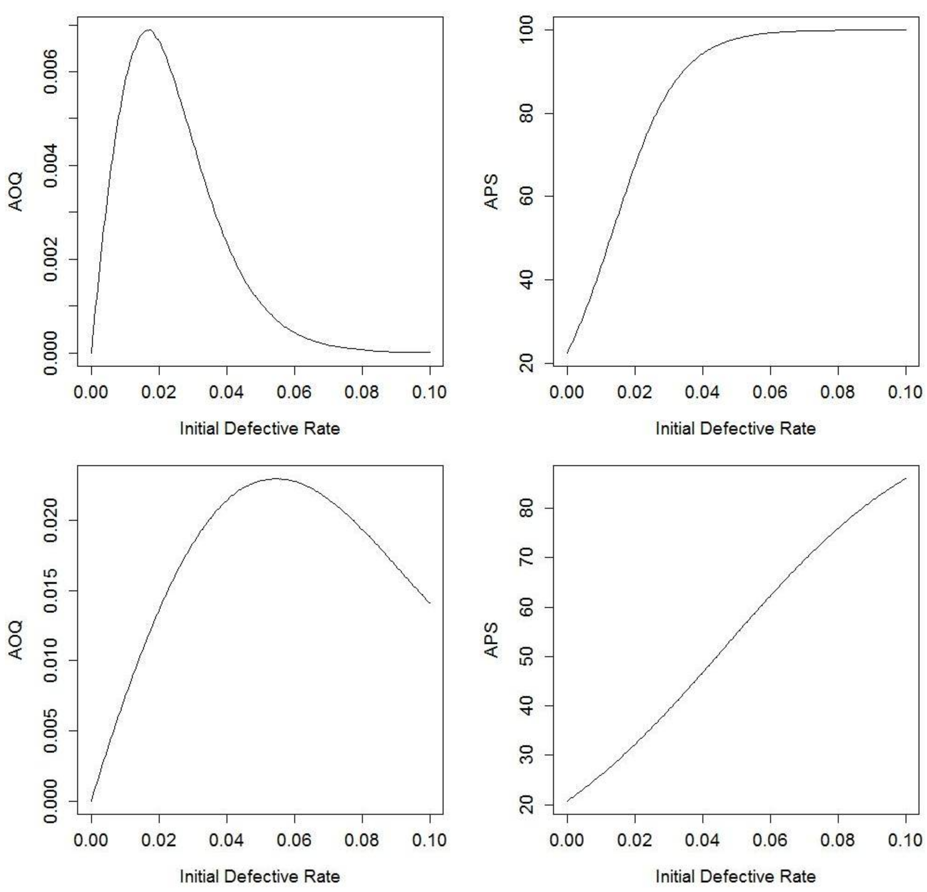
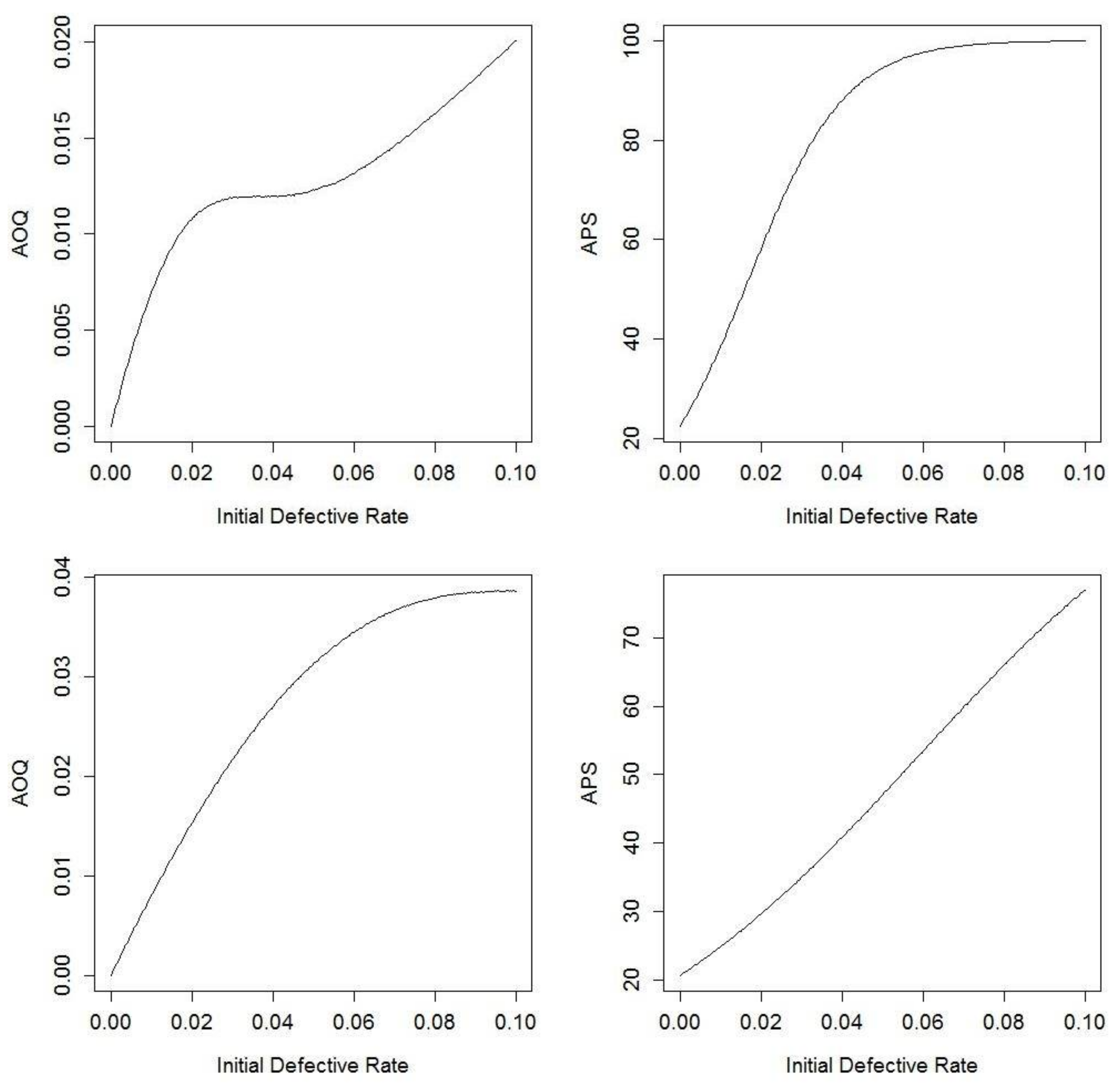
5.2. Illustrations

In this section, we revisit the analysis of Plan 1 with perfect testing. Table 3 compares the output of the simulation for AOQ and APS with the approximations in Section 5.1 and with analytical formula available in the previously discussed references.

Table 3. Plan 1 with perfect testing.

Metric	Simulation	Section 5.1 Approximation	Formulas in References [3,4]
AOQ	0.66%	0.69%	0.65%
APS	67.38%	65.34%	67.27%

The calculation using the Section 5.1 formula is close to the calculation of the simulation because F/N is small. The simulation results agree nicely with the analytical formulas available in the literature that can be used in short-run contexts provided there is perfect testing.

As a second illustration we revisit the analysis of Plan 1 with imperfect testing. Table 4 compares the output of the simulation for AOQ and APS with results obtained from naively using the imperfect testing formulas in [2]. The naiveté results from ignoring the effect of the short-run context, since the formulas in [2] are valid only under long-run contexts.

Table 4. Plan 1 with imperfect testing.

Metric	Simulation	Formulas in Reference [2]
AOQ	1.07%	1.11%
APS	58.15%	55.6%

The differences in the results shown above expose the fact that even in relatively large batches, the naïve use of the formulas in [2] can lead to non-trivial discrepancies with the correct simulation answers. As a sensitivity study, we evaluated a modification where the batch size was doubled to 6400 and the number of failures was also doubled to 128 (preserving the initial 2% probability of a defect). With the larger batch size, the short-run context becomes closer to a long-run context and the simulation estimates of AOQ and APS change to 1.09% and 56.94%, respectively, which are closer to the results given by the long-run formulas.

6. Summary

CSP-1 was designed under the assumption that the number of items to be inspected was infinitely large, as in a production line assembly context, for example. In addition, an implicit assumption of perfect testing was made. While subsequent research separately relaxed the infinite batch size and perfect testing assumption, to our knowledge our work is the first that simultaneously relaxes these two assumptions. Our research developed a simulation algorithm, and implemented it in the R programming language, for CSP-1 plans in short-run contexts and in the presence of imperfect testing. One of the outputs of the R code is the distribution of the number of failed items in the batch that escape detection, which is a performance measure that has not been studied in previous literature.

We illustrated the simulation algorithm by comparing two alternative CSP-1 designs that were of interest to the United States Navy for batch sizes of 3200. The two plans differed in the length of the required run under 100% Inspection before switching to reduced inspection (n = 100 versus n = 30, respectively). If perfect testing is assumed, the trade-off is that Plan 2 reduces the amount of sampling by about 50%, but also approximately doubles the AQO from 0.66% to 1.36%. The decision-maker at the Navy will judge if 1.36% is still an acceptable level of quality, and if so, the benefit of Plan 2 in terms of less testing effort is very compelling.

Comparing the two plans under 80% test effectiveness shows that Plan 2 offers a similar reduction in the amount of sampling, but the impact of imperfect testing is more noticeable for Plan 1 where the AOQ increases by 62% compared to an increase of 12% for Plan 2. The reason for the bigger impact on Plan 1 is because more items are tested and therefore more failed items escape as a result of the imperfect test.

For future work, an analytical analysis of CSP-1 plans with imperfect testing and in short-run contexts would be interesting. The simulation algorithm could be modified to include other types of CSP plans and a detailed comparison could be carried out, including a comparison with single-stage sampling plans.

References

- Dodge, H.F. A Sampling Inspection Plan for Continuous Production. Ann. Math. Stat. 1943, 14, 264–279. [Google Scholar] [CrossRef]
- Case, K.E.; Bennett, G.K.; Schmidt, J.W. The Dodge CSP-1 Continuous Sampling Plan under Inspection Error. AIIE Trans. 1973, 5, 193–202. [Google Scholar] [CrossRef]
- Blackwell, M.T.R. The Effect of Short Production Runs on CSP-1. Technometrics 1977, 19, 259–262. [Google Scholar] [CrossRef]
- Chen, C.H. Average Outgoing Quality Limit for Short-Run CSP-1 Plan. Tamkang J. Sci. Eng. 2005, 8, 81–85. [Google Scholar]
- Wang, R.C.; Chen, C.H. Minimum Average Fraction Inspected for Short-Run CSP-1 Plan. J. Appl. Stat. 1998, 25, 733–738. [Google Scholar] [CrossRef]
- Yang, G.L. A Renewal-Process Approach to Continuous Sampling Plans. Technometrics 1993, 25, 59–67. [Google Scholar] [CrossRef]
- Liu, M.C.; Aldag, L. Computerized Continuous Sampling Plans with Finite Production. Comput. Ind. Eng. 1993, 25, 4345–4448. [Google Scholar] [CrossRef]
- Dodge, H.F.; Torrey, M.N. Additional Continuous Sampling Inspection Plans. Ind. Qual. Control 1951, 7, 7–12. [Google Scholar] [CrossRef]
- Suresh, K.K.; Nirmala, V. Comparison of Certain Types of Continuous Sampling Plans (CSPs) and its Operating Procedures—A Review. Int. J. Sci. Res. 2015, 4, 455–459. [Google Scholar]