Article

A Gradient-Based Cuckoo Search Algorithm for a Reservoir-Generation Scheduling Problem

1
School of Hydropower and Information Engineering, Huazhong University of Science and Technology, Wuhan 430074, China
2
Hubei Key Laboratory of Digital Valley Science and Technology, Huazhong University of Science and Technology, Wuhan 430074, China
3
China Institute of Water Resources and Hydropower Research, Beijing 100038, China
4
Changjiang River Scientific Research Institute, Changjiang Water Resources Commission of the Ministry of Water Resources of China, Wuhan 430010, China
*
Author to whom correspondence should be addressed.
Algorithms 2018, 11(4), 36; https://doi.org/10.3390/a11040036
Submission received: 22 January 2018 / Revised: 11 March 2018 / Accepted: 20 March 2018 / Published: 25 March 2018

Abstract

:
In this paper, a gradient-based cuckoo search algorithm (GCS) is proposed to solve a reservoir-scheduling problem. The classical cuckoo search (CS) is first improved by a self-adaptive solution-generation technique, together with a differential strategy for Lévy flight. This improved CS is then employed to solve the reservoir-scheduling problem, and a two-way solution-correction strategy is introduced to handle variants’ constraints. Moreover, a gradient-based search strategy is developed to improve the search speed and accuracy. Finally, the proposed GCS is used to obtain optimal schemes for cascade reservoirs in the Jinsha River, China. Results show that the mean and standard deviation of power generation obtained by GCS are much better than other methods. The converging speed of GCS is also faster. In the optimal results, the fluctuation of the water level obtained by GCS is small, indicating the proposed GCS’s effectiveness in dealing with reservoir-scheduling problems.

1. Introduction

The penetration of renewable power generation has increased substantially in recent years [1]. The use of renewable energy such as wind power and hydropower can reduce greenhouse gas emissions from fossil fuels. Wind power is one of the fastest-growing sources, however it is uncertain and cannot be scheduled due to its intrinsic dependence on varying weather conditions over many years [2,3]. Solar power is less uncertain, but has higher variability compared to wind power [4]. Unlike wind energy, hydropower can be scheduled and has already played an important role in electricity supply all over the world. The long-term hydropower-generation scheduling (LHGS) of cascade reservoirs is of great importance to improving power grid stability. A suitable scheduling scheme can effectively increase the economic benefit of cascade reservoirs. The purpose of LHGS is to determine the water release of all reservoirs in a time period in order to maximize the benefit [5].
Many studies have been carried out [6,7,8] indicating that the LHGS is a non-linear and non-convex problem with very complicate constraints including water balancing, hydraulic connection, water-level limitations, water-release limitations and output capacity limitations [9]. In order to solve this problem, classical studies have taken many kinds of approaches, including dynamic programming (DP) [10,11], linear programming (LP) [12,13], the progressive optimality algorithm (POA) [14,15], and discrete differential dynamic programming (DDDP) [16,17]. However, these methods have their own shortcomings in dealing with the problems of large-scale cascade reservoirs [18].
In recent years, meta-heuristic algorithms have been popular in the search for a global optimum in non-convex problems [19]. Metaheuristics and their applications have wide application in artificial intelligence, e.g., water-distribution systems [20], transit network design problems [21], reservoir-operation optimization [22], and so forth. Many metaheuristics have included some form of stochastic optimization, so the searching efficiency is affected by the set of random variables generated [23]. By searching over a large numbers of feasible solutions, metaheuristics can often find good solutions near to the optimum solution with less computational effort [24].
Cuckoo search (CS) is one kind of metaheuristics developed by Xin-she Yang and Suash Deb in 2009 [25]. It was inspired by the behavior of some cuckoo species by laying eggs in the nests of other host birds. Compared to other artificial intelligence algorithms such as the genetic algorithm (GA) [26] and particle swarm optimization (PSO) [27], CS has the characteristics of higher solution quality, shorter computational time, and higher success rates [28]. It has been applied to various optimization problems. For example, Maiya Din et al. introduced it for the analysis of linear feedback shift register-based cryptosystems [29], Bhateja et al. used CS for the cryptanalysis of vigenere [30], Naik et al. used CS for intrinsic discriminant analysis-based face recognition [31].
Although CS has shown its advantages and has wide application in many areas, it still has some drawbacks. Proper computational time cannot be guaranteed in large-scale systems [32]. In this paper, some improvements are proposed to the original CS using four strategies: (1) a dynamic parameter adjustment of the parameter; (2) a boundary value perturbation strategy for boundary value adjustment; (3) a differential strategy for Lévy flight; (4) a different way to update solutions. When applying CS to the LHGS problem, we find that the converge speed and the results are not satisfactory. What’s more, solutions generated by a random search have the characteristic of large fluctuations in water level. Thus, a gradient strategy is designed especially for the LHGS problem. This gradient strategy improves the local search ability of the algorithm by fine-tuning the water level process. In case studies, comparisons of benchmark function tests among different algorithms has been carried out. Results show that the improved cuckoo search (ICS) performs much better than the improved harmony search (IHS) and CS. Finally, a case study of the Jinsha River is put forward to show the application of the LHGS model. The advantage of the proposed GCS is very obvious: it can effectively obtain satisfactory results in all wet years, normal years and dry years.
This paper is organized as follows: Section 2 describes the objective function and constraints of LHGS model; Section 3 gives the details of improved CS; Section 4 presents the gradient-based CS algorithm for LHGS; Section 5 is the experiments and the case study in the Jinsha River; and Section 6 is the summary of this paper.

2. Reservoir-Scheduling Problem

The main purpose of LHGS is to improve the power generation of cascaded reservoirs. The objective function can be listed as follows.

2.1. Long-Term Hydropower-Generation Scheduling (LHGS) Model

The LHGS model is used to find a set of water releases or storage volumes that maximizes the generating benefit for cascade hydropower system. The objective formula of hydropower optimization problem is given as follows:
E = max t = 1 T i = 1 N k i Q i , t H i , t Δ t
where E is the total energy production of the cascade hydropower system; T is the count of periods; N is the number of reservoirs; ki is the output coefficient of reservoir i; Qi,t is the generation flow which outflows through hydropower units of the reservoir i in time t; Hi,t is the net water head of hydropower reservoir i in time t; and ∆t is the length of time interval.

2.2. Constraints

To complete the scheduling model, the constraints of the scheduling problem are defined as:
(1) Hydraulic Connection
{ I i , t = O i 1 , t + R i , t O i 1 , t = Q i 1 , t + S i 1 , t
Ii,t is the inflow of reservoir i in time t; Oi−1,t is the outflow of reservoir i − 1 in time t; Ri,t is the interval inflow between reservoir i − 1 and i; Si−1,t is spillage of the upstream reservoir i − 1; Qi−1,t is the generation flow of the upstream reservoir i − 1.
(2) Water-Balance Constraint
V i , t = V i , t 1 + ( I i , t O i , t ) Δ t
Vi,t is the reservoir storage of reservoir i in time t.
(3) Water-Level Constraints
Z i , t min Z i , t Z i , t max
| Z i , t Z i , t 1 | Z i , t s t e p
Z i , t m i n and Z i , t m a x are, respectively, the lower and upper bounds of the water level; Z i s t e p is the limitation of water-level variation.
(4) Outflow Constraint
O i , t min O i , t O i , t max
O i , t m i n and O i , t m a x are, respectively, the minimum and maximum outflows of reservoir i.
(5) Output Constraint
N i , t min N i , t N i , t max
N i , t m i n and N i , t m a x are, respectively, the minimum and maximum power output of reservoir i.
(6) Boundary Condition
Z i , 0 = Z i , s t a r t , Z i , T = Z i , e n d
Z i , s t a r t and Z i , e n d are, respectively, the initial and terminal water levels of reservoir i.

3. Cuckoo Search Algorithm

3.1. Basic Cuckoo Search Algorithm

Cuckoo search (CS) is a meta-heuristic algorithm inspired by the obligate brood parasitism of some cuckoo species [25]. It is a population-based evolutionary algorithm and can be applied for various optimization problems. The procedures of CS are explained as follows:
  • Each cuckoo lays one egg at a time, and dumps its egg in randomly chosen nest;
  • The best nests with a high quality of eggs will carry over to the next generation;
  • The number of available host nests is fixed, and the egg laid by a cuckoo is discovered by the host bird with a probability pa. Discovering operates on some set of the worst nests, and discovered solutions are dumped from further calculations.
For a minimum function, the basic steps of the CS are summarized as the pseudo code in Algorithm 1:
Algorithm 1. Cuckoo search via Lévy flights
Objective function f ( x ) , x = ( x 1 , ... , x d ) T
Generate initial population of n host nests x i ( i = 1 , 2 , ... , n )
While (t < MaxIteration) or (stop criterion)
 Get a cuckoo i randomly by Lévy flights and evaluate its fitness
 Choose a nest j among n randomly
If f ( x i ) < f ( x j )
  Replace x j by the new solution x i
End if
If r a n d ( 0 , 1 ) < p a
  Init the worst nest x w o r s t
End if
If f ( x i ) < f ( x b e s t )
  Replace x b e s t by x i
End if
End while

3.2. Improvement for Cuckoo Search Algorithm

The basic cuckoo search algorithm (CS) is capable of finding the optimum function, but after several iterations, we found that it still needs improvements. In this section, three strategies are presented to improve the CS.

3.2.1. Dynamic Parameter Adjustment Strategy

In the CS algorithm, the abandonment of the nest is determined by its abandon probability pa. If pa is large, this nest is considered as a bad solution and would be replaced with new randomly generated solutions. The converging speed of the algorithm will decline due to the replacement, but the population diversity can be improved. If pa is small, the characteristics of the population can be reserved and it can benefit the convergence. According to this feature, a dynamic adjustment strategy is introduced to decide pa showing as Equation (9). With this strategy, there would be better global search capabilities in the early stage evolution, and the convergence becomes faster in the later stage:
p a = p a s + ( p a e p a s ) × C E N E
where CE is the current evaluation times; NE is the maximum evaluation times; and p a s and p a e are start and end p a , respectively.

3.2.2. A Boundary Value Perturbation Strategy

When a new solution is generated, the values of some dimensions may be no longer in the proper range. The common method is to adjust it to the boundary value, which may result in unexpected accumulation of solutions on the border. Thus, a boundary value perturbation strategy is carried out, as shown in Equation (10):
x i d ( t ) = { U B d r a n d ( 0 , 1 ) × mod ( x i d ( t ) U B d , U B d L B d ) ,   if   x i d ( t ) > U B d L B d + r a n d ( 0 , 1 ) × mod ( L B d x i d ( t ) , U B d L B d ) ,   if   x i d ( t ) < L B d  
where mod ( a ,   b ) is modulo operation to find the remainder after division of a by b; and UBd and LBd are the upper and lower boundary limits, respectively.

3.2.3. Differential Strategy for Lévy Flight

In CS, an important problem is the implementation of Lévy flights, as shown in the original paper [25]:
x i t + 1 = x i t + α L e v y ( λ )
Unfortunately, the original paper only described the basic idea of Lévy flights, and the details of its implementation were not given. Later studies had different interpretations of Lévy flight such as [33,34]. In this paper, the strategy used for Lévy flight is given as:
x i d = x i d + ( s l × L e v y ( u , c ) × ( x j d x i d ) )
where i and j are the numbers of randomly chosen nests; sl is the step size parameter; Levy(u,c) is sample value from the Lévy distribution, and its probability density function is:
f ( x ) = c 2 π e c 2 ( x u ) ( x u ) 3 / 2

3.2.4. Solution Updates Strategy Changes

The CS generates new solutions by Lévy flights and compares it with another randomly chosen nest. However, when replacing the randomly chosen solution, the source solution and the target solution are not relevant, so the useful information from the target solution is missing. Thus, if the new generated solution is better, instead of replacing another randomly chosen nest, we replace the source nest that is used for performing Lévy flights.
Additionally, in the proposed algorithm, the guide information from the best solution or current best solution is not used, and we should not find the optimal solution in each iteration.

3.3. Implementation of Improved Cuckoo Search (ICS)

With the improvements above, the improved CS can be described as follows:
Step 1 Initialize the algorithm parameters
This step specifies the desired parameters, including size of population (ns), abandon probability (pa), disturbance weight (w), step size (sl), and Lévy distribution parameters u and c.
Step 2 Initialize the population
In this step, new random nests ( x 1 , ... , x n s ), whose total number is ns, are generated as in Equation (14):
x i d = ( U B d L B d ) r a n d ( 0 , 1 ) + L B d , d = 1 , 2 , ... , D
Then each vector will be evaluated by the objective function and stored in the population.
Step 3 Generate a new solution by Lévy flights
Here a source nest x i and target nest x j from the population are randomly chosen. A new cuckoo from nest i flight to nest j obeys the features of Lévy flight. Then a new solution is generated from Equation (12).
If the new generated solution is out of proper range, we would adjust the solution from Equation (10).
Step 4 Update the host nest
Evaluate the fitness of the new solution f ( x i ) and compare it with the fitness of source nest f ( x i ) . If the new solution is better, replace the source nest with the new solution.
Step 5 Abandon the worst nest
If the random value is smaller than pa, a new solution is generated randomly and it will replace the worst nest.
Step 6 Check the stop criterion
Repeat Step 3 to Step 5 until the termination criterion is satisfied. In this paper, the termination criterion is the maximum number of evaluation times.
The pseudo-code of the ICS algorithm is presented in Algorithm 2.
Algorithm 2. Improved cuckoo search
Objective function f ( x ) , x = ( x 1 , ... , x d ) T
Initialize default parameters
Generate initial population of n host nests x i ( i = 1 , 2 , ... , n )
While (t < MaxEvaluation) or (stop criterion)
 Select two solution x i , x j from host nests randomly
For d=1,...,D do
   x i d = x i d + ( s l × L e v y ( u , c ) × ( x j d x i d ) )
End for
If f ( x i ) < f ( x i )
  Replace x i by the new solution x i
End if
If r a n d ( 0 , 1 ) < p a
  Init the worst nest x w o r s t
End if
End while

4. Gradient Cuckoo Search for Reservoir Scheduling

Generally, when the heuristic algorithm is applied on the reservoir-scheduling problem, the process of water levels is selected as the decision variable, as shown in Equation (15):
X = [ X 1 X 2 X N ] = [ x 1 1 , x 1 d , x 1 T x 2 1 , x 2 d , x 2 T x N 1 , x N d , x N T ]
where N is the number of reservoirs; and T is the number of time intervals.

4.1. Constraints Handling

Cascade reservoir operation is a complicated optimization problem with varieties of constraints. According to ICS, the initial population is generated following Equation (16):
x i = x i min + r a n d ( x i max x i min )
where x i m i n and x i m a x are, respectively, the lower and upper boundaries limit of reservoir i; and rand is a random number between 0 and 1. However, there is a high probability that the randomly generated solutions do not satisfy all the constraints displayed in Section 2.2. In the initialization stage, if the generated solution is not feasible, it needs to be replaced by a new feasible solution.
In the random search stage, the newly generated unfeasible solution cannot be discarded. It is adjusted to the feasible range as follows:
x i + 1 = { x i + 1 min , i f   x i + 1 < x i + 1 min x i + 1 max , i f   x i + 1 > x i + 1 max
The feasible range of water level xi+1 is defined as:
x i + 1 max = min ( x i + Δ z , Z ( x i , Q i min ) , Z ( x i , Q i P min ) , z max )
x i + 1 min = max ( x i Δ z , Z ( x i , Q i max ) , z min )
Z ( x i , Q i ) = Z ( V ( x i ) + ( I i Q i ) Δ t )
where Q t m i n and Q t m a x are, respectively, the minimum and maximum outflows of the reservoir; Q t P m i n is the minimum outflow for a guaranteed output; z m i n and z m a x are minimum and maximum water levels; Δ z is the limitation of the water-level change; and Z ( V ) and V ( Z ) are the relationship between the water level and the storage.
In the adjustment of the unfeasible solutions, a two-way solution correction strategy is employed. First, the water level is adjusted to the feasible range from period 1 to T. If the correction fails at some unpredictable period, then the water level is adjusted from period T to the breakpoint. If the correction is still not successful, the solution would be considered as an infeasible solution.

4.2. Gradient-Based Search Strategy

In the random search phase, new solutions are randomly generated from the heuristics algorithms. However, after many numerical experiments, it is found that the performances of the heuristic algorithms fail to meet the requirements. On the one hand, the variance of the calculation results is large, indicating that the algorithms are not very stable. On the other hand, the converging speed of the algorithm is quite slow when dealing with the complex cascade reservoirs problem. Hence in this section, a gradient-based search strategy is designed especially for LHGS.
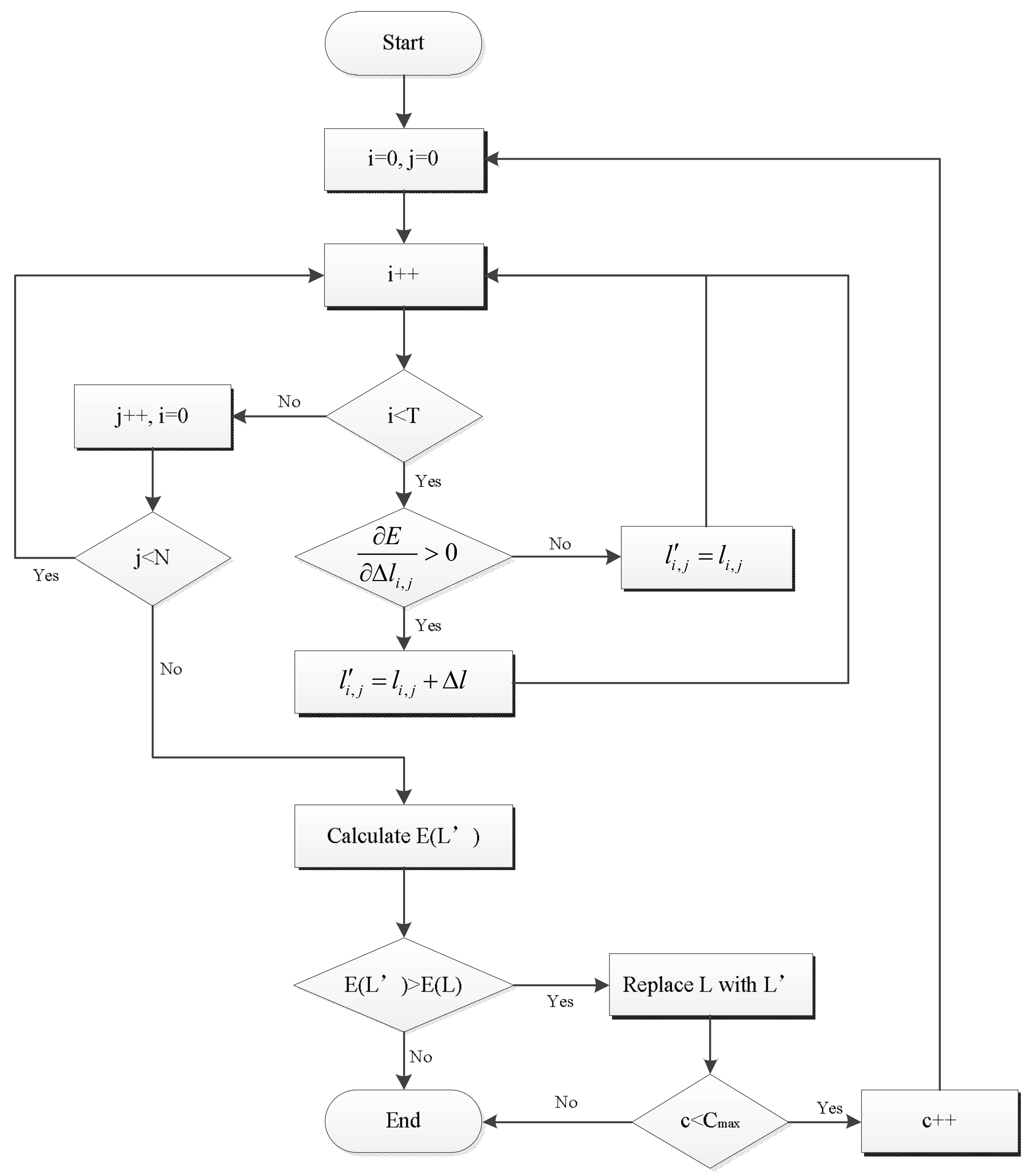
For a random generated solution, the water level is adjusted by a small gradient Δli,t as shown in Figure 1, which would result in the power generation of the entire cascade reservoir changing.
If we change the end water level of reservoir i by Δl at time period t, the power generation of reservoir i at time period t is:
{ Z i , t a d j u s t = Z i , t + Δ l Δ Q i , t = ( V i ( Z i , t + Δ l ) V i ( Z i , t ) ) / Δ T t Δ H i , t = Δ l / 2 Z d i ( Q i , t + Δ Q i , t ) + Z d i ( Q i , t ) Δ P i , t = k i ( Q i , t + Δ Q i , t ) ( H i , t + Δ H i , t ) k i Q i , t H i , t
where V i ( Z ) is the fitting function of water level and storage curve of reservoir i; and Z d i ( Q ) is the fitting function of the downstream water level and outflow curve of reservoir i.
Then the power generation of reservoir i at the next time period t + 1 can be given by:
{ Δ Q i , t + 1 = ( V i ( Z i , t ) V i ( Z i , t + Δ l ) ) / Δ T t + 1 Δ H i , t + 1 = Δ l / 2 Z d ( Q i , t + 1 + Δ Q i , t + 1 ) + Z d ( Q i , t + 1 ) Δ P i , t + 1 = k i ( Q i , t + 1 + Δ Q i , t + 1 ) ( H i , t + 1 + Δ H i , t + 1 ) k i Q i , t + 1 H i , t + 1
When the outflow of reservoir i is changed and the water level of the downstream reservoirs remains the same, the inflow of all reservoirs in the downstream reservoir would be changed by the outflow of reservoir i. For one of the reservoirs downstream, the power generation at time period t is:
{ Δ Q j , t = Δ Q i , t Δ H j , t = Z d j ( Q j , t ) Z d j ( Q j , t + Δ Q j , t ) Δ P j , t = k j ( Q j , t + Δ Q j , t ) ( H j , t + Δ H j , t ) k j Q j , t H j , t
The power generation of the next reservoir i + 1 at time period t + 1 is:
{ Δ Q j , t + 1 = Δ Q i , t + 1 Δ H j , t + 1 = Z d j ( Q j , t + 1 ) Z d j ( Q j , t + 1 + Δ Q j , t + 1 ) Δ P j , t + 1 = k j ( Q j , t + 1 + Δ Q j , t + 1 ) ( H j , t + 1 + Δ H j , t + 1 ) k j Q j , t + 1 H j , t + 1
For the solution adjustment, we need to adjust this to the better direction. Instead of a time-consuming fitness calculation of the incremental power generation ΔE, we only need to determine whether the incremental power generation ΔE is positive. If ΔE > 0, the adjustment will be made to give a better solution. Otherwise the previous solution is kept without change.
In this paper, we determine whether ΔE is positive from the calculation of the partial derivative of power generation E with respect to the gradient Δl, as given below. For the reservoir i at time period t shown in Equation (25), the partial derivative of power output is:
{ Q i , i l = lim Δ l 0 Δ Q i , t Δ l = 1 Δ T t lim Δ l 0 V i ( Z i , t + Δ l ) V i ( Z i , t ) Δ l = 1 Δ T t V i ( Z i , t ) H i , t l = lim Δ l 0 Δ l / 2 Z d i ( Q i , t + Δ Q i , t ) + Z d i ( Q i , t ) Δ l = 1 2 Z d i ( Q i , t ) Q i , t l P i , t l = k i ( Q i , t H i , t l + H i , t Q i , t l )
For the reservoir i at time period t + 1 shown in Equation (26), the partial derivative of power output is:
{ Q t + 1 l = lim Δ l 0 V ( Z t ) V ( Z t + Δ l ) Δ l Δ T t + 1 = 1 Δ T t + 1 V ( Z t ) H t + 1 l = 1 2 lim Δ l 0 Z d ( Q t + 1 + Δ Q t + 1 ) Z d ( Q t + 1 ) Δ l = 1 2 Z d ( Q t + 1 ) Q t + 1 l P t + 1 l = k ( Q t H t + 1 l + H t Q t + 1 l )
For the reservoir downstream at time period t shown in Equation (27), the partial derivative of power output is:
{ Q j , t l = Q i , t l H j , t l = lim Δ l 0 Z d j ( Q j , t ) Z d j ( Q j , t + Δ Q j , t ) Δ l = Z d j ( Q j , t ) Q j , t l P j , t l = k j ( Q j , t H j , t l + H j , t Q j , t l )
For the reservoir downstream at time period t + 1 shown in Equation (28), the partial derivative of power output is:
{ Q j , t + 1 l = Q i , t + 1 l H j , t + 1 l = Z d j ( Q j , t + 1 ) Q j , t + 1 l P j , t + 1 l = k j ( Q j , t + 1 H j , t + 1 l + H j , t + 1 Q j , t + 1 l )
According to the formulas above, the partial derivative of power generation E with respect to the gradient Δl is:
E l = Δ T t P i , t l + Δ T t + 1 P i , t + 1 l + j = i + 1 N ( Δ T t P j , t l + Δ T t + 1 P j , t + 1 l )
If E l > 0 , adjust the water level by Δl, otherwise adjustment is rejected. For the cascade system, the flowchart of the gradient-based search strategy is shown in Figure 2.

4.3. Implementation of Gradient-Based Cuckoo Search (GCS) for Long-Term Hydropower Generation Scheduling (LHGS)

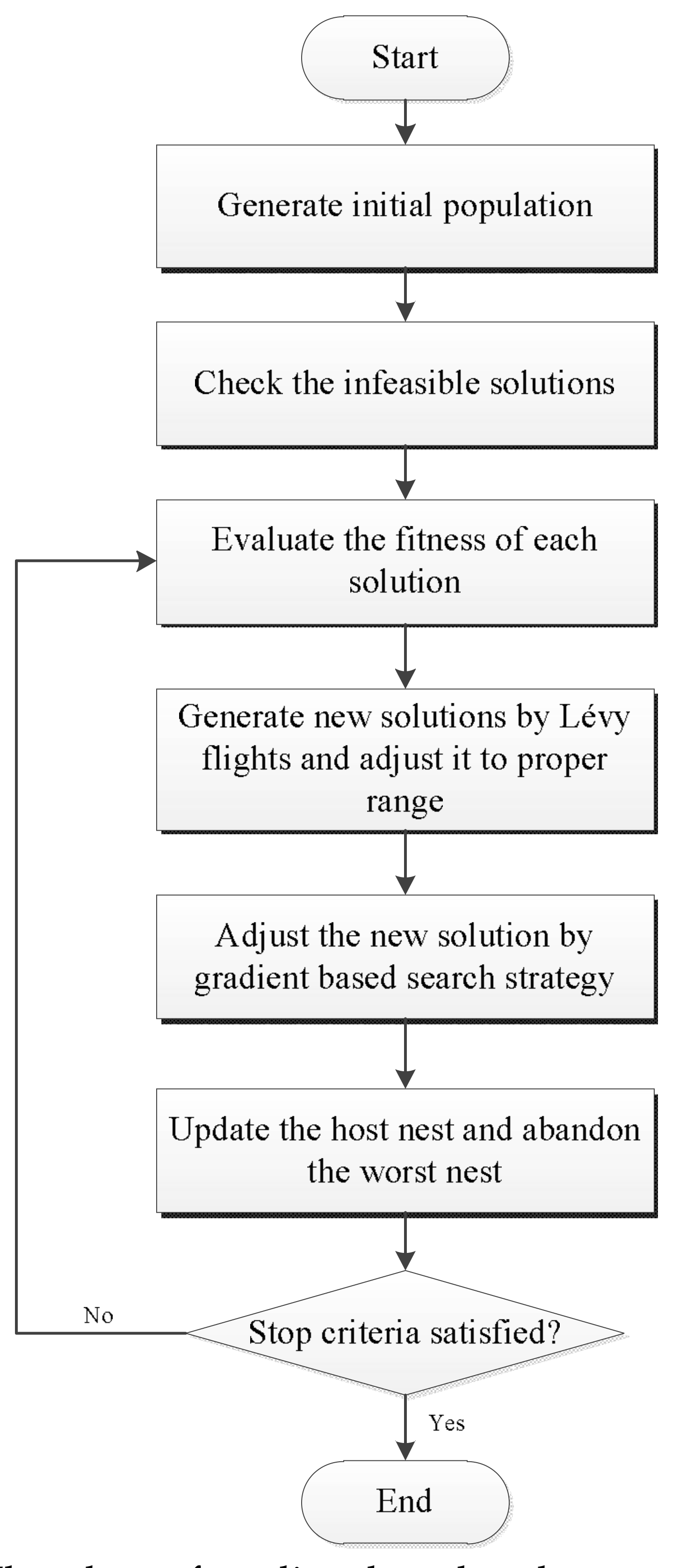
According to the description above, the steps to solve long-term scheduling problem using the cuckoo search algorithm with the gradient-based search strategy (GCS) are shown in Figure 3:
Step 1:
Randomly generate feasible initial solutions.
Step 2:
Evaluate fitness of the solutions.
Step 3:
Generate new solutions by Lévy flights.
Step 4:
If the new solution is infeasible, adjust it by two-way solution correction strategy.
Step 5:
Adjust the new solution by gradient-based search strategy.
Step 6:
Update the host nest.
Step 7:
Abandon the worst nest.
Step 8:
Repeat Steps 3 to 7 until the stop criteria is reached.

5. Case Study

5.1. Study Area

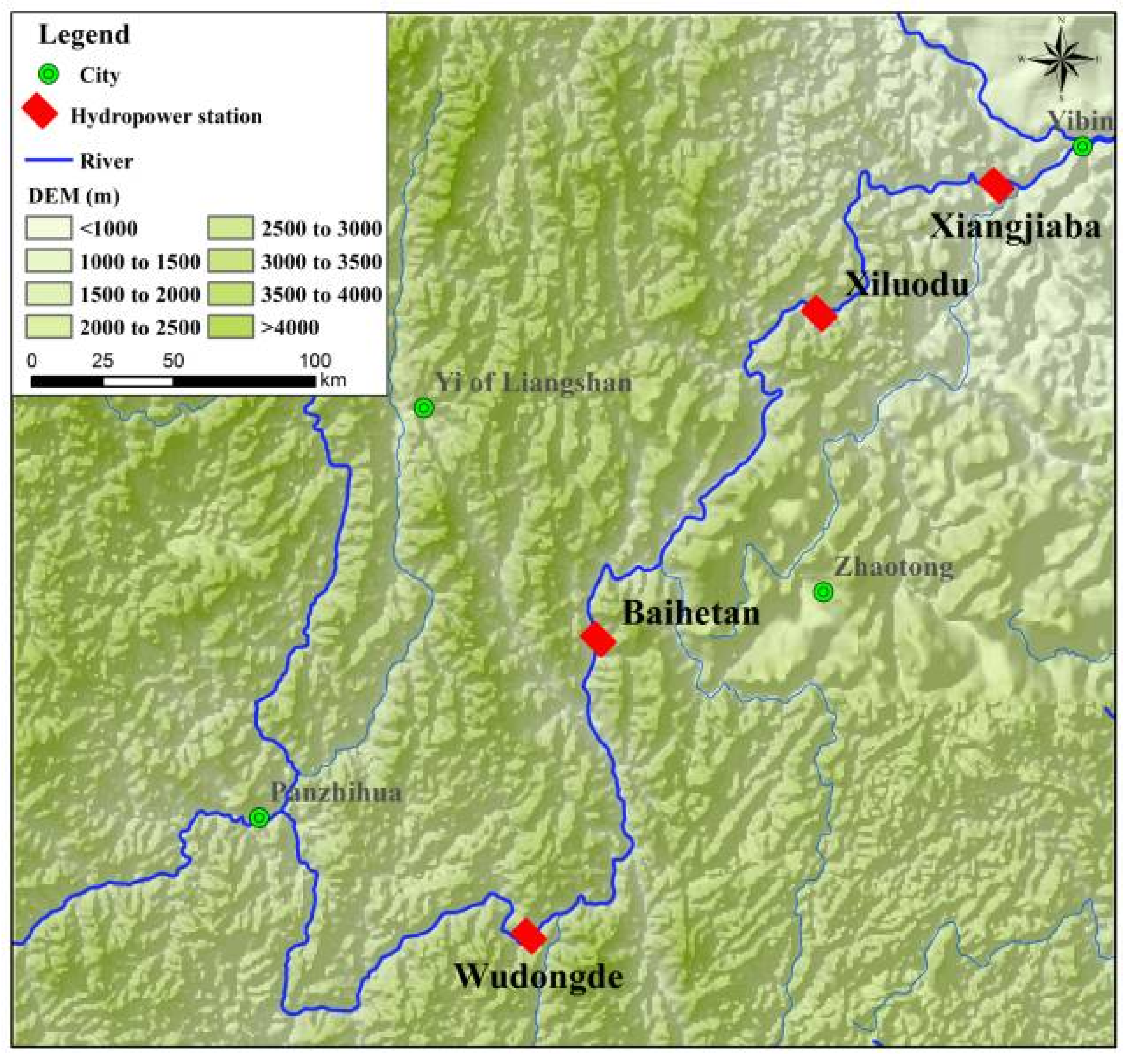
The Jinsha River is the upper reach of the Yangtze River in south-west China. It flows through Qinghai, Sichuan and Yunnan provinces. The Jinsha River is rich in water resources, and is being heavily developed for hydroelectric power. In this case study, we discuss four hydropower stations with total installed capacity of 42,960 MW on the river, including Wudongde, Baihetan, Xiluodu and Xiangjiaba. The locations of these hydropower stations are signed in Figure 4, and the major parameters of these hydropower stations are listed in Table 1.
The aim of long-term hydropower generation scheduling is to determine the water release process of all hydropower stations at each period. The total power generation of different schemes will be different, thus we need a suitable method to solve this problem. In this case, we do the scheduling simulation of the cascade hydropower stations using the proposed GCS algorithm.
The topology of the four reservoirs in the Jinsha River is shown in Figure 5. The historical observed streamflow of Pingshan hydrological station is used as the input of the LHGS model.

5.2. Benchmark Function Tests

To evaluate the performance of the proposed ICS, we chose several famous typical benchmark functions, shown in Table 2. Results obtained by proposed ICS algorithms are compared with that simulated by improved harmony search (IHS) [35], the Kbest gravitational search algorithm (KGSA) [36] and basic CS. Of the functions in Table 2, the Ackley function, Griewank function, Rastrigin function, Rosenbrock function and Happy Cat function are multimodal functions. The Sphere function, Bent Cigar function, Discus function and Schwefel 2.22 function are unimodal functions. These functions will be tested under sophisticated features such as shifted and rotated features.
Dimensions of the benchmark functions are set to 10. The maximum evaluation count is set to 100,000. The default parameters of ICS are n s = 30 , p a s = 0.3 ,     p a e = 0.1 ,   s l = 0.01 ,   u = 0 ,   c = 1.5 . The parameters of IHS and GSA are set to the default values in [35,36]. All of the experiments are performed using a computer with 2.7 GHz Intel i7-4800MQ with 8 GB RAM. The source code is compiled with Java SE8.
Table 3 shows the results of the algorithms including means and standard deviation based on 100 independent tests for each benchmark function. As demonstrated in Table 3, ICS performs superior to IHS, KGSA and CS in most functions except the shifted Rosenbrock function, shifted Happy Cat function, and rotated and shifted Ackley function. Especially on the Sphere, Bent Cigar and Discus, the means and standard deviations of ICS are extremely close to the optimal solutions, much better than other algorithms. While on Rosenbrock function, shifted Happy Cat function, rotated and shifted Ackley function, KGSA performs slightly better than ICS. Overall, ICS can find a satisfactory solution, meaning that the improvement is effective.

5.3. Reservoir Scheduling in Wet Years

To evaluate the gradient strategy for reservoir scheduling, the optimal scheduling scheme of the cascade hydropower stations were obtained by using GCS and compared with those obtained by IHS, KGSA and CS. The parameter of GCS are n s = 40 ,   p a s = 0.3 ,   p a e = 0.1 ,   s l = 0.01 ,   u = 0 ,   c = 1.5 , and the maximum evaluation times is set to 12,000. The initial and end water levels of the reservoirs are set to their normal levels as shown in Table 1. Each month is divided into three periods of approximately 10 days each, resulting in 36 time intervals in a year. Each method is run 100 times, independently.
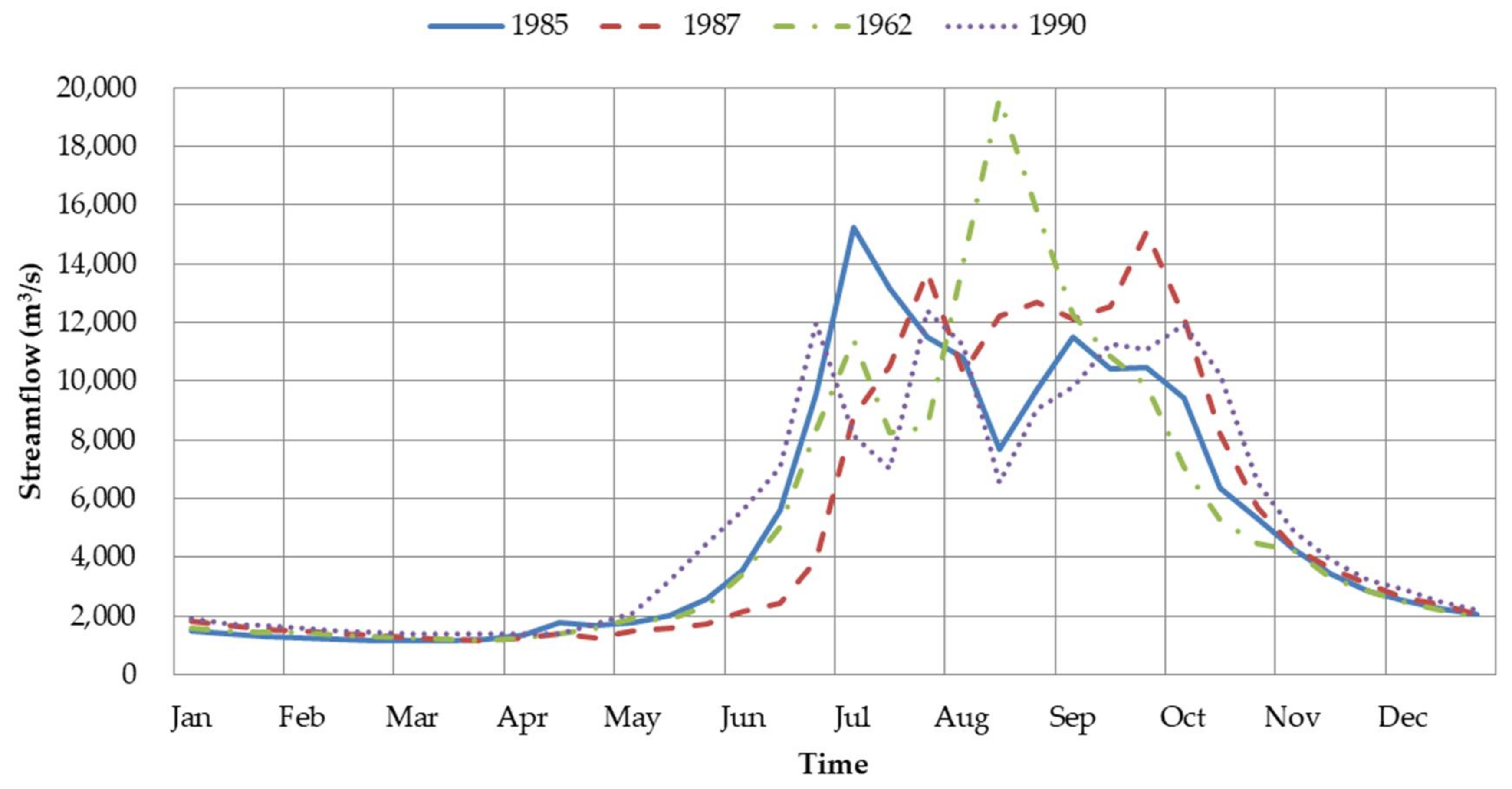
To evaluate the performance of GCS on reservoir scheduling in wet years, the streamflow of Pingshan station in Figure 6 was chosen as the input of the LHGS model. As shown in Equation (15), the water levels of the reservoirs at different time intervals are the optimization parameters. Because the water level at the 36th time interval is set to the normal water level, the optimization parameters of each reservoir are 35 and the number of reservoirs is 4, meaning that it is a 140-dimensional problem. Equation (1) is the fitness function of LHGS, and the larger power generation means a better scheduling solution.
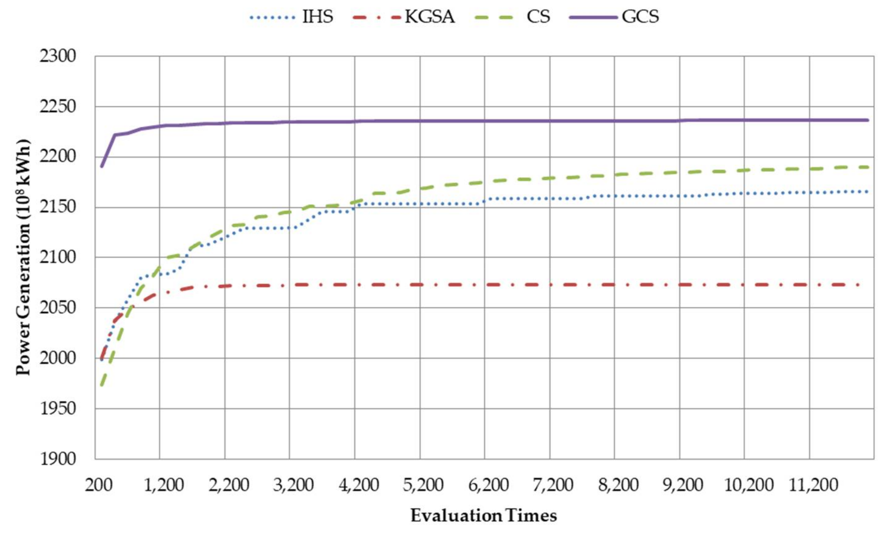
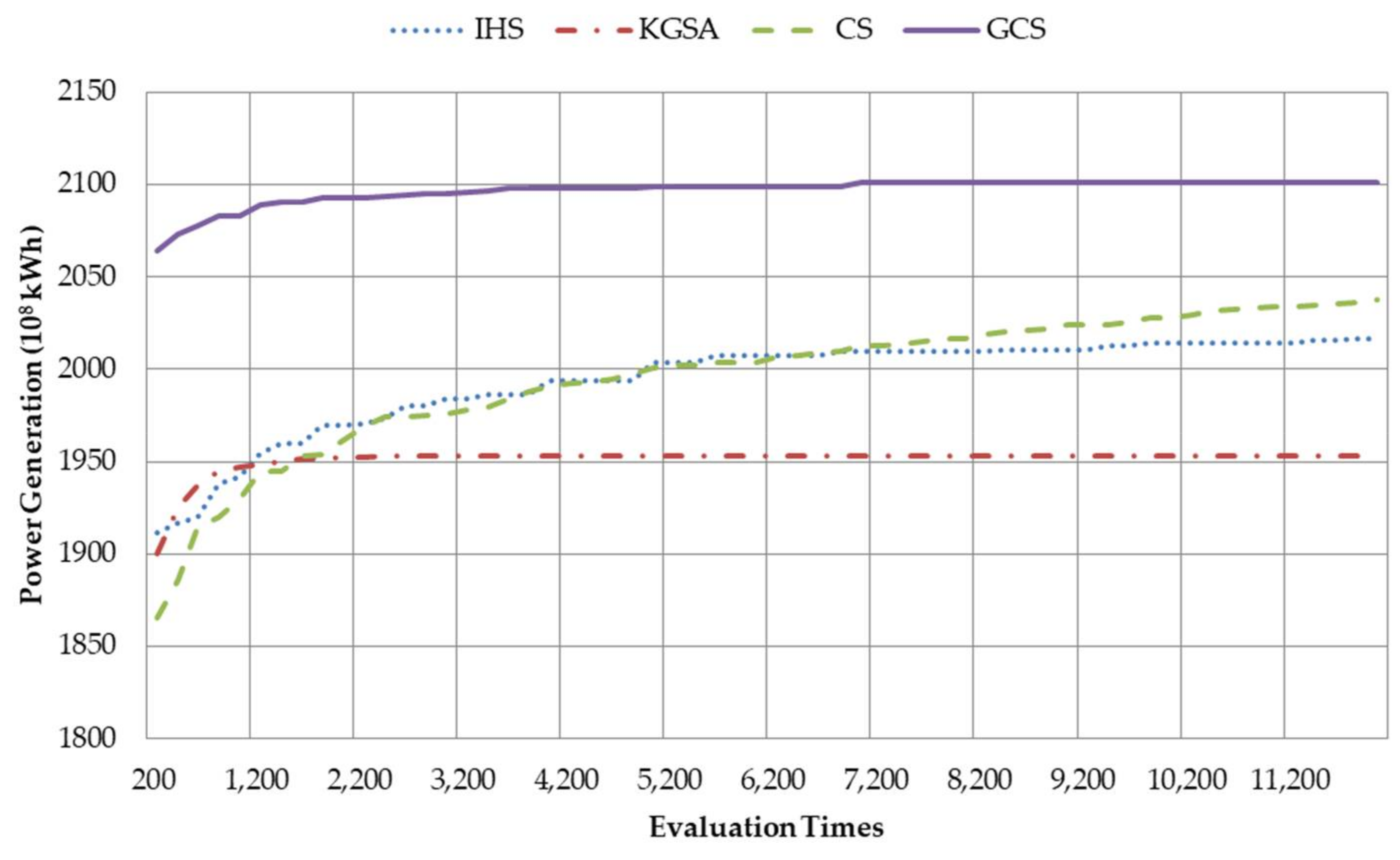
Table 4 clearly shows that GCS is superior to the other three methods. The average power generation obtained by GCS is 232.2, 223.7, 226.3 and 248.4 billion kWh in the four wet years. Compared with IHS, KGSA and CS, the average increases are 4.2%, 8.6% and 2.6%, respectively. It is also noted that the standard deviation obtained by GCS is at least 10 times smaller than that obtained by the other three methods, thus indicating GCS is more stable. Figure 7 shows the convergence process of the four algorithms in the case of the year 1987 as an example. It can be seen from Figure 7 that GCS has the fastest convergence speed, IHS and ICS have not converged yet, while KGSA has fallen into a local optimum.
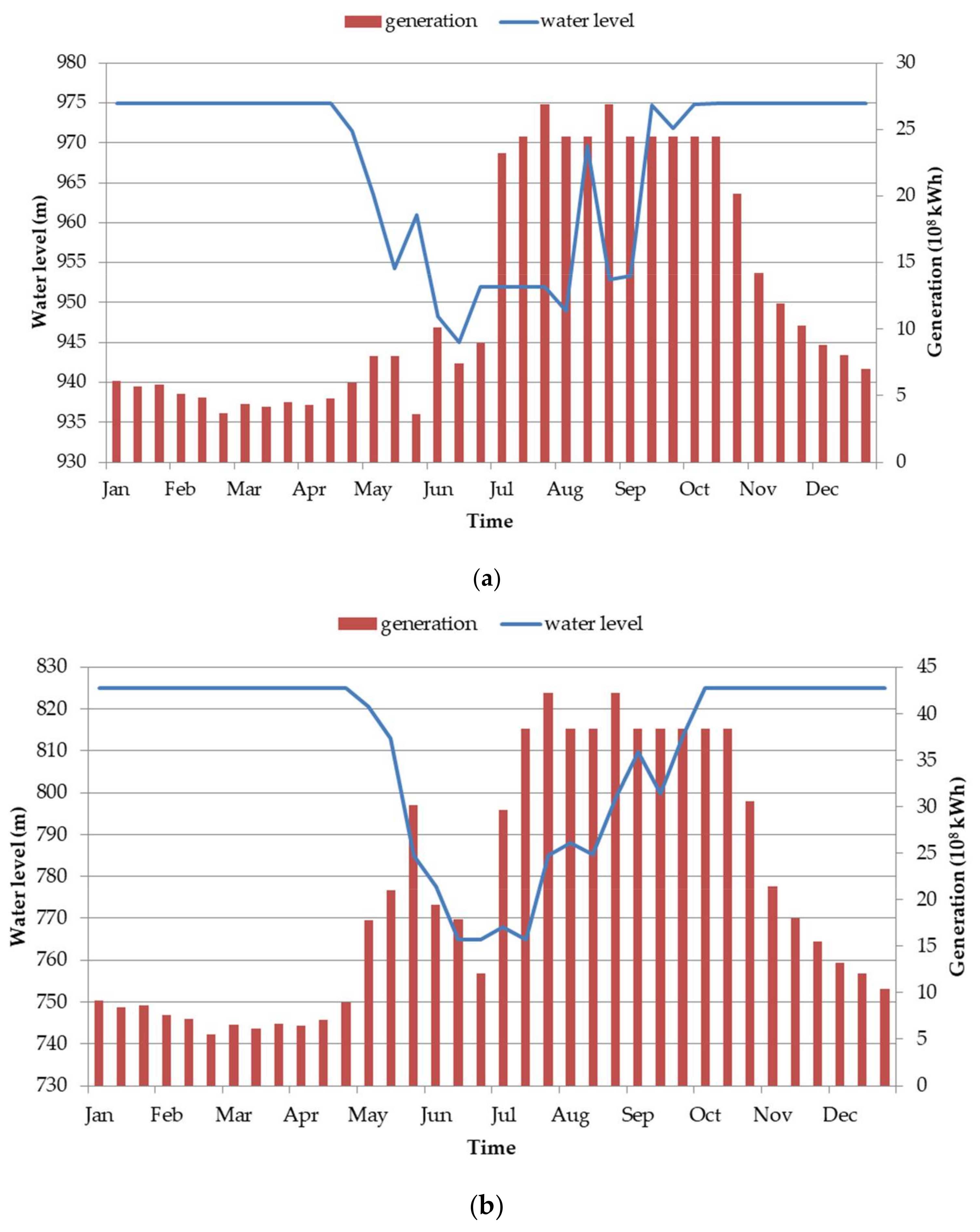
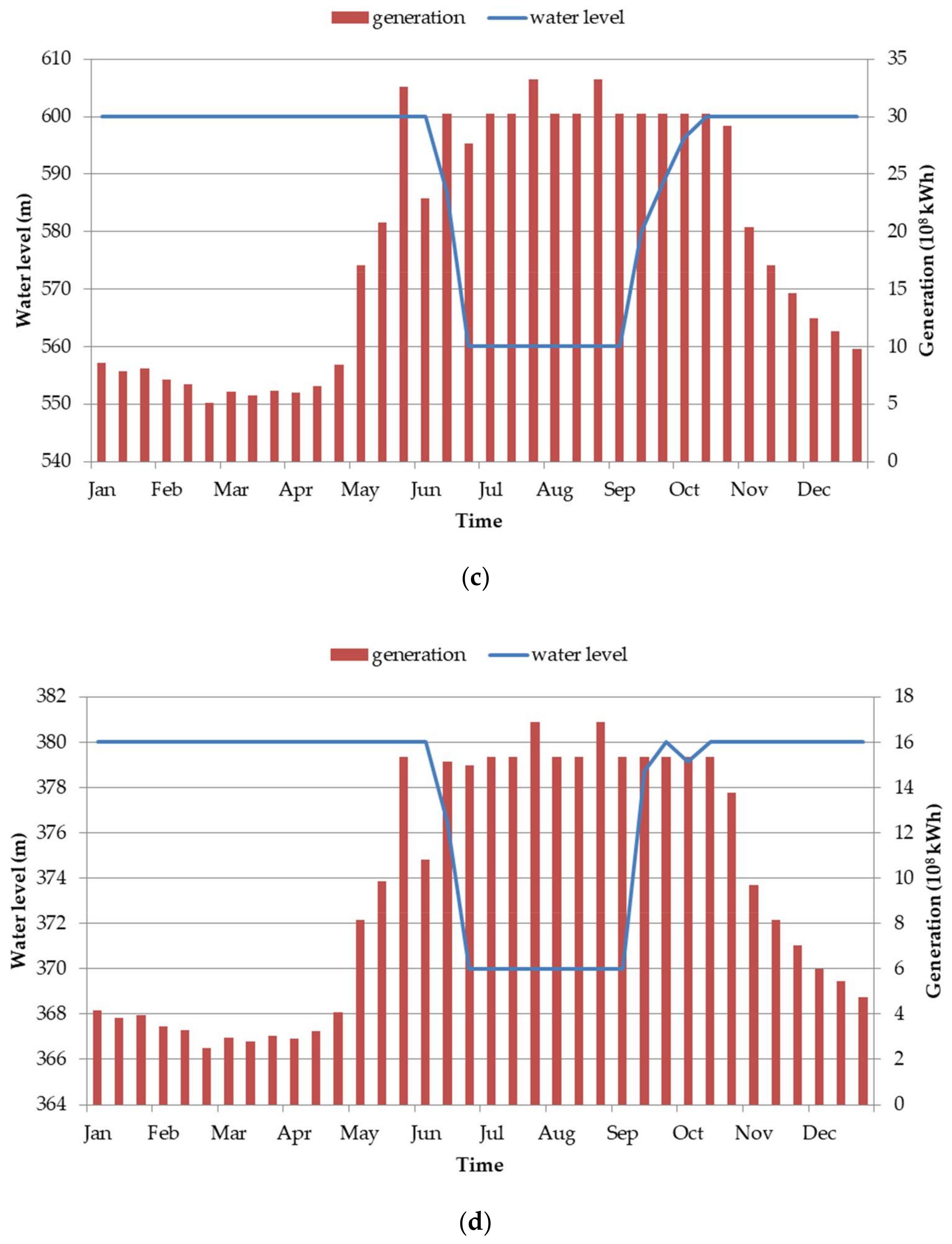
Figure 8 shows the optimal results of the four hydropower stations in the year 1987. As shown in Figure 6, the streamflow in 1987 increased significantly in July, August and September. The water levels also dropped below the flood limit water level during the flooding season. In the non-flooding season, the water levels remained at the normal level from November to March. The fluctuation of the water level obtained by GCS is small, indicating that it is an effective way to solve LHGS.

5.4. Reservoir Scheduling in Normal Years

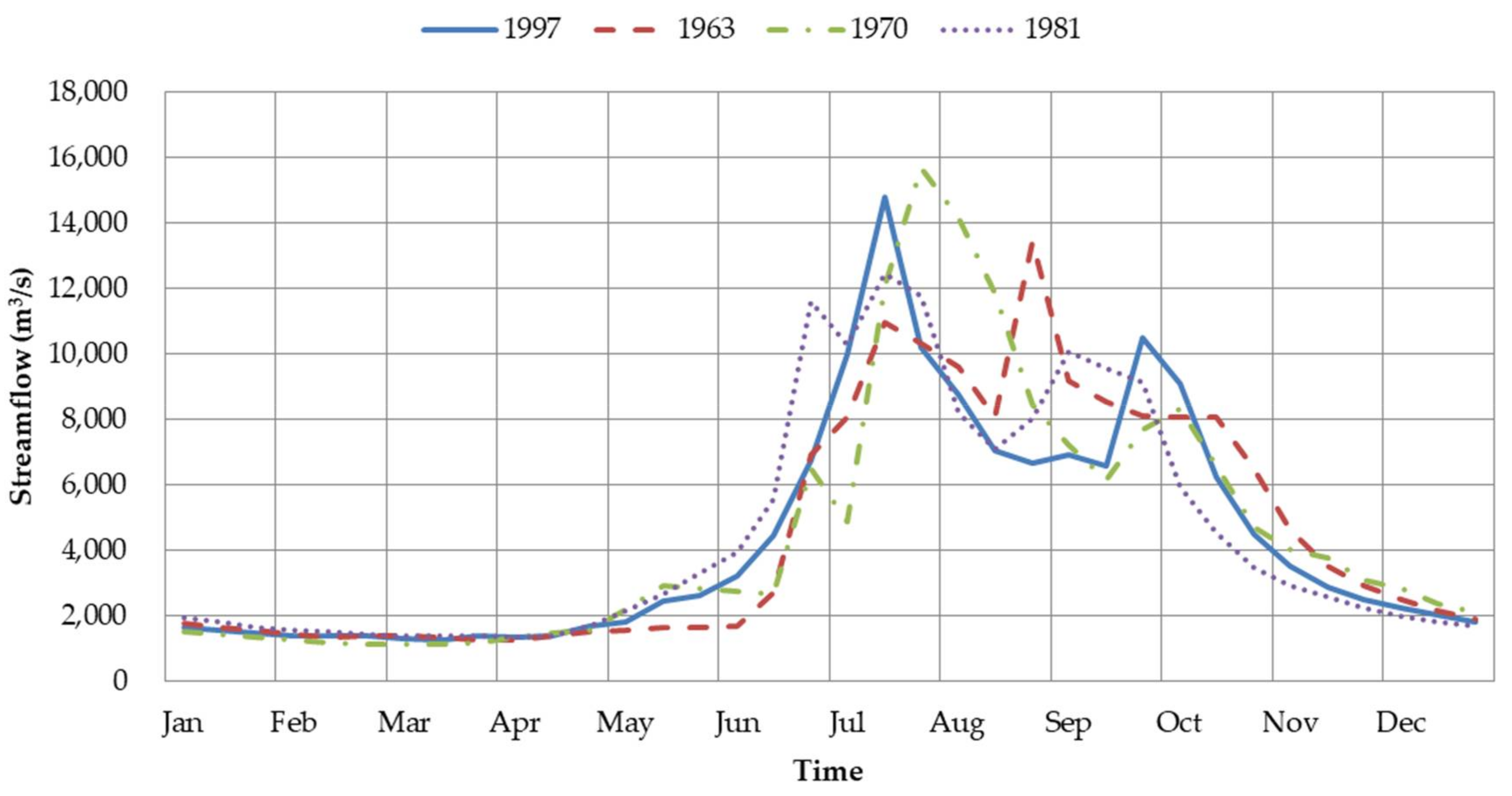
In this section, we evaluate the performance of GCS in normal years. Streamflows of the Pingshan station in Figure 9 were chosen as the input of the LHGS model. The parameters and other conditions were the same as those in Section 5.3.
As shown in Table 5, GCS gains more power generation than the other three methods. The average power generation obtained by GCS is 210.5, 220.5, 218.1 and 215.9 billion kWh in the four normal years. Compared with IHS, KGSA and CS, the average increases are 5.8%, 8.6% and 3.3%, respectively. The standard deviation obtained by GCS is also smaller than that obtained by the other three methods. Figure 10 shows the convergence process of the four algorithms in the case of the year 1997 as an example. It can be seen from Figure 10 that GCS has the fastest convergence speed. As in Section 5.3, KGSA does not perform well compared with the other methods.

5.5. Reservoir Scheduling in Dry Years

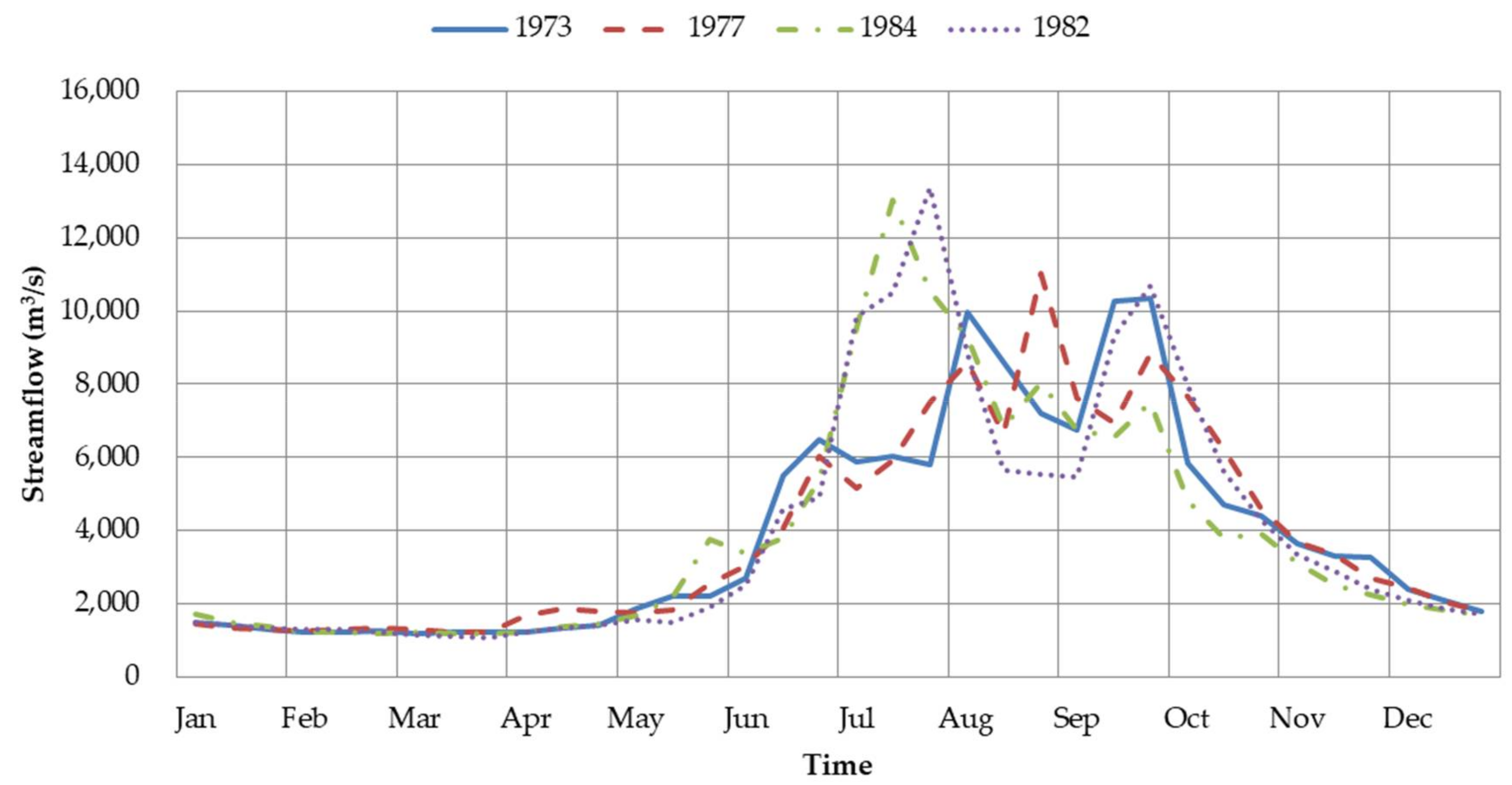
In this section, we evaluate the performance of GCS in dry years. The streamflows of Pingshan station in Figure 11 were chosen as the input of the LHGS model. The parameters and other conditions were also the same as those in Section 5.3.
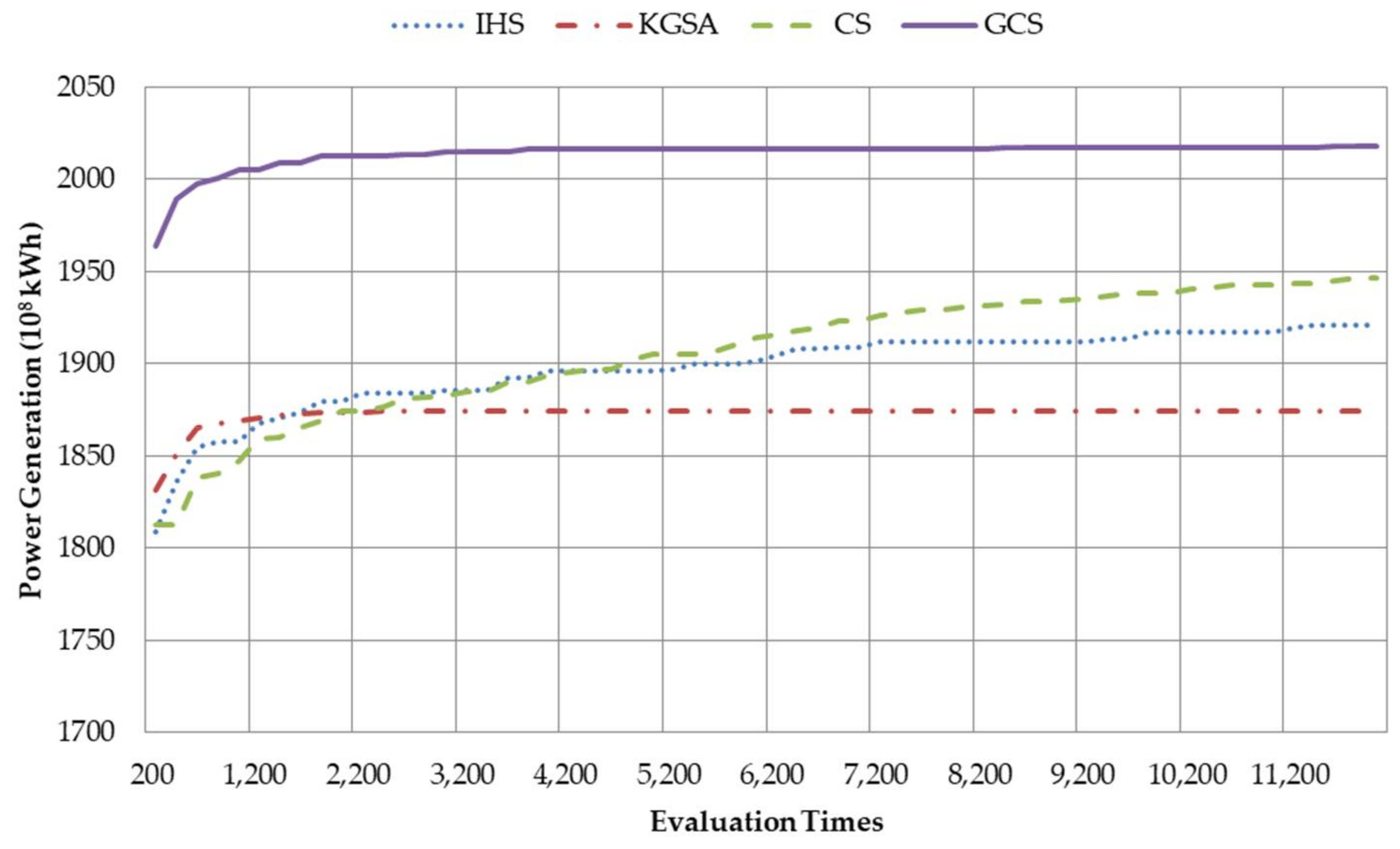
As in Section 5.3 and Section 5.4, GCS performed best in these four methods. The mean values obtained by KGSA are the smallest, while the standard deviations obtained by IHS are the largest. As shown in Table 6, the average power generation obtained by GCS is 199.2, 201.9, 194.4 and 197.7 billion kWh in the four normal years. Compared with IHS, KGSA and CS, the average increases are 5.0%, 7.7% and 3.2%, respectively. Figure 12 also shows that the convergence speed of GCS is the fastest. From Section 5.3, Section 5.4 and Section 5.5, it is clear that GCS can effectively obtain satisfactory results in different streamflow input scenarios.

6. Conclusions

The long-term hydropower generation of cascade reservoirs is one of the active research areas in water resources management. According to the operating characteristics of the reservoirs, we propose a gradient strategy to improve the performance of the cuckoo search algorithm when dealing with the LHGS problem. Moreover, the original CS algorithm is adapted with four improvements: a dynamic parameter adjustment of the parameter, a boundary value perturbation strategy for boundary value adjustment, a differential strategy for Lévy flight, and a different way to update solutions.
In the experimental work, the performance of the improvement is shown by several benchmark tests. Results show that the improved CS achieves better results than the other three methods. Finally, the improved CS is hybridized with the gradient strategy and is applied to the LHGS problem in the Jinsha River. The case study shows that the simulation results obtained by GCS are more reliable and stable than those obtained by IHS, KGSA and CS. Compared with IHS, KGSA and CS, the average increases are 4.2%, 8.6% and 2.6% in wet years, 5.8%, 8.6% and 3.3% in normal years, and 5.0%, 7.7% and 3.2% in dry years. The standard deviation obtained by GCS is smaller than that obtained by the other three methods. Overall, GCS can effectively obtain satisfactory results in different streamflow input scenarios.
However, simulation results show that ICS still has drawbacks such as local convergence when dealing with some functions. The uncertainty in reservoir generation scheduling is also not considered yet. Further research is underway to solve these problems.

Acknowledgments

This work is supported by the National Key R&D Program of China (2016YFC0402205), the Key Program of the Major Research Plan of the National Natural Science Foundation of China (No. 91547208), the National Natural Science Foundation of China (No. 51479075, No. 51409008), and the National Public Research Institutes for Basic R&D Operating Expenses Special Project (no. CKSF2017008/SZ). We also acknowledge the entire development team, without whose help this research could not have been undertaken.

Author Contributions

Yu Feng wrote the ICS and GCS algorithm. Chao Wang and Li Mo wrote the LHGS model. Jiang Wu, Zhe Yuan performed the experiments. Final checks were done by Jianzhong Zhou.

Conflicts of Interest

The authors declare no conflict of interest.

References

  1. Reddy, S.S.; Momoh, J.A. Realistic and transparent optimum scheduling strategy for hybrid power system. IEEE Trans. Smart Grid 2015, 6, 3114–3125. [Google Scholar] [CrossRef]
  2. Reddy, S.S.; Abhyankar, A.R.; Bijwe, P.R. Market clearing for a wind-thermal power system incorporating wind generation and load forecast uncertainties. In Proceedings of the 2012 IEEE Power and Energy Society General Meeting, San Diego, CA, USA, 22–26 July 2012; pp. 1–8. [Google Scholar]
  3. Reddy, S.S.; Panigrahi, B.K.; Kundu, R.; Mukherjee, R.; Debchoudhury, S. Energy and spinning reserve scheduling for a wind-thermal power system using cma-es with mean learning technique. Int. J. Electr. Power Energy Syst. 2013, 53, 113–122. [Google Scholar] [CrossRef]
  4. Reddy, S.S.; Bijwe, P.R.; Abhyankar, A.R. Real-time economic dispatch considering renewable power generation variability and uncertainty over scheduling period. IEEE Syst. J. 2015, 9, 1440–1451. [Google Scholar] [CrossRef]
  5. Liao, X.; Zhou, J.; Ouyang, S.; Zhang, R.; Zhang, Y. An adaptive chaotic artificial bee colony algorithm for short-term hydrothermal generation scheduling. Int. J. Electr. Power Energy Syst. 2013, 53, 34–42. [Google Scholar] [CrossRef]
  6. Tian, H.; Yuan, X.; Ji, B.; Chen, Z. Multi-objective optimization of short-term hydrothermal scheduling using non-dominated sorting gravitational search algorithm with chaotic mutation. Energy Convers. Manag. 2014, 81, 504–519. [Google Scholar] [CrossRef]
  7. Wang, K.W.; Chang, L.C.; Chang, F.J. Multi-tier interactive genetic algorithms for the optimization of long-term reservoir operation. Adv. Water Resour. 2011, 34, 1343–1351. [Google Scholar] [CrossRef]
  8. Zhang, H.; Zhou, J.; Fang, N.; Zhang, R.; Zhang, Y. An efficient multi-objective adaptive differential evolution with chaotic neuron network and its application on long-term hydropower operation with considering ecological environment problem. Int. J. Electr. Power Energy Syst. 2013, 45, 60–70. [Google Scholar] [CrossRef]
  9. Liao, X.; Zhou, J.; Zhang, R.; Zhang, Y. An adaptive artificial bee colony algorithm for long-term economic dispatch in cascaded hydropower systems. Int. J. Electr. Power Energy Syst. 2012, 43, 1340–1345. [Google Scholar] [CrossRef]
  10. Soares, S.; Ohishi, T.; Cicogna, M.; Arce, A. Dynamic Dispatch of Hydro Generating Units. In Proceedings of the 2003 IEEE Bologna Power Tech Conference, Bologna, Italy, 23–26 June 2003; Volume 2, p. 6. [Google Scholar]
  11. Cheng, C.T.; Liao, S.L.; Tang, Z.T.; Zhao, M.Y. Comparison of particle swarm optimization and dynamic programming for large scale hydro unit load dispatch. Energy Convers. Manag. 2009, 50, 3007–3014. [Google Scholar] [CrossRef]
  12. Tu, M.-Y.; Hsu, N.-S.; Yeh, W.W.-G. Optimization of reservoir management and operation with hedging rules. J. Water Resour. Plan. Manag. 2003, 129, 86–97. [Google Scholar] [CrossRef]
  13. Juhwan, Y. Maximization of hydropower generation through the application of a linear programming model. J. Hydrol. 2009, 376, 182–187. [Google Scholar]
  14. Nanda, J.; Bijwe, P.R. Optimal hydrothermal scheduling with cascaded plants using progressive optimality algorithm. IEEE Trans. Power Appar. Syst. 1981, PAS-100, 2093–2099. [Google Scholar] [CrossRef]
  15. Cheng, C.; Shen, J.; Wu, X. Short-term scheduling for large-scale cascaded hydropower systems with multivibration zones of high head. J. Water Resour. Plan. Manag. 2011, 138, 257–267. [Google Scholar] [CrossRef]
  16. Chow, V.T.; Maidment, D.R.; Tauxe, G.W. Computer time and memory requirements for DP and DDDP in water resource systems analysis. Water Resour. Res. 1975, 11, 621–628. [Google Scholar] [CrossRef]
  17. Cheng, C.; Wang, S.; Chau, K.W.; Wu, X. Parallel discrete differential dynamic programming for multireservoir operation. Environ. Model. Softw. 2014, 57, 152–164. [Google Scholar] [CrossRef]
  18. Wang, C.; Zhou, J.; Peng, L.; Liu, Y. Long-term scheduling of large cascade hydropower stations in Jinsha River, China. Energy Convers. Manag. 2015, 90, 476–487. [Google Scholar] [CrossRef]
  19. Beck, A.T.; Gomes, W.J.D.S. A comparison of deterministic, reliability-based and risk-based structural optimization under uncertainty. Probab. Eng. Mech. 2012, 28, 18–29. [Google Scholar] [CrossRef]
  20. Yoo, D.G. Improved mine blast algorithm for optimal cost design of water distribution systems. Eng. Optim. 2014, 47, 1602–1618. [Google Scholar]
  21. Almasi, M.H.; Sadollah, A.; Mounes, S.M.; Karim, M.R. Optimization of a transit services model with a feeder bus and rail system using metaheuristic algorithms. J. Comput. Civ. Eng. 2015, 29, 04014090. [Google Scholar] [CrossRef]
  22. Moeini, R.; Soltani-Nezhad, M.; Daei, M. Constrained gravitational search algorithm for large scale reservoir operation optimization problem. Eng. Appl. Artif. Intell. 2017, 62, 222–233. [Google Scholar] [CrossRef]
  23. Bianchi, L.; Dorigo, M.; Gambardella, L.M.; Gutjahr, W.J. A survey on metaheuristics for stochastic combinatorial optimization. Nat. Comput. 2009, 8, 239–287. [Google Scholar] [CrossRef]
  24. Blum, C.; Roli, A. Metaheuristics in combinatorial optimization: Overview and conceptual comparison. ACM Comput. Surv. 2003, 35, 268–308. [Google Scholar] [CrossRef]
  25. Yang, X.S.; Deb, S. Cuckoo search via levy flights. In Proceedings of the 2009 World Congress on Nature & Biologically Inspired Computing (NaBIC), Coimbatore, India, 9–11 December 2009; pp. 210–214. [Google Scholar]
  26. Ouyang, P.; Pano, V. Comparative study of de, pso and ga for position domain pid controller tuning. Algorithms 2015, 8, 697–711. [Google Scholar] [CrossRef]
  27. Rabanal, P.; Rodríguez, I.; Rubio, F. Parallelizing particle swarm optimization in a functional programming environment. Algorithms 2014, 7, 554–581. [Google Scholar] [CrossRef]
  28. Nguyen, T.T.; Vo, D.N. Modified cuckoo search algorithm for multiobjective short-term hydrothermal scheduling. Swarm Evol. Comput. 2017, 37, 73–89. [Google Scholar] [CrossRef]
  29. Din, M.; Pal, S.K.; Muttoo, S.K.; Jain, A. Applying cuckoo search for analysis of lfsr based cryptosystem. Perspect. Sci. 2016, 8, 435–439. [Google Scholar] [CrossRef]
  30. Bhateja, A.K.; Bhateja, A.; Chaudhury, S.; Saxena, P.K. Cryptanalysis of vigenere cipher using cuckoo search. Appl. Soft Comput. 2015, 26, 315–324. [Google Scholar] [CrossRef]
  31. Naik, M.K.; Panda, R. A novel adaptive cuckoo search algorithm for intrinsic discriminant analysis based face recognition. Appl. Soft Comput. 2016, 38, 661–675. [Google Scholar] [CrossRef]
  32. Walton, S.; Hassan, O.; Morgan, K.; Brown, M.R. Modified cuckoo search: A new gradient free optimisation algorithm. Chaos Solitons Fractals 2011, 44, 710–718. [Google Scholar] [CrossRef]
  33. Mlakar, U.; Fister, I., Jr.; Fister, I. Hybrid self-adaptive cuckoo search for global optimization. Swarm Evol. Comput. 2016, 29, 47–72. [Google Scholar] [CrossRef]
  34. Du, X.; Wang, J.; Jegatheesan, V.; Shi, G. Parameter estimation of activated sludge process based on an improved cuckoo search algorithm. Bioresour. Technol. 2017, 249, 447–456. [Google Scholar] [CrossRef] [PubMed]
  35. Mahdavi, M.; Fesanghary, M.; Damangir, E. An improved harmony search algorithm for solving optimization problems. Appl. Math. Comput. 2007, 188, 1567–1579. [Google Scholar] [CrossRef]
  36. Rashedi, E.; Nezamabadi-pour, H.; Saryazdi, S. Gsa: A gravitational search algorithm. Inform. Sci. 2009, 179, 2232–2248. [Google Scholar] [CrossRef]
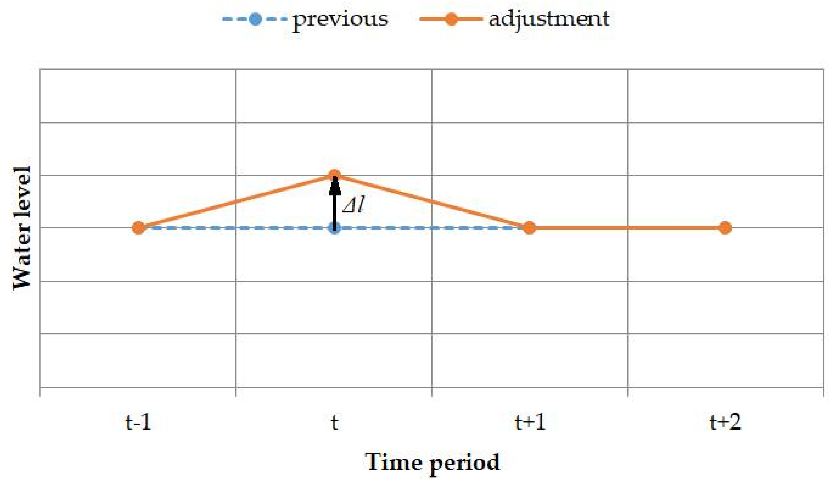
Figure 1. Adjustment in water level by a small gradient.
Algorithms 11 00036 g001
Figure 2. Flowchart of gradient-based search strategy.
Algorithms 11 00036 g002
Figure 3. Flowchart of gradient-based cuckoo search (GCS).
Algorithms 11 00036 g003
Figure 4. Hydrological stations in the Jinsha River.
Algorithms 11 00036 g004
Figure 5. Topology of reservoirs in the Jinsha River.
Algorithms 11 00036 g005
Figure 6. Streamflow of Pingshan station in wet years.
Algorithms 11 00036 g006
Figure 7. Convergence process of the algorithms in the year 1987.
Algorithms 11 00036 g007
Figure 8. The optimal results obtained by GCS in wet years: (a) Wudongde; (b) Baihetan; (c) Xiluodu; and (d) Xiangjiaba.
Algorithms 11 00036 g008aAlgorithms 11 00036 g008b
Figure 9. Streamflow of Pingshan station in normal years.
Algorithms 11 00036 g009
Figure 10. Convergence process of the algorithms in the year 1987.
Algorithms 11 00036 g010
Figure 11. Streamflow of Pingshan station in dry years.
Algorithms 11 00036 g011
Figure 12. Convergence process of the algorithms in year 1977.
Algorithms 11 00036 g012
Table 1. Main parameters of the four cascade hydropower stations in the Jinsha River.
ParametersWudongdeBaihetanXiluoduXiangjiaba
Dead water level (m)945765540370
Normal water level (m)977825600380
Flood limit water level (m)952785560370
Installed capacity (104 kw)102016001260600
Total capacity (108 m3)74.08206.27126.751.63
Minimum outflow (m3/s)90690515001500
Table 2. Test functions.
FunctionFormulaSearch DomainOptimum
Ackley f 1 = 20 exp ( 0.2 1 n i = 1 n x i 2 ) exp ( 1 n i = 1 n cos ( 2 π x i ) ) + e + 20 [−32.768, 32.768] f ( 0 , , 0 ) = 0
Griewank f 2 = 1 + 1 4000 i = 1 n x i 2 i = 1 n cos ( x i i ) [−600, 600] f ( 0 , , 0 ) = 0
Rastrigin f 3 = A n + i = 1 n [ x i 2 A cos ( 2 π x i ) ] [−5.12, 5.12] f ( 0 , , 0 ) = 0
Rosenbrock f 4 = i = 1 n 1 [ 100 ( x i + 1 x i 2 ) 2 + ( x i 1 ) 2 ] [−5, 10] f ( 1 , , 1 ) = 0
Sphere f 5 = i = 1 n x i 2 [−100, 100] f ( 0 , , 0 ) = 0
Bent Cigar f 6 = x 1 2 + 10 6 i = 2 D x i 2 [−100, 100] f ( 0 , , 0 ) = 0
Discus f 7 = 10 6 x 1 2 + i = 2 D x i 2 [−100, 100] f ( 0 , , 0 ) = 0
Happy Cat f 8 = | i = 1 D x i 2 D | 1 / 4 + ( 0.5 i = 1 D x i 2 + i = 1 D x i ) / D + 0.5 [−100, 100] f ( 1 , , 1 ) = 0
Schwefel 2.22 f 9 = i = 1 n | x i | + i = 1 n | x i | [−10, 10] f ( 0 , , 0 ) = 0
Table 3. Errors of test results of the algorithms.
Function IHSKGSACSICS
Shifted AckleyMean4.17 × 10−036.41 × 10−15 *1.16 × 10−027.53 × 10⁻¹⁵
Stdv1.28 × 10−035.54 × 10−151.16 × 10−017.13 × 10⁻¹⁵
Shifted GriewankMean2.34 × 10−021.50 × 10−021.44 × 10−014.04 × 10−05
Stdv3.36 × 10−022.01 × 10−021.32 × 10−011.85 × 10−04
Shifted RastriginMean4.88 × 10−055.894.411.00 × 10−06
Stdv3.03 × 10−053.512.469.84 × 10−06
Shifted RosenbrockMean2.179.88 × 10−012.855.68
Stdv1.761.75 × 10−012.141.70
Shifted SphereMean2.27 × 10−076.88 × 10−322.71 × 10−260.00
Stdv1.41 × 10−075.78 × 10−319.62 × 10−260.00
Shifted Bent CigarMean3.48 × 10+015.76 × 10+026.54 × 10−150.00
Stdv2.50 × 10+018.49 × 10+027.40 × 10−150.00
Shifted DiscusMean1.70 × 10−029.08 × 10+037.25 × 10−150.00
Stdv2.74 × 10−023.27 × 10+037.14 × 10−150.00
Shifted Happy CatMean1.73 × 10−013.61 × 10−023.14 × 10−011.58 × 10−01
Stdv4.17 × 10−021.63 × 10−021.67 × 10−013.67 × 10−02
Shifted Schwefel 2.22Mean2.03 × 10−034.51 × 10−135.48 × 10−131.11 × 10⁻¹⁴
Stdv5.72 × 10−042.35 × 10−122.97 × 10−125.92 × 10⁻¹⁵
Rotated and Shifted SphereMean2.25 × 10−071.63 × 10−018.81 × 10−150.00
Stdv1.59 × 10−079.49 × 10−016.93 × 10−150.00
Rotated and Shifted AckleyMean7.33 × 10−016.66 × 10−152.534.22 × 10−12
Stdv1.036.89 × 10−151.084.21 × 10−11
* PS: The number in bold represent the minimum value.
Table 4. Comparison of power generation (108 kWh) in wet years.
Algorithm1985198719621990
MeanStd.MeanStd.MeanStd.MeanStd.
IHS221627.94215834.23217139.95238240.66
KGSA213512.48206712.4520769.70229212.54
CS225010.7721893.8222145.33242110.34
GCS23220.5222370.0222630.1724840.52
Table 5. Comparison of power generation (108 kWh) in normal years.
Algorithm1997196319701981
MeanStd.MeanStd.MeanStd.Mean Std.
IHS1966284.55210729.492037208.99206535.92
KGSA19538.572021204.31198410.67200710.42
CS20395.24214011.24209612.6020986.48
GCS21050.3822280.4421810.1321590.37
Table 6. Comparison of power generation (108 kWh) in dry years.
Algorithm1973197719841982
MeanStd.Mean Std.MeanStd.Mean Std.
IHS189337.97191333.33 186231.051886 38.38
KGSA18516.9818676.63 18096.631838 6.74
CS19286.0919467.73 18944.481919 4.49
GCS19920.2120190.07 19440.161977 0.17