Damage Identification Algorithm of Hinged Joints for Simply Supported Slab Bridges Based on Modified Hinge Plate Method and Artificial Bee Colony Algorithms

Abstract

Hinge joint damage is a typical form of damage occurring in simply supported slab bridges, which can present adverse effects on the overall force distribution of the structure. However, damage identification methods of hinge joint damage are still limited. In this study, a damage identification algorithm for simply supported hinged-slab bridges based on the modified hinge plate method (MHPM) and artificial bee colony (ABC) algorithms was proposed by considering the effect of hinge damage conditions on the lateral load distribution (LLD) of structures. Firstly, MHPM was proposed and demonstrated, which is based on a traditional hinge plate method by introducing relative displacement as a damage factor to simulate hinge joint damage. The effectiveness of MHPM was verified through comparison with the finite element method (FEM). Secondly, damage identification was treated as the inverse problem of calculating the LLD in damage conditions of simply supported slab bridges. Four ABC algorithms were chosen to solve the problem due to its simple structure, ease of implementation, and robustness. Comparisons of convergence speed and identification accuracy with genetic algorithm and particle swarm optimization were also conducted. Finally, hinged bridges composed of four and seven slabs were studied as numerical examples to account for the feasibility and correctness of the proposed method. The simulation results revealed that the proposed algorithm could identify the location and degree of damaged joints efficiently and precisely.

1. Introduction

Under the influence of vehicle load and natural environmental erosion, structural damages inevitably occur, which can seriously affect the safety and durability of bridges. Therefore, structural damage identification has become an important part of bridge maintenance and reinforcement. Prefabricated reinforced concrete (RC) bridges have become widely used because of their advantages such as higher quality and shorter construction period, etc. As a typical prefabricated RC bridge, most hinged-slab bridges were built decades ago. According to the structural features of a hinged-slab bridge, hinge joints are the relative weak parts, which are prone to cracks (as shown in Figure 1). According to the investigations of more than 500 bridges for expressways in Jilin Province, the maximum proportion of hinge joint damage was 83.3% on the Changchun–Siping Expressway (in operation since 1996) and the minimum was 11.8% for the Jilin–Jiangmifeng Expressway (in operation since 2011). Hinge joint damage in reinforced concrete bridges widely exists, which will cause single slab bearings and aggravate the overall damage status of the structure. Therefore, it is significant to propose an efficient and accurate damage evaluation method for hinge joints for hinged-slab bridges.

In recent decades, structural health monitoring and damage identification, which are based on the dynamic properties of bridges, have been rapidly developed. To measure the dynamic response for structural health monitoring (SHM) accurately and efficiently, Heo et al. [1] developed an intelligent data acquisition system to evaluate the dynamic response performance of bridges using wireless sensor networks in real-time. With the appearance of damage, some changes will take place in modal parameters such as natural frequencies, mode shapes, damping ratios, etc. This feature can be utilized as indicators to identify the location and degree of damage [2,3,4,5]. Researchers also studied damage identification methods based on other identification indicators. For instance, Blachowski et al. [6] proposed a damage localization approach by axial strain accelerations for truss bridges, and Kim et al. [7] developed a damage detection method through Nair’s [7] damage indicator which was demonstrated superior to the modal parameters. Nevertheless, it cannot effectively analyze the damage of transverse connection components for hinged-slab bridges. In addition, hinge joint damage will lead to the redistribution of lateral load, which has an adverse effect on the bearing capacity of bridges. Some researchers have studied the relationship between lateral load distribution (LLD) and the damage condition of hinge joints. Russo et al. [8] performed a series of diagnostic load tests on damaged westbound and undamaged eastbound prestressed concrete bridges to determine the effects of hinge joint damage on load distribution. Test results showed that westbound bridges were somewhat flexible. Change in load distribution occurred when isolated damage was present. Chung et al. [9] investigated the effect of secondary elements and deck cracking on the LLD of girder bridges. Longitudinal cracking was found to increase the load distribution factor up to 17%, while the influence of transverse cracking was not significant. Al-Saidy et al. [10] researched the effect of girder damage on overall load distribution of a typical short-span composite bridge using a grillage method. Kim et al. [11] discovered that live loads were redistributed among the girders due to prestressed CFRP sheets. Azimi et al. [12] studied live load distribution factors of an AASHTO Type 3 precast-prestressed girder, which was calculated through finite element method (FEM) and compared with the simplified method prescribed by other codes. Although great achievements have been obtained in the study of LLD under damage conditions of hinge joints, it is limited in qualitative analysis. If the quantitative relationship for the damage condition of hinge joints with live load distribution can be obtained, damage identification of hinge joints can be achieved.

Therefore, it is essential to calculate the LLD with the damage of lateral connections. Lateral load distribution theory is to convert the spatial live load analysis into planar one, which plays a significant role in bridge design and construction. The main computing methods are determined by the American Association of State Highway Transportation Officials (AASHTO) Standard Specifications and the AASHTO Load and Resistance Factor Design (LRFD) Specification in the United States [13,14], while calculated by the rigid-diaphragm method, hinge plate method, etc. in China [15]. Huo et al. [16] proposed a simplified equal distribution factor method of live load shear which originated from Henry’s [16] method with consideration of the skew angle and span, etc. Wang et al. [17] studied a nine-beam hinged slab bridge which was calculated by comparison with the hinge plate method and the grillage method. Jiao et al. [18] proposed a method based on modal properties for computing the LLD, which was verified by comparison with FEM and the traditional simplified numerical method. The abovementioned methods can accurately calculate the LLD of intact bridge, but it will highlight its limitations for the damaged one. Researchers make a further study on the quantitative relationship of damage conditions and LLD. Wei et al. [19] took into consideration the influence of hinge joints and deck pavement damages and evaluated the LLD with various degrees and locations of damages by the combination of hinge plate method and FEM. Cheng et al. [20] calculated the LLD under different hinge joints damages and used genetic algorithm to identify the damage degree. Jiao et al. [18] utilized the position for cross phenomenon of distribution factor curves between damaged and undamaged bridges as the damage indicator for localizing. The literature demonstrates the great progress in the damage identification of lateral connections, but there is still a great deal of deficiencies. The mentioned methods have their own limitations, for example, it is only suitable for damage identification of a lower degree and it is difficult to guarantee identification accuracy. The purpose of this paper is to establish a modified hinge plate method (MHPM) which can calculate the LLD under arbitrary hinge joint damage conditions.

In practical engineering, it is easy to obtain the LLD of simply supported hinged-slab bridges, which can be equivalently calculated by deflection of the bridge. When parameters such as structural geometries and material properties, etc., are known, the damage identification will be solved by means of MHPM, which can be regarded as an inverse problem of LLD calculation with damages. For such problems, swarm intelligence algorithms including genetic algorithm (GA), particle swarm optimization (PSO), differential evolution (DE), and artificial bee colony algorithm (ABC) present favorable performances [21,22,23,24,25]. For application in practical engineering, Antonelli et al. [26] determined the best configuration of the phase-locked loop system by G.A. Hou et al. [27] who utilized the glowworm swarm optimization algorithm (GSO), which was a new type of PSO, to determine the optimal values of a photovoltaic system, and the results indicated the GSO was obviously superior to traditional algorithms. Among these algorithms, ABC outperforms other algorithms due to its simple structure, easy implementation, and outstanding performance [28,29,30], which have been applied in structural damage identification. Sun et al. [31] presented a modified ABC to identify structural systems, which can realize excellent parameter estimation, even with few measurements and high-noise corruptions. Xu et al. [32] proposed a method for structural damage identification based on Chaotic ABC with residuals of natural frequencies and modal assurance criteria used to establish the objective function. Casciati et al. [25] performed the damage localization of a cable-stayed bridge by comparing both identified and analytical stiffness matrices, and ABC were employed to proceed toward the global minima. The original ABC algorithm was inspired by the cooperative foraging and waggle dance behaviors of honey bee colonies [33]. The ABC has been shown to be competitive with other population-based algorithms. However, there is still an insufficiency in it, which is good at exploration but poor at exploitation [34]. Therefore, different optimization methods are used to enhance the performance of the ABC algorithm [35,36,37,38,39,40,41]. It is worth noting that any improved ABC algorithm is merely suitable for some special numerical optimization problems. In addition, it is necessary to further verify which one is applicable for the damage identification of the hinged-slab bridge.

In this study, an identification algorithm for hinge joint damage of simply supported slab bridges was proposed based on the modified hinge plate method (MHPM) and artificial bee colony (ABC) algorithms. The MHPM was presented by introducing relative displacement as a damage factor to simulate hinge joint damage, which can achieve the acquisition of lateral load distribution for intact and damaged slab bridges. Four kinds of ABC algorithms were used to realize the identification of damage severity of hinge joints, which were compared with GA and PSO. Hinged bridges composed of four and seven slabs and comparisons with the methods in References [19,20] were studied as numerical examples to account for the feasibility and effectiveness of the proposed method.

2. Methods

2.1. Traditional Hinge Plate Method

Slabs at the loading positions deform and other slabs appear to have corresponding deflections, when a hinge slab bridge is subjected to vehicle load. However, the transverse deformation of a single slab is so tiny that it can be negligible. Live load is distributed to every slab because of the internal forces of hinge joints, which include the vertical shear g(x), lateral bending moment m(x), longitudinal shear t(x), and normal force n(x). The height and stiffness of tongue and groove are so weak that other internal forces have little influence compared with vertical shear. Hence, tongue and groove are assumed to be a hinge joint, which only transfer the vertical shear g(x). Meanwhile, the ratio of internal forces, deformations, and distributed loads between slabs should meet the relations expressed in Equation (1):

$$\frac{{\omega }_i\left(x\right)}{{\omega }_j\left(x\right)}=\frac{M_i\left(x\right)}{M_j\left(x\right)}=\frac{Q_i\left(x\right)}{Q_j\left(x\right)}=\frac{P_i\left(x\right)}{P_j\left(x\right)}=constant,$$

(1)

where ω(x), M(x), Q(x), and P(x) are the deflection, bending moment, shear, and distributed load, respectively; i and j represent slab numbers in the range of {1, 2, …, n}, n is the number of slabs.

If the load patterns are concentrated or uniform, relationships of Equation (1) will not be satisfied. Whereas, use of a half-wave sinusoidal load with a peak value p₀, as shown in Figure 2, can harmonize the ratio, which is another assumption for hinge plate method [42].

There are n-1 hinge joints in the bridge composed of n slabs, which means there are n-1 unknown hinge joint forces (namely the vertical shear g(x)). If the whole hinge forces g(x) are solved, the distributed loads on each slab can be obtained according to the principle of balance, which can be used to calculate the influence line vertical value of LLD. According to the location of external load, the calculation form can be divided into two categories. When the external load is located on the side slabs (namely slab 1 or slab n), LLD can be defined by Equations (2) and (3). Equation (4) is used for the case of load placed on internal slabs.

$$\{\begin{array}{ll}{\eta }_{11}=p_{11}=1-g_1\hfill & \\ {\eta }_{i1}=p_{i1}=g_{i-1}-g_i\hfill & \hspace{1em}2\le i\le n-1,\\ {\eta }_{n1}=p_{n1}=g_{n-1}\hfill & \end{array}$$

(2)

$$\{\begin{array}{ll}{\eta }_{1n}=p_{1n}=g_1\hfill & \\ {\eta }_{in}=p_{in}=g_i-g_{i-1}\hfill & \hspace{1em}2\le i\le n-1,\\ {\eta }_{nn}=p_{nn}=1-g_{n-1}\hfill & \end{array}$$

(3)

$$\{\begin{array}{l}{\eta }_{1j}=p_{1j}=g_1\hfill \\ {\eta }_{ij}=p_{ij}=g_i-g_{i-1}\hfill \\ \begin{array}{l}{\eta }_{jj}=p_{jj}=1-g_{j-1}-g_j\\ {\eta }_{kj}=p_{kj}=g_{k-1}-g_k\end{array}\hfill \\ {\eta }_{nj}=p_{nj}=g_n\hfill \end{array}\hspace{1em}\{\begin{array}{l}2\le i\le j-1\hfill \\ j+1\le k\le n-2,\hfill \end{array}$$

(4)

where $p_{ij}$ and ${\eta }_{ij}$ represent the distributed load and LLD influence line vertical value of the ith slab with the external load located at the jth one, respectively; $g_i$ is the vertical shear at ith hinge joint.

For statically indeterminate problem with n − 1 unknown forces, it can be solved by two conditions. One is the basic system (shown in Figure 3) whose hinge joints are cut. Others are the deformation compatibility conditions that the relative vertical displacements of two adjacent slabs at hinge joints are zeros. Therefore, n − 1 canonical equations can be obtained and described as Equation (5):

$$\{\begin{array}{ccccccccccc}{\delta }_{11}{g}_1& +& {\delta }_{12}{g}_2& +& \cdots & +& {\delta }_{1,n-1}{g}_{n-1}& +& {\delta }_{1p}& =& 0\\ {\delta }_{21}{g}_1& +& {\delta }_{22}{g}_2& +& \cdots & +& {\delta }_{2,n-1}{g}_{n-1}& +& {\delta }_{2p}& =& 0\\ ⋮& & ⋮& & \ddots & & ⋮& & ⋮& & ⋮\\ {\delta }_{n-1,1}{g}_1& +& {\delta }_{n-1,2}{g}_2& +& \cdots & +& {\delta }_{n-1,n-1}{g}_{n-1}& +& {\delta }_{n-1,p}& =& 0,\end{array}$$

(5)

where ${\delta }_{ij}$ is the relative vertical displacement at the ith hinge joint when unit sinusoidal joint force is applied in the jth joint; ${\delta }_{ip}$ is the displacement caused by external load p.

Here, an equivalent treatment was conducted that the unit sinusoidal joint force was decomposed into a central force and a sinusoidal torque. It is supposed that ω is the deflection of slab caused by central force and φ is the angle caused by sinusoidal torque. The symbol regulation: when ${\delta }_{ik}$ and $g_i$ are in the same direction, the sign is positive; on the contrary, it is negative. So the deflections of two side slabs are $\omega +\left(b/2\right)\phi$ and $\omega -\left(b/2\right)\phi$, and the overall ${\delta }_{ij}$ and ${\delta }_{ip}$ can be determined through the basic system expressed in Equations (6)–(8):

$$\{\begin{array}{l}{\delta }_{ii}={\omega }_i+\frac{b_i}{2}{\phi }_i+{\omega }_{i+1}+\frac{b_{i+1}}{2}{\phi }_{i+1}\hfill \\ {\delta }_{i,i+1}={\delta }_{i+1,i}=-\left({\omega }_{i+1}-\frac{b_{i+1}}{2}{\phi }_{i+1}\right)\hfill \\ {\delta }_{others}=0\hfill \end{array}\hspace{1em}1\le i\le n-1,$$

(6)

$$\{\begin{array}{ll}{\delta }_{ip}=-{\omega }_i\hfill & \hspace{1em}i=1,n\\ {\delta }_{jp}=0\hfill & \hspace{1em}1\le j\le n\hspace{1em}j\ne i,\end{array}$$

(7)

$$\{\begin{array}{ll}{\delta }_{i-1,p}={\delta }_{ip}=-{\omega }_i\hfill & \hspace{1em}2\le i\le n-1\\ {\delta }_{jp}=0\hfill & \hspace{1em}1\le j\le n\hspace{1em}j\ne i\ne i-1,\end{array}$$

(8)

where ${\omega }_i\left(x\right)=\frac{p{l}^4}{{\pi }^4{E}_i{I}_i}\sin \frac{\pi x}{l}$, ${\phi }_i\left(x\right)=\frac{p{b}_i{l}^2}{2{\pi }^2{G}_i{I}_{Ti}}\sin \frac{\pi x}{l}$; l is the span of the hinge slab bridge; $b_i$, $E_i$, $G_i$, $I_i$ and $I_{Ti}$ represent the cross section width, elastic modulus, shear modulus, bending moment of inertia and torsional moment of inertia of the ith slab, respectively.

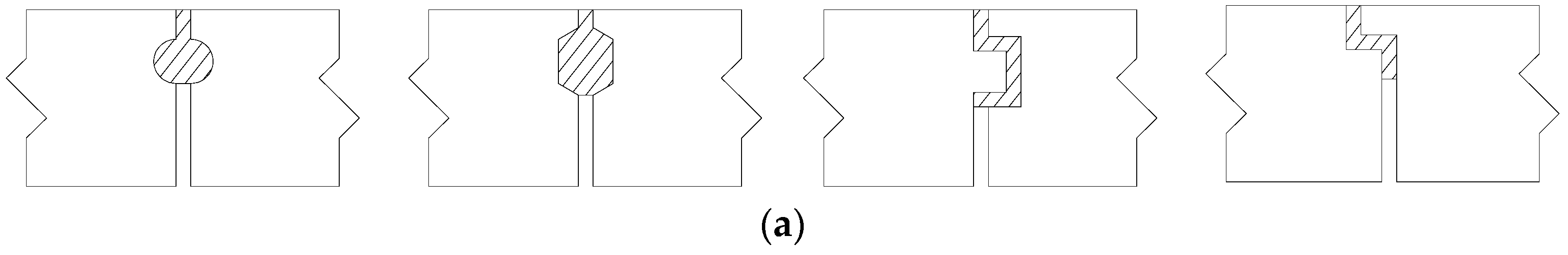
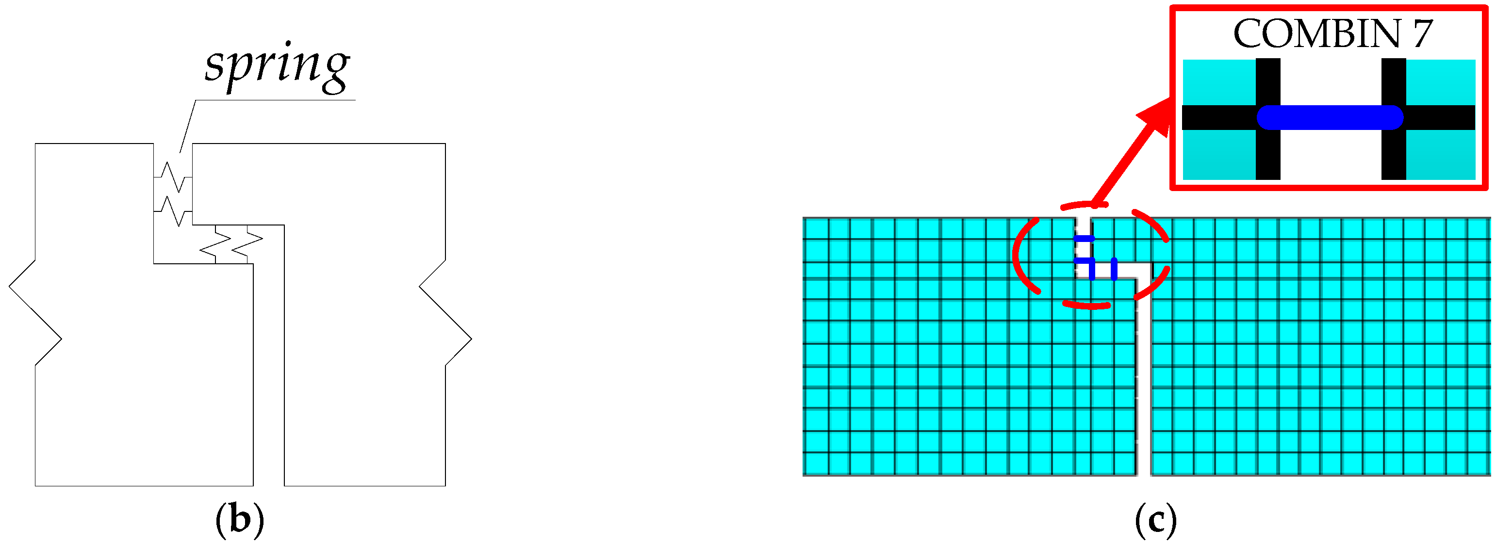
2.2. Modified Hinge Plate Method

The strength of hinge joint is weaker than other parts of the bridge, which will be damaged firstly. Consequently, there must be some changes in vertical shear transfer by the hinges. Right-side value of canonical equation represents the relative displacement of two adjacent slabs at the hinge, which is zero for the intact bridge. When the hinge joint damage occurs, the relative displacement can be regarded as damage indicator (shown in Figure 4), which is nonzero and proportional to the degree of damage. μ is the degree of damage in the range of [0, 1]. For the general case, the indicator can be expressed as Equation (9):

$$\mathsf{\Delta }={\mu }_i\times ({\delta }_{ip}+{\delta }_{i,j}\times g_j),$$

(9)

where ${\mu }_i$ is the damage factor of the ith hinge joint; ${\delta }_{ip}$, ${\delta }_{i,j}$ and $g_j$ have the same meanings with that of Equation (5) except the subscript j, which represents the hinge number closed to the ith joint at the side of external load.

If μ equals 1, it demonstrates the hinge is damaged, which cannot transfer the distributed load any more. At this condition, the displacement is described as $\mathsf{\Delta }=1\times ({\delta }_{ip}+{\delta }_{i,j}\times g_j)$. It should be noticed that the displacement of No. 1 joint will be expressed as $\mathsf{\Delta }={\mu }_1\times {\delta }_{1p}$ when the load is located on No. 1 slab. The principle is the same with No. (n − 1) joint when the load is placed on the side slab No. n.

Here, we assume the hinge joint damage case is $[{\mu }_1,{\mu }_2,\cdots ,{\mu }_{n-1}]$, which depicts the damage degrees for the whole hinge joints. When the external load is placed on slab 1, slab i (the arbitrary internal slab) and slab n, the canonical equations will be redefined as Equations (10)–(12).

Table 1. Pseudo-code of modified hinged plate method.

Algorithm: The load lateral distribution influence line
Input: the number of slabs: n; Young’s modulus vector: E; the slab number to be calculated: SN
the three-dimensional geometry parameter of slab: l, b, h; the damage condition of hinged joints: μ
01	Calculate ${\omega }_i$ and ${\phi }_i$ through the illustration of Equation (8)
02	for FP = 1: n
03	switch FP
04	case 1
05	Calculate δij and δip by Equations (6) and (7), respectively
06	Calculate the relative displacement through the right side of Equation (10)
07	Solve Equation (10) and obtain g = [g1, …, gi, …, gn−1]
08	Calculate the load lateral distribution vertical value by Equation (2)
09	case n
10	Calculate δij and δip by Equations (6) and (7), respectively
11	Calculate the relative displacement through the right side of Equation (12)
12	Solve Equation (12) and obtain g = [g1, …, gi, …, gn−1]
13	Calculate the load lateral distribution vertical value by Equation (3)
14	otherwise
15	Calculate δij and δip by Equations (6) and (8), respectively
16	Calculate the relative displacement through the right side of Equation (11)
17	Solve Equation (11) and obtain g = [g1, …, gi, …, gn−1]
18	Calculate the lateral load distribution vertical value by Equation (4)
19	end switch
20	Memory the objective lateral load distribution vertical value ${\eta }_{SN,FP}$
21	end for
Output: The load lateral distribution influence line of Slab SN: $[{\eta }_{SN,1},\cdots ,{\eta }_{SN,i},\cdots ,{\eta }_{SN,n}]$

shows the calculation flow for LLD of the hinged-slab bridge under damage conditions.

$$\{\begin{array}{lllllllllll}{\delta }_{1,1}{g}_1& +& {\delta }_{1,2}{g}_2& +& \cdots & +& {\delta }_{1,n-1}{g}_{n-1}& +& {\delta }_{1,p}& =& {\mu }_1{\delta }_{1,p}\\ ⋮& & ⋮& & \ddots & & ⋮& & ⋮& & ⋮\\ {\delta }_{i-1,1}{g}_1& +& {\delta }_{i-1,2}{g}_2& +& \cdots & +& {\delta }_{i-1,n-1}{g}_{n-1}& +& {\delta }_{i-1,p}& =& {\mu }_{i-1}\left({\delta }_{i-1,p}+{\delta }_{i-1,i-2}{g}_{i-2}\right)\\ {\delta }_{i,1}{g}_1& +& {\delta }_{i,2}{g}_2& +& \cdots & +& {\delta }_{i,n-1}{g}_{n-1}& +& {\delta }_{i,p}& =& {\mu }_i\left({\delta }_{i,p}+{\delta }_{i,i-1}{g}_{i-1}\right)\\ ⋮& & ⋮& & \ddots & & ⋮& & ⋮& & ⋮\\ {\delta }_{n-1,1}{g}_1& +& {\delta }_{n-1,2}{g}_2& +& \cdots & +& {\delta }_{n-1,n-1}{g}_{n-1}& +& {\delta }_{n-1,p}& =& {\mu }_{n-1}\left({\delta }_{n-1,p}+{\delta }_{n-1,n-2}{g}_{n-2}\right),\end{array}$$

(10)

$$\{\begin{array}{lllllllllll}{\delta }_{1,1}{g}_1& +& {\delta }_{1,2}{g}_2& +& \cdots & +& {\delta }_{1,n-1}{g}_{n-1}& +& {\delta }_{1,p}& =& {\mu }_1\left({\delta }_{1,p}+{\delta }_{1,2}{g}_2\right)\\ ⋮& & ⋮& & \ddots & & ⋮& & ⋮& & ⋮\\ {\delta }_{i-1,1}{g}_1& +& {\delta }_{i-1,2}{g}_2& +& \cdots & +& {\delta }_{i-1,n-1}{g}_{n-1}& +& {\delta }_{i-1,p}& =& {\mu }_{i-1}\left({\delta }_{i-1,p}+{\delta }_{i-1,i}{g}_i\right)\\ {\delta }_{i,1}{g}_1& +& {\delta }_{i,2}{g}_2& +& \cdots & +& {\delta }_{i,n-1}{g}_{n-1}& +& {\delta }_{i,p}& =& {\mu }_i\left({\delta }_{i,p}+{\delta }_{i,i-1}{g}_{i-1}\right)\\ ⋮& & ⋮& & \ddots & & ⋮& & ⋮& & ⋮\\ {\delta }_{n-1,1}{g}_1& +& {\delta }_{n-1,2}{g}_2& +& \cdots & +& {\delta }_{n-1,n-1}{g}_{n-1}& +& {\delta }_{n-1,p}& =& {\mu }_{n-1}\left({\delta }_{n-1,p}+{\delta }_{n-1,n-2}{g}_{n-2}\right),\end{array}$$

(11)

$$\{\begin{array}{lllllllllll}{\delta }_{1,1}{g}_1& +& {\delta }_{1,2}{g}_2& +& \cdots & +& {\delta }_{1,n-1}{g}_{n-1}& +& {\delta }_{1,p}& =& {\mu }_1\left({\delta }_{1,p}+{\delta }_{1,2}{g}_2\right)\\ ⋮& & ⋮& & \ddots & & ⋮& & ⋮& & ⋮\\ {\delta }_{i-1,1}{g}_1& +& {\delta }_{i-1,2}{g}_2& +& \cdots & +& {\delta }_{i-1,n-1}{g}_{n-1}& +& {\delta }_{i-1,p}& =& {\mu }_{i-1}\left({\delta }_{i-1,p}+{\delta }_{i-1,i}{g}_i\right)\\ {\delta }_{i,1}{g}_1& +& {\delta }_{i,2}{g}_2& +& \cdots & +& {\delta }_{i,n-1}{g}_{n-1}& +& {\delta }_{i,p}& =& {\mu }_i\left({\delta }_{i,p}+{\delta }_{i,i+1}{g}_{i+1}\right)\\ ⋮& & ⋮& & \ddots & & ⋮& & ⋮& & ⋮\\ {\delta }_{n-1,1}{g}_1& +& {\delta }_{n-1,2}{g}_2& +& \cdots & +& {\delta }_{n-1,n-1}{g}_{n-1}& +& {\delta }_{n-1,p}& =& {\mu }_{n-1}{\delta }_{n-1,p}.\end{array}$$

(12)

2.3. Artificial Bee Colony (ABC) Algorithm

2.3.1. Original ABC Algorithm

With the aim to solve numerical function optimization, the original ABC, which was designed by Karaboga [33] in 2005, is a modern heuristic algorithm inspired by the cooperative foraging and waggle dance behaviors of honey bee colonies. Solutions are called food sources in ABC, which are explored by employed bees, and the best solutions are stored in their memories. Since each food source is possessed by a unique employed bee, the numbers of employed bees or onlooker bees equals the number of food source positions (solutions). According to the functions of artificial bees in ABC, they can be divided into three categories, namely employed bees, onlooker bees, and scout bees. Correspondingly, the ABC algorithm is composed of four phases, such as the initialization phase, employed bees phase, onlooker bees phase, and scout bees phase.

(1) Initialization phase

At first, basic parameters are initialized, which include the number of food source (BN), the termination criteria (maximum number of iterations and error goal), and the control parameter limit. The dimension D of a solution is equal to the number of hinge joints in this paper. Then, an initial food source (solution) is generated by Equation (13) and the fitness, described as Equation (14), is used to evaluate the quality of the food source.

$$x_{ij}=l{b}_j+(u{b}_j-l{b}_j)\cdot rand(0,1),$$

(13)

where $x_{ij}$ is the jth parameter of the ith solution, $i=1,2,\dots ,BN$, $j=1,2,\dots ,D$; $l{b}_j$ and $u{b}_j$ are the lower and upper bounds of the jth parameter respectively; $rand(0,1)$ is a uniform distributed real number in the interval between 0 and 1.

$$fi{t}_i=\{\begin{array}{c}\frac{1}{1+f(x_i)}\\ 1+abs(f(x_i))\end{array}\begin{array}{c}iff(x_i)\ge 0\\ otherwise\end{array},$$

(14)

where $fi{t}_i$ represents the fitness of the ith solution; $f(x_i)$ is the objective function value of the food solution $x_i$.

(2) Employed bees phase

Artificial employed bees will search the vicinity of its own food source. A new random solution will be found and the better one between two solutions can be reserved according to the greedy selection mechanism. This process is defined as Equation (15):

$$v_{ij}=x_{ij}+{\psi }_{ij}\cdot (x_{ij}-x_{kj}),$$

(15)

where $v_{ij}$ is the jth parameter of the ith new solution; $x_{kj}$ is a food source selected randomly in the swarm, and k is not equal to i; ${\psi }_{ij}$ is a random number in the range of [−1, 1].

(3) Onlooker bees phase

After employed bees search the food sources, onlooker bees will obtain the nectar information and choose a food source (solution) by its probability $p_i$, which is calculated by Equation (16). In other words, the higher fitness of the food source is, the more onlooker bees will select it to exploit further. The greedy selection mechanism is implemented again to memory the best solution so far.

$$p_i=\frac{fi{t}_i}{{\displaystyle \sum _{j=1}^{BN}fi{t}_j}}.$$

(16)

(4) Scout bee phase

In this phase, if the counter value of a food source exceeds the control parameter limit, the employed bee will turn to be a scout bee by Equation (13). After obtaining the new food source, the scout bee converts back into an employed bee and the counter is reset to zero. The steps from (2) to (4) will be repeated until one of the termination criteria is met, namely, the error of the solution is lower than the error goal or the number of cycles reaches the maximum number of iteration.

2.3.2. Improved ABC Algorithms

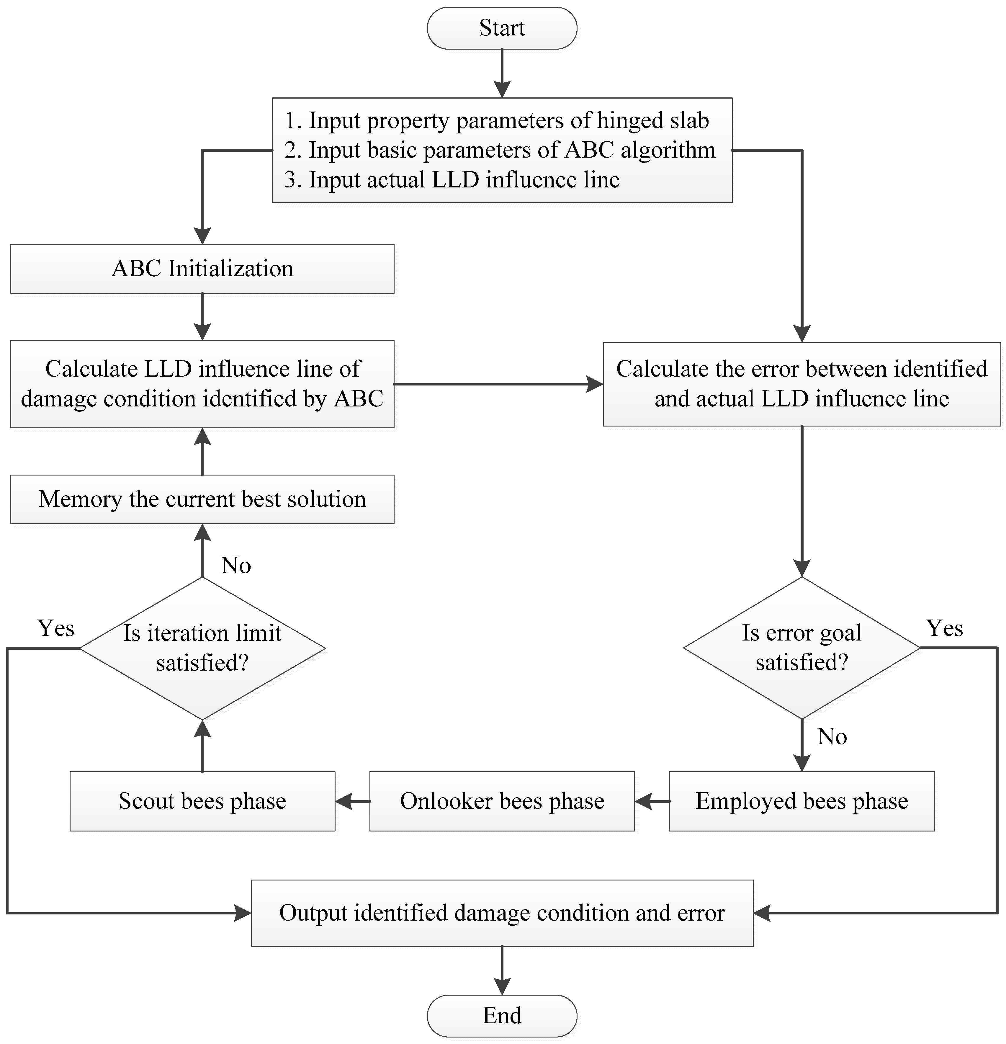
In more than a decade, great achievements have been obtained in the optimization of the ABC algorithm. The ABCG proposed by Xiang et al. [39], ABCLGII developed by Lin et al. [40], and HABCDE defined by Jadon et al. [41] have been proven to possess more favorable performance than other improved ABC algorithms in aspects of calculation accuracy, robustness, and convergence rate. Therefore, the original ABC and three improved algorithms (ABCG, ABCLGII, and HABCDE) are selected as the damage identification algorithms to estimate which one is the most suitable for the proposed strategy in this study. The specific parameters of ABCG, ABCLGII, and HABCDE shown in

Table 2. Optimization parameters values.

Algorithms	The Parameter Values
ABCG 1	$G=0.1$; $\epsilon =2^{-52}$; $\alpha =0.95$; $\beta =0.15$; $\delta =0.95$; $\xi =0.98$
ABCLGII 2	$r=2$; $q=0.2$; $P_{str}=0.5$
HABCDE 3	$C=1$; $CR=0.6$; $F=0.5$

¹ An improved artificial bee colony algorithm based on the gravity model; ² A novel artificial bee colony algorithm with local and global information interaction; ³ A hybrid artificial bee colony with differential evolution.

can be seen in the literature [39,40,41].

2.4. Methodology

The basic algorithms for the hinge damage identification algorithm have been described in detail. In conclusion, the overall steps of the proposed algorithm are presented as follows:

• Firstly, each slab deflection of hinged bridges are measured through a static experiment with external loads and the corresponding parameters of the bridge should be obtained;
• Secondly, the actual LLD influence line can be calculated by the deflections in the first step;
• Thirdly, we can generate an ABC model, of which the objective function is the Euclidean distance between the actual LLD influence line and the one calculated by the MHPM method;
• Lastly, we can search the solution with the best fitness by original or improved ABC algorithm, and the best solution is the identified hinge joint damage degree and location of the hinged-slab bridge.

3. Results and Discussion

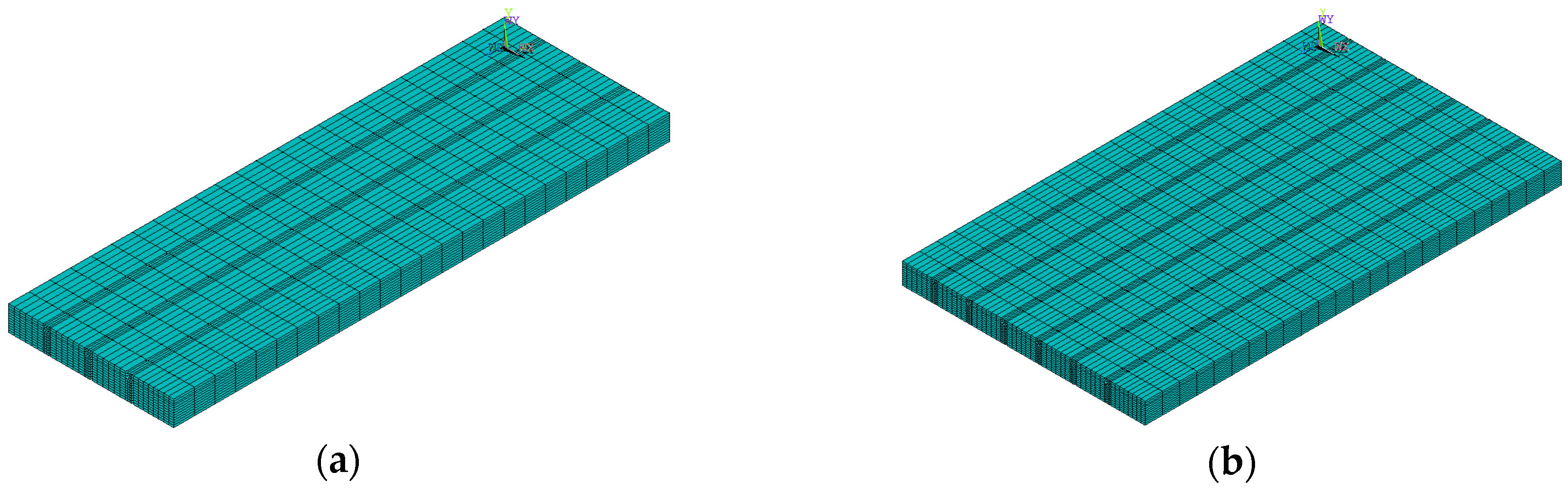
3.1. Lateral Load Distribution Evaluation Based on Modified Hinge Plate Method

Simply supported slab bridges composed of four and seven slabs were selected as the research objects in this study, whose cross-section form of a single slab was rectangular. The sizes of width and height were 1 m and 0.6 m, respectively. The span of the bridge was 12 m, and the material properties of elements were elastic modulus E = 3.5 × 10¹⁰ Pa, Poisson’s ratio μ = 0.2, density ρ = 2500 kg/m³. The finite element model was established by ANSYS 14.0 and composed through SOLID 65 element. A general hinge joint mode is shown in Figure 5a. For the convenience of analysis, the hinge joint was simplified as shown Figure 5b. The spring element COMBIN 7 was selected to simulate the damage through reduction of spring stiffness, which is depicted in Figure 5c. Here, an undamaged hinge joint was considered to have infinite stiffness, while the spring stiffness with damage extent ${\mu }_i$ could be calculated by Equation (17). It should be noted that all numerical computations and algorithm programs were implemented in MATLAB 2014b and run on a Core i5-6500 personal computer with Windows 7 system, 3.20 GHz CPU and 8 GB RAM Memory.

$$k_i=\frac{g_i}{{\mu }_i\left({\delta }_{i,p}+{\delta }_{i,j}{g}_j\right)}\times 0.5,$$

(17)

where k_i is the spring stiffness.

The deflections of each slab at mid-span cross section can be calculated based on finite element simulation. According to the statics calculating procedure of LLD, it can be obtained by:

$${\eta }_{ki}=\frac{{\omega }_{ki}}{{\displaystyle \sum _{j=1}^n{\omega }_{ji}}},$$

(18)

where ${\omega }_{ki}$ is deflection of the kth slab at mid-span cross-section when the external load is located at mid-span of the ith slab.

The efficiency and accuracy of MHPM were verified by comparing its results with those calculated through FEM. Damage cases of hinge joints for simply supported bridges with four and seven slabs (as shown in Figure 6) are listed in

Table 3. Hinge joint damage cases for simply supported bridge with four slabs.

Case No.	Damage Location and Extent	Slab Nos. for LLD 1
1	[0.18, 0, 0]	1, 3
2	[0, 0.33, 0]	2, 4
3	[0.05, 0.15, 0]	2, 3
4	[0.22, 0.10, 0.43]	1, 2

¹ Lateral load distribution.

and

Table 4. Hinge joint damage cases for simply supported bridge with 7 slabs.

Case No.	Damage Location and Extent	Slab Nos. for LLD
5	[0.05, 0, 0, 0, 0, 0]	1, 4
6	[0, 0, 0.6, 0, 0, 0]	2, 5
7	[0.1, 0, 0, 0.5, 0, 0]	1, 3
8	[0.1, 0.15, 0, 0.4, 0.05, 0]	4, 7

, respectively. Corresponding LLD influence lines of overall cases were shown in Figure 7 and Figure 8. In the figures, MHPM and FEM represent two methods, while D and U mean the hinge joint was damaged and undamaged, respectively.

As can be seen from Figure 7 and Figure 8, LLD influence lines computed by MHPM were consistent with the results obtained through FEM. Compared with FEM, which was taken as the benchmark method, the relative error of LLD for a single slab calculated by MHPM did not exceed 1.9%. It demonstrates the correctness of MHPM proposed in this paper. In the case of single hinge joint damage, namely cases 1, 2, 5, and 6, cross phenomena of LLD influence lines between damaged and undamaged cases coincided with results found in the literature [18]. With respect to the multiple damaged location cases (cases 3, 4, 7, 8), in which there was still one cross point, multiple damaged hinge joints cannot be identified through the cross phenomena merely. How to identify the damage degree and location quantitatively needs to be investigated furtherly.

To evaluate the effects of hinge joint damage degree on the LLD of simply supported slab bridges, different damage conditions of hinge joints were discussed. Lateral load distribution for simply supported bridge with four and seven slabs under single and multiple hinge joint damage conditions are illustrated in Figure 9 and Figure 10, respectively. It can be found from the results that the offset degrees of LLDs for damaged bridges are proportional to damage degrees. The greater the damage degrees are, the more severe the distortions are present. It indicates that the offset rate of LLD can realize the qualitive assessment of hinge joint damage.

3.2. Damage Severity Identification of Hinge Joint Based on Artificial Bee Colony

3.2.1. Damage Identification Process

Damage identification is formulated as an optimization problem in the ABC algorithm. By this way, Euclidean distance between the actual measured LLD influence line and the result calculated by MHPM is defined as the objective function, which is expressed in Equation (19). Meanwhile, the function can be used to evaluate the error of damage identification. The smaller the objective function value is, the more precise the damage identification result is. In consequence, the error goal was set to be 10⁻²⁰. If the error of damage identification result was less than the error goal, the algorithm will be terminated immediately; otherwise, it runs until the maximum number of iterations. To be specific, the flowchart of damage identification for a hinged-slab bridge is shown in Figure 11.

$$f=\sqrt{{\displaystyle \sum _{i=1}^n{({\eta }_{i,jI}-{\eta }_{i,jA})}^2}},$$

(19)

where ${\eta }_{i,jI}$ and ${\eta }_{i,jA}$ represent the identified and actual ith vertical value of LLD influence line of slab j, respectively.

In ABC, ABCG, ABCLGII, and HABCDE algorithms, basic parameters are chosen to be the same, so that a fair comparison can be made. Damage identification accuracy will be improved with the increase of bee colony size, but it will also greatly increase the time cost of the calculation process [28,29]. According to the literature [21,33,34,35], the bee colony size BN, which is equal to the number of food sources, is set to be 50 in all calculations. The control parameter limit is limit = BN × D [29], where D is introduced in Section 3.1. And the maximum number of iterations is set to be 500. As for the parameters of GA and PSO, the crossover and mutation probabilities of GA are 0.7 and 0.05. The inertia weight and two acceleration coefficients in PSO are 0.5, 1.5, and 2.5, respectively. The specific theory and process of GA and PSO can be seen in References [43,44].

3.2.2. Numerical Simulations

For damage severity assessment of hinge joint damage in simply supported bridges with four slabs, LLD influence lines for damage cases listed in Table 3 were first obtained and listed in

Table 5. LLD influence lines for damage cases listed in Table 3.

Case No.	Slab No.	LLD Influence Line Vertical Value
		1	2	3	4
1	1	0.41844	0.19806	0.17576	0.16496
	3	0.18972	0.26694	0.27956	0.27774
2	2	0.35677	0.36376	0.14416	0.13531
	4	0.12700	0.13531	0.35677	0.38093
3	2	0.29225	0.32085	0.20157	0.18919
	3	0.17522	0.20219	0.31539	0.31137
4	1	0.49264	0.23551	0.17375	0.07614
	2	0.25219	0.37177	0.28635	0.12548

. Iteration processes for damage identification using ABC algorithms, GA, and PSO were illustrated in Figure 12. Corresponding identification results and time costs are listed in

Table 6. Damage identification results for cases 1 to 4.

Case No.	Slab No.	Algorithms	Hinge Joint No.
			1	2	3
1	1	ABC	0.18	5.643 × 10−10	0
		ABCG	0.18	5.646 × 10−10	0
		ABCLGII	0.18	5.641 × 10−10	0
		HABCDE	0.18	0	0
		GA	0.1802	7.630 × 10−6	4.252 × 10−9
		PSO	0.18	0	0
	3	ABC	0.18	3.512 × 10−10	1.724 × 10−9
		ABCG	0.18	3.504 × 10−10	1.725 × 10−9
		ABCLGII	0.18	3.505 × 10−10	1.725 × 10−9
		HABCDE	0.18	3.506 × 10−10	1.725 × 10−9
		GA	0.1799	3.064 × 10−5	1.526 × 10−5
		PSO	0.18	0	0
2	2	ABC	4.140 × 10−10	0.33	0
		ABCG	4.142 × 10−10	0.33	0
		ABCLGII	4.139 × 10−10	0.33	0
		HABCDE	4.141 × 10−10	0.33	0
		GA	2.998 × 10−8	0.33	6.199 × 10−6
		PSO	0	0.33	0
	4	ABC	1.753 × 10−9	0.33	0
		ABCG	1.753 × 10−9	0.33	0
		ABCLGII	1.753 × 10−9	0.33	1.998 × 10−15
		HABCDE	1.754 × 10−9	0.33	2.998 × 10−15
		GA	0	0.3457	0
		PSO	0	0.33	0
3	2	ABC	0.05	0.15	0
		ABCG	0.05	0.15	0
		ABCLGII	0.05	0.15	0
		HABCDE	0.05	0.15	0
		GA	0.0489	0.1485	0.0039
		PSO	0	0.1377	0
	3	ABC	0.05	0.15	0
		ABCG	0.0499	0.15	0
		ABCLGII	0.05	0.15	0
		HABCDE	0.05	0.15	0
		GA	0.0547	0.1484	0
		PSO	0	0.159	0
4	1	ABC	0.22	0.1	0.43
		ABCG	0.22	0.1	0.43
		ABCLGII	0.22	0.1	0.43
		HABCDE	0.22	0.1	0.43
		GA	0.2166	0.1261	0.501
		PSO	0.22	0.1	0.43
	2	ABC	0.22	0.1	0.43
		ABCG	0.22	0.1	0.43
		ABCLGII	0.22	0.1	0.43
		HABCDE	0.22	0.1	0.43
		GA	0.1953	0.0525	0.5378
		PSO	0.22	0.1	0.43

and

Table 7. Time costs for cases 1 to 4 (unit: s).

Case No.		1		2		3		4
Slab No.		1	3	2	4	2	3	1	2
Algorithms	ABC	432	429	434	435	449	454	476	471
	ABCG	435	430	432	431	453	451	475	473
	ABCLGII	53	49	51	54	52	51	54	56
	HABCDE	56	55	57	56	59	63	62	65
	GA	23	22	19	21	25	23	28	29
	PSO	20	21	20	22	21	22	26	24

.

As can be seen from the results, ABC, ABCG, ABCLGII, and HABCDE presented favorable identification accuracies for all damage cases of hinge joints. Particle swarm optimization also possessed good precision except in case 3 (multiple damages for joints 1 and 2). The relative errors for slabs 2 and 3 in case 3 were 8.2% and 6.0%, respectively. The GA presented the worst identification results among these methods. As for calculation speed, PSO possessed the lowest time cost. Among the ABC algorithms, ABCLGII presented the most favorable efficiency.

A simply supported hinged-slab bridge composed of seven slabs was also adopted as the numerical analysis example. Under the damage cases of Table 4, the LLD influence lines calculated by MHPM were shown in

Table 8. LLD influence lines for damage cases listed in Table 4.

Case No.	Slab No.	LLD Influence Line Vertical Value
		1	2	3	4	5	6	7
5	1	0.26629	0.18381	0.14782	0.12150	0.10314	0.09153	0.08590
	4	0.11814	0.13872	0.15553	0.16616	0.15493	0.13749	0.12904
6	2	0.29513	0.29808	0.28782	0.03595	0.03052	0.02708	0.02542
	5	0.02767	0.02948	0.03322	0.23341	0.23824	0.22593	0.21205
7	1	0.34244	0.21413	0.18510	0.16820	0.03313	0.02940	0.02760
	3	0.17655	0.22862	0.23877	0.23183	0.04567	0.04053	0.03804
8	4	0.12022	0.15568	0.25309	0.27135	0.07970	0.06187	0.05807
	7	0.02463	0.03190	0.05186	0.05895	0.22806	0.28812	0.31649

. After the damage identification calculated by the proposed method, the iteration process and damage condition results based on ABC algorithms, GA, and PSO are described in Figure 13 and

Table 9. Damage identification results for case 5 to case 8.

Case No.	Slab No.	Algorithms	Hinge Joint No.
			1	2	3	4	5	6
5	1	ABC	0.05	0	0	0	0	0
		ABCG	0.05	5.740 × 10−10	0	0	0	0
		ABCLGII	0.05	5.275 × 10−10	0	0	0	3.035 × 10−9
		HABCDE	0.05	5.597 × 10−10	0	0	1.786 × 10−10	0
		GA	0.0625	0	0	0	0	0
		PSO	0.05	0	0	0	0	0
	4	ABC	0.0500001	0	0	0	0	0
		ABCG	0.05	0	0	0	0	0
		ABCLGII	0.05	1.384 × 10−9	0	1.050 × 10−9	1.486 × 10−10	3.510 × 10−10
		HABCDE	0.05	1.386 × 10−9	0	1.049 × 10−9	2.280 × 10−10	0
		GA	0.0626	0	0	0	4.768 × 10−7	0
		PSO	0.05	0	0	0	0	0
6	2	ABC	0	0	0.6	0	0	0
		ABCG	0	0	0.6	2.644 × 10−9	0	0
		ABCLGII	0	0	0.6	2.640 × 10−9	0	0
		HABCDE	0	0	0.6	2.644 × 10−9	0	0
		GA	0	6.820 × 10−13	0.6441	2.980 × 10−8	0	7.629 × 10−6
		PSO	0	0	0.6	0	0	0
	5	ABC	0	0	0.6	0	0	2.514 × 10−10
		ABCG	0	0	0.6	0	0	0
		ABCLGII	2.598 × 10−14	0	0.6	5.820 × 10−10	5.523 × 10−10	2.002 × 10−10
		HABCDE	9.992 × 10−15	0	0.6	5.828 × 10−10	5.534 × 10−10	1.996 × 10−10
		GA	3.074 × 10−8	0	0.5977	3.243 × 10−5	2.235 × 10−8	1.073 × 10−6
		PSO	0	0	0.6	0	0	0
7	1	ABC	0.1	6.030 × 10−9	0	0.5	0	3.176 × 10−9
		ABCG	0.1	0	0	0.5	0	0
		ABCLGII	0.1	2.428 × 10−10	0	0.5	0	2.998 × 10−15
		HABCDE	0.1	2.423 × 10−10	0	0.5	0	0
		GA	0.1250	0	0	0.5002	1.513 × 10−8	0
		PSO	0.1	0	0	0.5	0	0
	3	ABC	0.1	0	0	0.5	0	0
		ABCG	0.1	0	0	0.5	0	0
		ABCLGII	0.1	3.608 × 10−10	7.175 × 10−10	0.5	0	0
		HABCDE	0.1	3.612 × 10−10	7.182 × 10−10	0.5	0	0
		GA	0.1250	4.888 × 10−6	2.328 × 10−10	0.5010	2.384 × 10−7	1.197 × 10−7
		PSO	0.1	0	0	0.5	0	0
8	4	ABC	0.0999	0.150002	0	0.400001	0.0499	2.300 × 10−6
		ABCG	0.1	0.15	0	0.4	0.05	0
		ABCLGII	0.1	0.15	0	0.4	0.05	0
		HABCDE	0.1	0.15	0	0.4	0.05	0
		GA	0.0625	0.1885	0	0.4119	1.967 × 10−6	0
		PSO	0.1012	0.1505	0	0.4093	0	0
	7	ABC	0.1	0.1499	0	0.4	0.0499	0
		ABCG	0.1001	0.1499	0	0.400004	0.050001	0
		ABCLGII	0.1	0.15	0	0.4	0.05	6.652 × 10−10
		HABCDE	0.1	0.15	0	0.4	0.05	6.656 × 10−10
		GA	0.0674	0.1765	0	0.3988	0.0449	0.0019
		PSO	0.2218	0	0.0397	0.4287	0	0

and

Table 10. Time cost for case 5 to case 8 (unit: s).

Case No.		5		6		7		8
Slab No.		1	4	2	5	1	3	4	7
Algorithms	ABC	641	655	631	647	753	701	768	787
	ABCG	660	673	666	628	740	724	747	753
	ABCLGII	59	53	59	61	58	58	60	62
	HABCDE	60	60	62	61	64	66	69	69
	GA	23	25	20	24	23	24	28	27
	PSO	22	23	22	25	24	25	29	28

.

As shown in Figure 13, damage identification based on ABCLGII had the fastest convergence rate among the ABC algorithms. It could converge after 100 iterations from case 1 to case 3, while the convergence rate decreased to 180 cycles for case 4, which is a more complicated damage condition. The HABCDE algorithm ranked only second to the ABCLGII in terms of convergence rate. With the complexity of damage conditions increased, its convergence rate decreased from 200 to 400 iterations. As for the other two algorithms, the convergence rate of ABCG was unstable. The original ABC algorithm had the worst performance, which converged after almost 500 iterations in all damage cases. In the aspect of calculation error, the three improved ABC algorithms had similar performances, of which the error was approximately 5 × 10⁻¹⁰. But in the last case, ABCG had a maximum error of 4.72 × 10⁻⁶. The original ABC algorithm error fluctuated within a range of 1.79 × 10⁻⁹ and 9.68 × 10⁻⁷. The time cost of the damage identification algorithm based on ABCLGII and HABCDE did not exceed 70 s for 500 iterations, while that of the others needed 10 to 15 min.

As can be seen from Table 9, the relative error of a single hinge joint damage level was no more than 2 × 10⁻⁵, while those of case 1 to case 3 were much less than this value. It demonstrates that the damage identification method based on MHPM and original or improved ABC algorithms can successfully identify the location and degree of hinge joint damage, which has favorable applicability and accuracy. Taking into consideration the convergence rate, identification accuracy, and time cost, the ABCLGII algorithm is more suitable for the damage identification method proposed in this paper.

Comparations with PSO and GA were also conducted. Particle swarm optimization presented favorable convergence speed and identification accuracy for most of the damage cases except case 4 (multiple damages for joints 1, 2, 4, and 5). In this case, the identification results of PSO were unacceptable. As for GA, it presented the most unsatisfactory results among these methods.

In order to verify the applicability of the proposed damage identification method in this article, we compared the damage identification results for several cases of Table 3 and Table 4 (as shown in

Table 11. Hinge joint damage identification results comparison.

Case No.	Slab No.	Algorithms	Damage Identification Results	Error
2	2	In this article	[4.139 × 10−10, 0.33, 0]	0
		[19]	[0.04, 0.41, 0]	0.079
		[20]	[0, 0.38, 0.03]	0.063
3	3	In this article	[0.05, 0.15, 0]	0
		[19]	[0.033, 0.14, 0]	0.017
		[20]	[0.046, 0.155, 0]	0.014
5	1	In this article	[0.05, 5.275 × 10−10, 0, 0, 0, 3.035 × 10−9]	0
		[19]	[0.057, 0, 0, 0, 0, 0]	0.005
		[20]	[0.048, 0, 0, 0, 0, 0]	0.003
7	3	In this article	[0.1, 3.608 × 10−10, 7.175 × 10−10, 0.5, 0, 0]	0
		[19]	[0.15, 0.03, 0.12, 0.41, 0.07, 0]	0.164
		[20]	[0.13, 0, 0.09, 0.54, 0.049, 0]	0.118

), which were calculated by the algorithms in this article and References [19,20], respectively. The error in Table 11 was computed by Equation (19).

As can be seen from Table 11, the proposed algorithm in this paper has zero error, which means it has the best performance for damage identification. Although some undamaged hinge joints were identified as damage through the method of this paper; the identified damage was less than 3.035 × 10⁻⁹ and we have reasons to confirm they are intact. The identification errors of other methods in the literature [19,20] revealed that these two methods cannot identify the damage location and extent exactly, and the errors rise with the actual damage degree increase. For cases 2 and 7, both of the methods even have wrong diagnoses. Through comparative analysis, it verifies the feasibility and correctness of the proposed method once more.

In this paper, the damage identification method based on ABCLGII has better performance than other ABC algorithms, but the time cost (from 50 to 70 s for the damage cases) is still high for the damage cases with 500 iterations. And from Table 7 and Table 10, we can obtain that the more complicated the damage condition is, the higher the time cost will be. The hinge joint damage condition is usually more complicated for real engineering problems. As a result, time cost could be a barrier for the proposed method. It should be noticed that the damage identification algorithm is based on LLD influence lines. If we want to analyze hinge joint damage conditions of simply supported hinged-slab bridges, the LLD influence line measured and calculated by field experiment must be acquired first. Although the principle of field experiment is simple, it is time-consuming and is costly, which is a disadvantage for the proposed algorithm in this article.

4. Conclusions

In this study, a damage identification algorithm based on a modified hinged plate method and improved artificial bee colony algorithms was proposed to identify the hinged joint damage of simply supported hinged-slab bridges. The following conclusions were obtained:

(1)

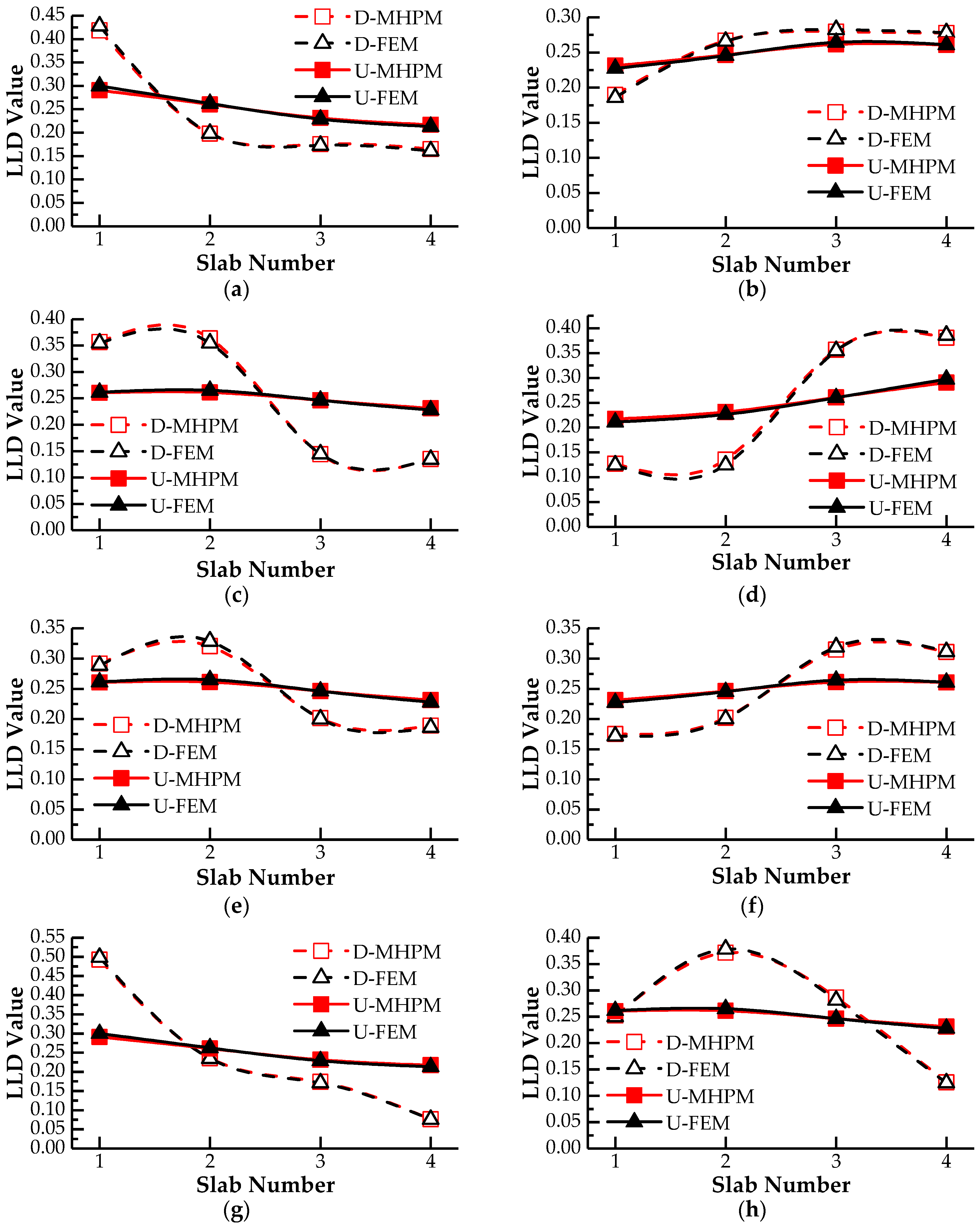
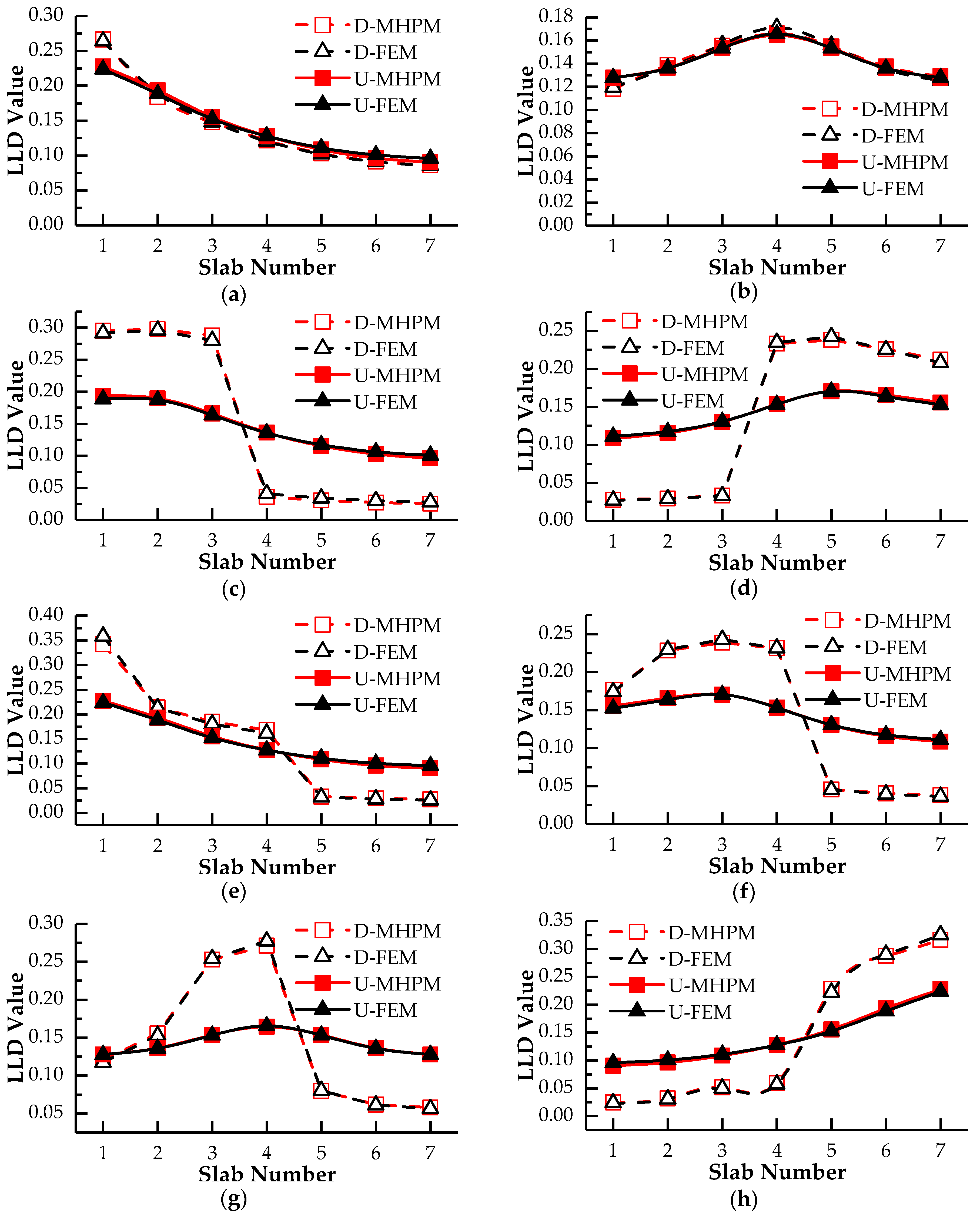
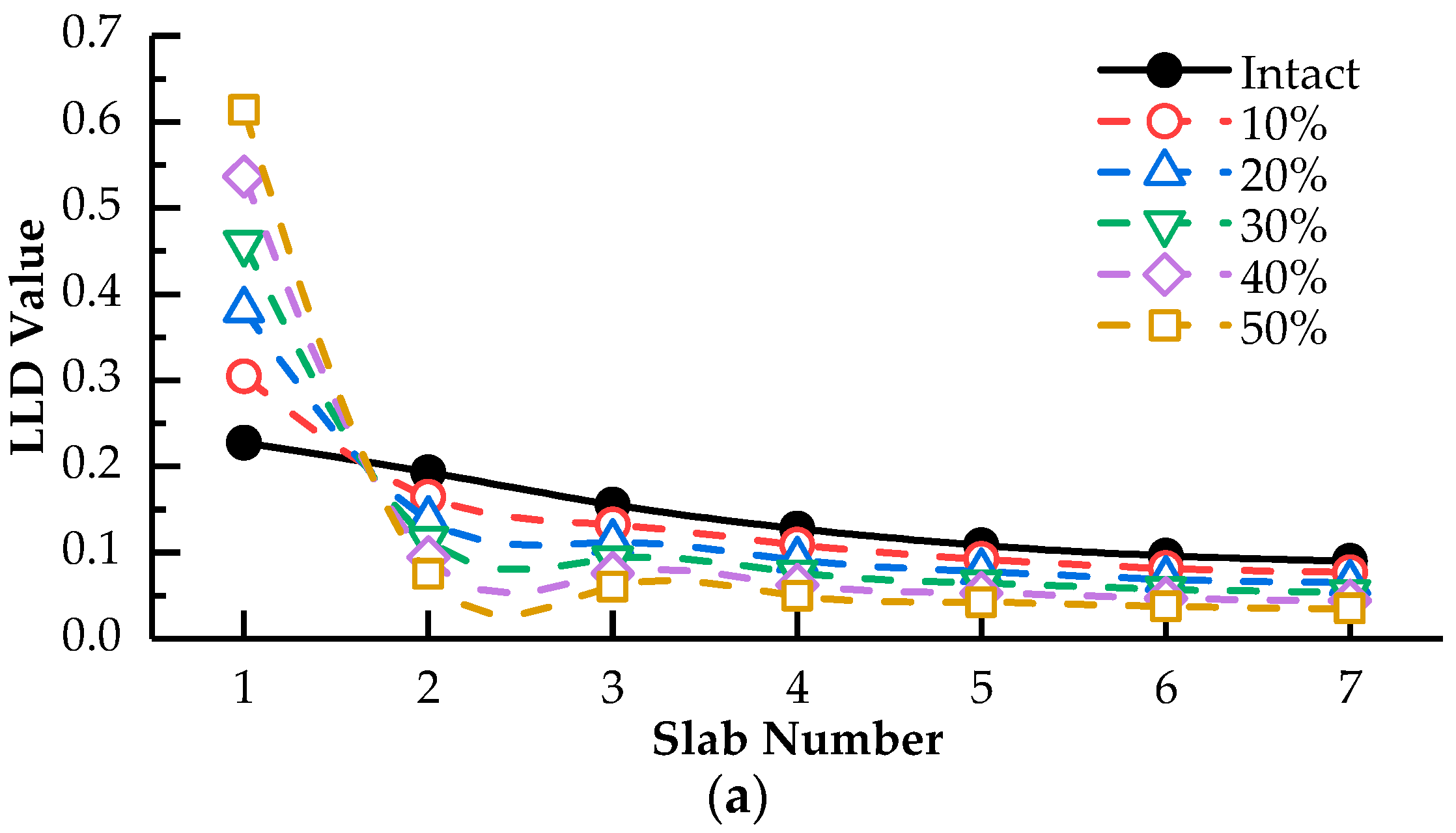
The damage factor through substitution of a relative displacement into the canonical equations can realize the simulation of hinge joint damage. The lateral load distribution influence line calculated by modified hinge plate method coincided with the result computed by the finite element method. The maximum error of damage cases in this study by modified hinge plate method was less than 1.9%.

(2)

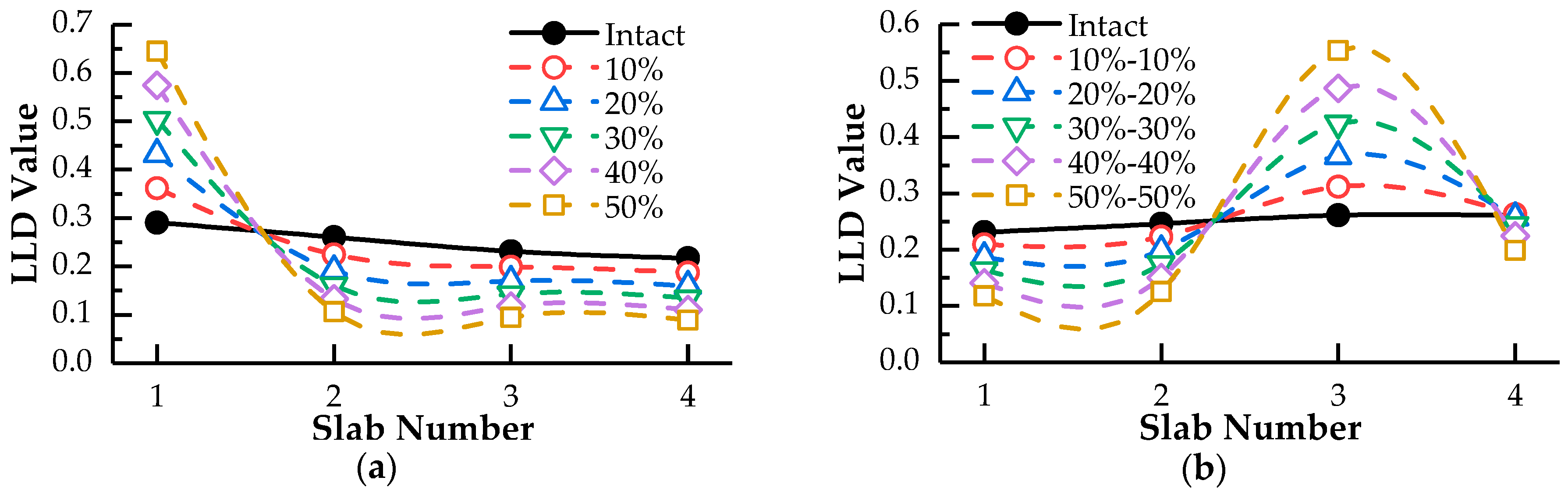
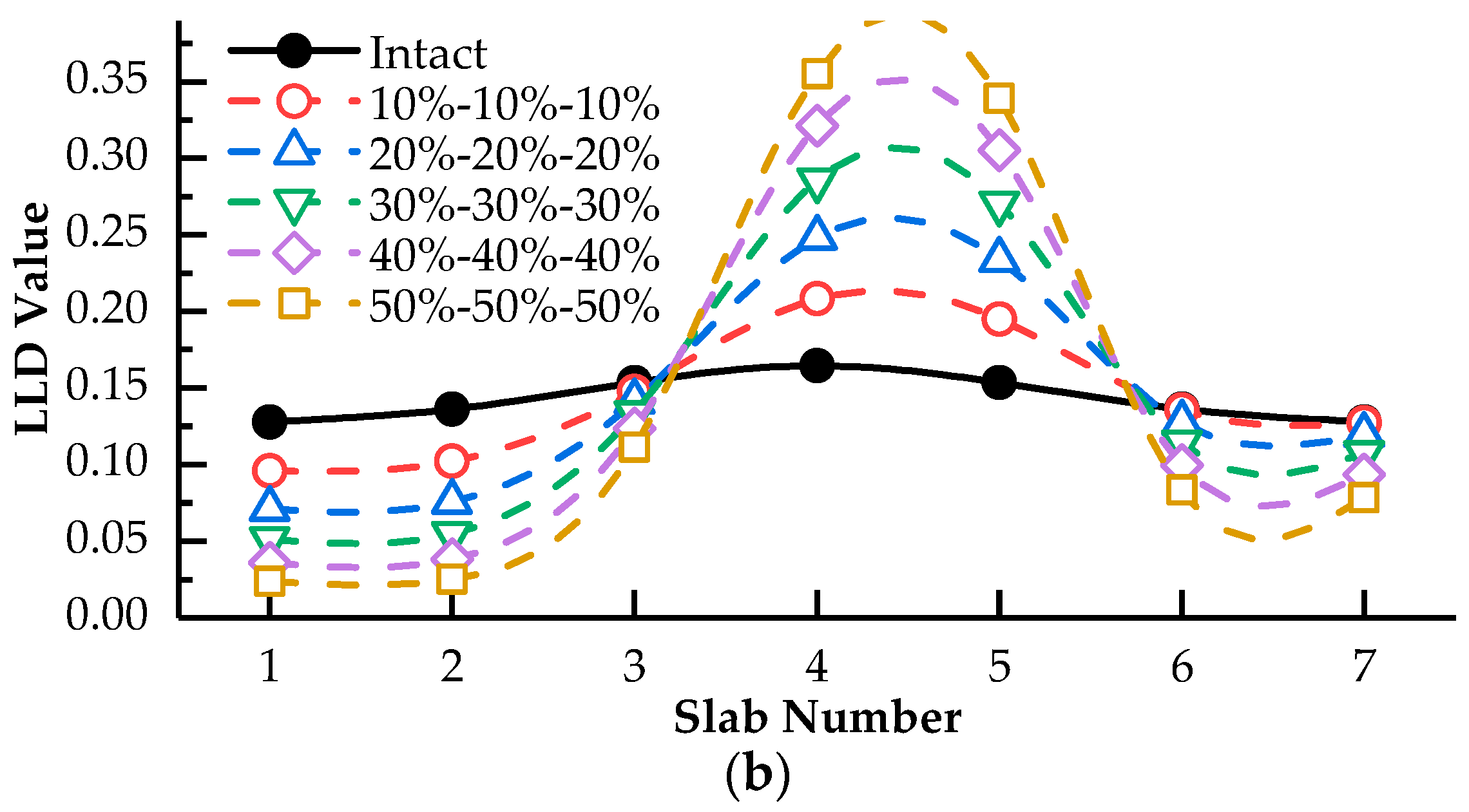
Hinge joint damage can lead to cross phenomenon of lateral load distribution influence lines, which is suitable for the damage localization of hinged-slab bridges with single hinge damage. Moreover, the offset degree of lateral load distribution influence line is proportional to damage degrees, which can realize the qualitative assessment of hinge damage. However, cross phenomenon is not effective to identify the damage location with multiple hinge damages.

(3)

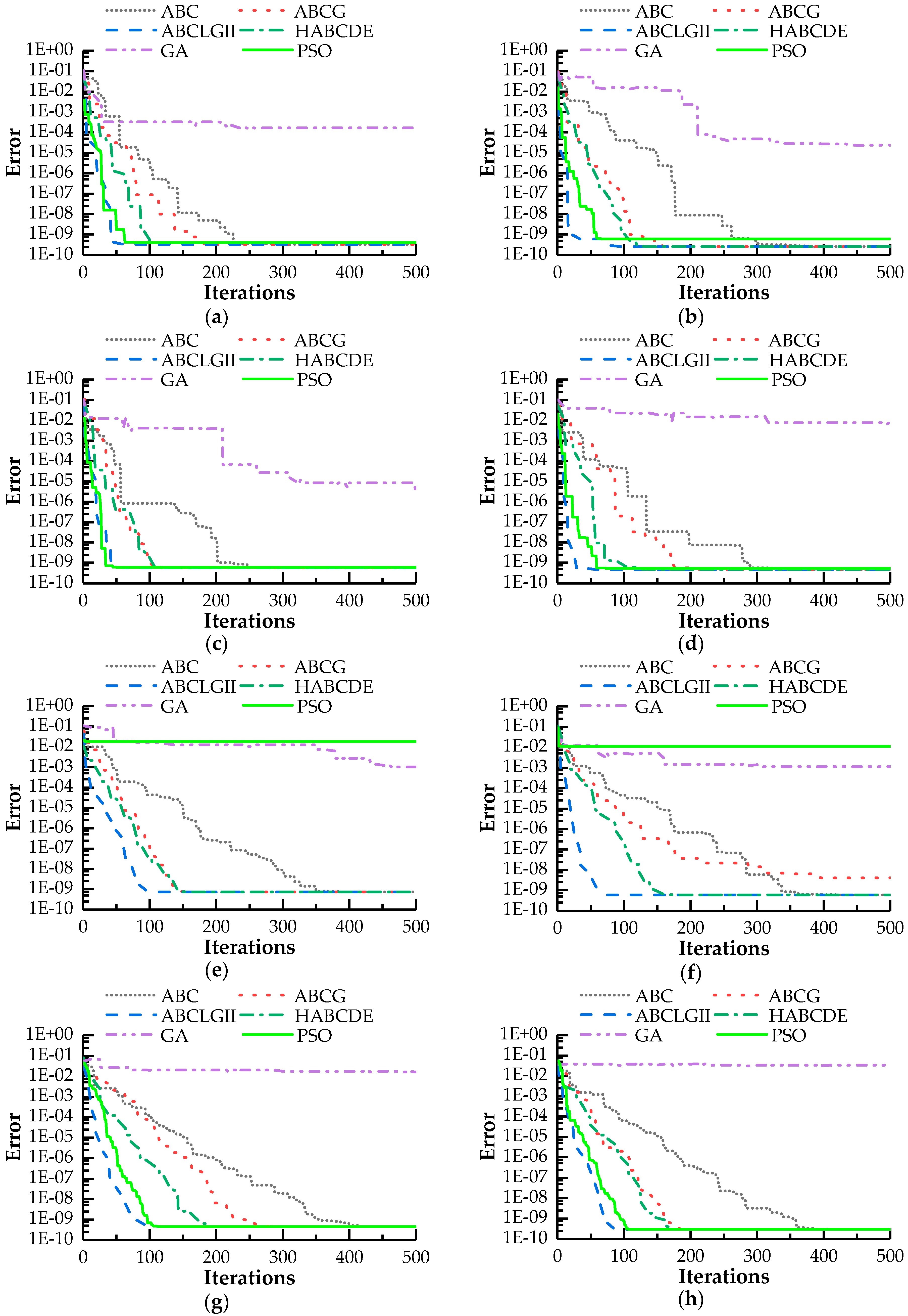
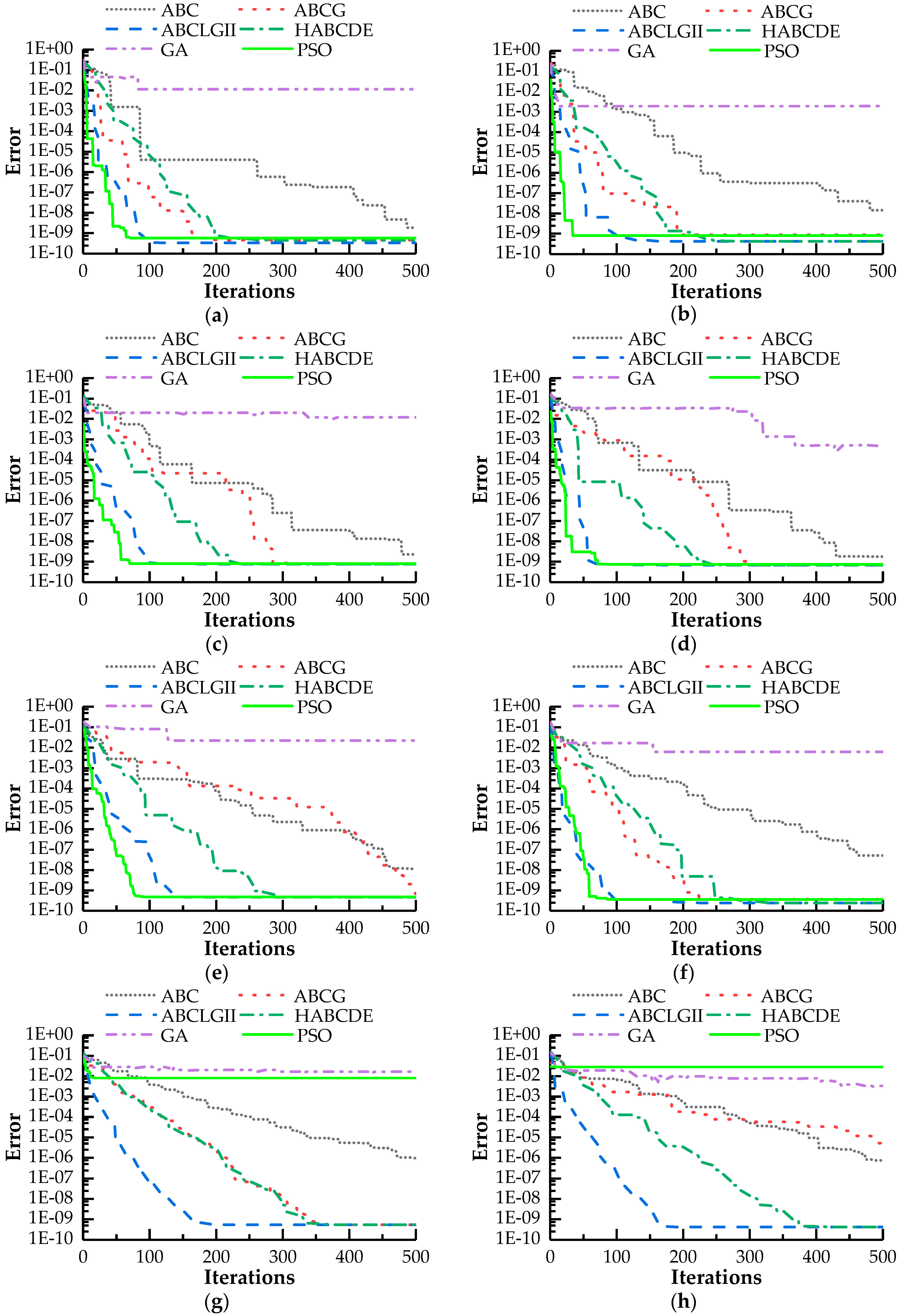
Original and improved artificial bee colony algorithms successfully identified the location and degree of hinge joint damages, of which the maximum error did not exceed 4.72 × 10⁻⁶. Based on ABCLGII and HABCDE, the algorithms had the lowest time cost (less than 70 s). Moreover, ABCLGII converged after 100 iterations approximately, while the others did not. So ABCLGII is the most suitable for the proposed damage identification algorithm among artificial bee colony algorithms in this work.

(4)

The results of comparison with particle swarm optimization and genetic algorithm revealed that both PSO and GA converged after 100 iterations at most and the time costs of them were no more than 30 s, which presented satisfactory convergence speed and time cost. However, the accuracy of damage identification algorithm based on PSO was not stable; namely, the minimum and maximum errors were 1 × 10⁻⁹ for single damage condition and 0.028 for multiple hinge damages, respectively. As for GA, its error fluctuated between 0.0005 and 0.022, which demonstrated it had the most unsatisfactory identification results among these methods.

(5)

It demonstrated again that the proposed algorithm was accurate through comparison with methods in the literature [19,20]. The former algorithm had zero error while the latter ones had larger errors ranging from 0.003 to 0.164. Even the latter algorithms identified the damage degree and location improperly.

The proposed algorithm presents good performances for hinge joint damage identification, but there are still some barriers for it, such as the computation time of the algorithm and the cost and efficiency of field experiment. In the future, the damage identification algorithm should be improved to reduce the high time cost. Furthermore, we will present a new field experiment method, which can measure the LLD influence line effectively and economically, as well as verify the performance of the proposed algorithm in actual engineering.

References

1. Heo, G.; Kim, C.; Jeon, S.; Jeon, J. An experimental study of a data compression technology-based intelligent data acquisition (IDAQ) system for structural health monitoring of a long-span bridge. Appl. Sci. 2018, 8, 361. [Google Scholar] [CrossRef]
2. Amezquita-Sanchez, J.P.; Adeli, H. Signal processing techniques for vibration-based health monitoring of smart structures. Arch. Comput. Method Eng. 2016, 23, 1–15. [Google Scholar] [CrossRef]
3. Satpal, S.B.; Guha, A.; Banerjee, S. Damage identification in aluminum beams using support vector machine: Numerical and experimental studies. Struct. Control Health 2016, 23, 446–457. [Google Scholar] [CrossRef]
4. Fan, W.; Qiao, P.Z. Vibration-based damage identification methods: A review and comparative study. Struct. Health Monit. 2011, 10, 83–111. [Google Scholar] [CrossRef]
5. Qin, S.Q.; Zhang, Y.Z.; Zhou, Y.L.; Kang, J.T. Dynamic model updating for bridge structures using the kriging model and PSO algorithm ensemble with higher vibration modes. Sensors 2018, 18, 1879. [Google Scholar] [CrossRef] [PubMed]
6. Blachowski, B.; An, Y.; Spencer, B.F., Jr.; Ou, J. Axial strain accelerations approach for damage localization in statically determinate truss structures. Comput.-Aided Civ. Inf. 2017, 32, 304–318. [Google Scholar] [CrossRef]
7. Kim, C.-W.; Chang, K.-C.; Kitauchi, S.; McGetrick, P.J. A field experiment on a steel gerber-truss bridge for damage detection utilizing vehicle-induced vibrations. Struct. Health Monit. 2016, 15, 174–192. [Google Scholar] [CrossRef]
8. Russo, F.M.; Wipf, T.J.; Klaiber, F.W.; Trb, T.R.B. Diagnostic load tests of a prestressed concrete bridge damaged by overheight vehicle impact. In Proceedings of the Fifth International Bridge Engineering Conference, TAMPA, FL, USA, 3–5 April 2000. [Google Scholar]
9. Chung, W.; Liu, J.; Sotelino, E.D. Influence of secondary elements and deck cracking on the lateral load distribution of steel girder bridges. J. Bridge Eng. 2006, 11, 178–187. [Google Scholar] [CrossRef]
10. Al-Saidy, A.H.; Klaiber, F.W.; Wipf, T.J.; Al-Jabri, K.S.; Al-Nuaimi, A.S. Parametric study on the behavior of short span composite bridge girders strengthened with carbon fiber reinforced polymer plates. Constr. Build. Mater. 2008, 22, 729–737. [Google Scholar] [CrossRef]
11. Kim, Y.J.; Green, M.F.; Fallis, G.J. Repair of bridge girder damaged by impact loads with prestressed CFRP sheets. J. Bridge Eng. 2008, 13, 15–23. [Google Scholar] [CrossRef]
12. Azimi, H.; Sennah, K. Parametric effects on evaluation of an impact-damaged prestressed concrete bridge girder repaired by externally bonded carbon-fiber-reinforced polymer sheets. J. Perform. Constr. Facil. 2015, 29, 1–12. [Google Scholar] [CrossRef]
13. Yao, L.S. Bridge Engineering, 2nd ed.; China Communicaitons Press: Beijing, China, 2010; pp. 128–142. ISBN 978-7-114-07042-6. (In Chinese) [Google Scholar]
14. American Association of State Highway and Transportation Officials (AASHTO). AASHTO Standard Specifications for Highway Bridges, 16th ed.; American Association of State Highway and Transportation Officials, Inc.: Washington, DC, USA, 1996; ISBN 1-56051-040-4. [Google Scholar]
15. American Association of State Highway and Transportation Officials (AASHTO). AASHTO LRFD Bridge Design Specifications, 6th ed.; American Association of State Highway and Transportation Officials, Inc.: Washington, DC, USA, 2012; ISBN 978-1-56051-523-4. [Google Scholar]
16. Huo, X.S.; Wasserman, E.P.; Iqbal, R.A. Simplified method for calculating lateral distribution factors for live load shear. J. Bridge Eng. 2005, 10, 544–554. [Google Scholar] [CrossRef]
17. Wang, W.Y.; Zhang, C.; Wan, S. Study on transverse load distribution of hinged hollow beam. In Proceedings of the 2017 4th International Conference on Advanced Materials, Mechanics and Structural Engineering, Tianjin, China, 22–24 September 2017. [Google Scholar]
18. Jiao, Y.B.; Liu, H.B.; Wang, X.Q.; Luo, G.B. Modal property-based approach for lateral distribution evaluation of intact and damaged reinforced concrete bridge. In Proceedings of the 10th International Workshop on Structural Health Monitoring, Stanford, CA, USA, 1–3 September 2015; pp. 2911–2918. [Google Scholar]
19. Wei, B.L.; Deng, M.Y. Computional method analysis for transverse load distribution of damage bridge. J. Henan Polytech. Univ. 2015, 34, 102–108. [Google Scholar] [CrossRef]
20. Cheng, C.; Shen, C.W.; Xu, L. The hinged-jointed plate method for calculating transverse load distribution on a damaged bridge. J. Wuhan Univ. Technol. 2004, 28, 229–231. (In Chinese) [Google Scholar]
21. Conde, B.; Drosopoulos, G.A.; Stavroulakis, G.E.; Riveiro, B.; Stavroulaki, M.E. Inverse analysis of masonry arch bridges for damaged condition investigation: Application on kakodiki bridge. Eng. Struct. 2016, 127, 388–401. [Google Scholar] [CrossRef]
22. Santos, A.; Silva, M.; Santos, R.; Figueiredo, E.; Sales, C.; Costa, J.C.W.A. A global expectation-maximization based on memetic swarm optimization for structural damage detection. Struct. Health Monit. 2016, 15, 610–625. [Google Scholar] [CrossRef]
23. Wei, Z.T.; Liu, J.K.; Lu, Z.R. Structural damage detection using improved particle swarm optimization. Inverse Probl. Sci. Eng. 2018, 26, 792–810. [Google Scholar] [CrossRef]
24. Yang, Z.B.; Chen, X.F.; Xie, Y.; Miao, H.H.; Gao, J.J.; Qi, K.Z. Hybrid two-step method of damage detection for plate-like structures. Struct. Control Health 2016, 23, 267–285. [Google Scholar] [CrossRef]
25. Casciati, S.; Elia, L. Damage localization in a cable-stayed bridge via bio-inspired metaheuristic tools. Struct. Control Health 2017, 24. [Google Scholar] [CrossRef]
26. Antonelli, A.; Giarnetti, S.; Leccese, F. Enhanced PLL system for harmonic analysis through genetic algorithm application. In Proceedings of the International Conference on Environment and Electrical Engineering, Venice, Italy, 18–25 May 2012; pp. 328–333. [Google Scholar] [CrossRef]
27. Hou, W.; Jin, Y.; Zhu, C.; Li, G. A novel maximum power point tracking algorithm based on glowworm swarm optimization for photovoltaic systems. Int. J. Photoenergy 2016. [Google Scholar] [CrossRef]
28. Karaboga, D.; Basturk, B. On the performance of artificial bee colony (ABC) algorithm. Appl. Soft Comput. 2008, 8, 687–697. [Google Scholar] [CrossRef]
29. Karaboga, D.; Akay, B. A comparative study of artificial bee colony algorithm. Appl. Math. Comput. 2009, 214, 108–132. [Google Scholar] [CrossRef]
30. Pham, D.T.; Castellani, M. Benchmarking and comparison of nature-inspired population-based continuous optimisation algorithms. Soft Comput. 2014, 18, 871–903. [Google Scholar] [CrossRef]
31. Sun, H.; Lus, H.; Betti, R. Identification of structural models using a modified artificial bee colony algorithm. Comput. Struct. 2013, 116, 59–74. [Google Scholar] [CrossRef]
32. Xu, H.J.; Ding, Z.H.; Lu, Z.R.; Liu, J.K. Structural damage detection based on chaotic artificial bee colony algorithm. Struct. Eng. Mech. 2015, 55, 1223–1239. [Google Scholar] [CrossRef]
33. Karaboga, D. An Idea Based on Honey Bee Swarm for Numerical Optimization. Ph.D. Thesis, Erciyes University, Kayseri, Turkey, 2005. [Google Scholar]
34. Gao, W.F.; Liu, S.Y.; Huang, L.L. Enhancing artificial bee colony algorithm using more information-based search equations. Inf. Sci. 2014, 270, 112–133. [Google Scholar] [CrossRef]
35. Akay, B.; Karaboga, D. A modified artificial bee colony algorithm for real-parameter optimization. Inf. Sci. 2012, 192, 120–142. [Google Scholar] [CrossRef]
36. Pang, B.; Song, Y.; Zhang, C.; Wang, H.; Yang, R. A modified artificial bee colony algorithm based on the self-learning mechanism. Algorithms 2018, 11, 78. [Google Scholar] [CrossRef]
37. Karaboga, D.; Gorkemli, B. A quick artificial bee colony (QABC) algorithm and its performance on optimization problems. Appl. Soft Comput. 2014, 23, 227–238. [Google Scholar] [CrossRef]
38. Jadon, S.S.; Tiwari, R.; Sharma, H.; Bansal, J.C. Hybrid artificial bee colony algorithm with differential evolution. Appl. Soft Comput. 2017, 58, 11–24. [Google Scholar] [CrossRef]
39. Xiang, W.L.; Meng, X.L.; Li, Y.Z.; He, R.C.; An, M.Q. An improved artificial bee colony algorithm based on the gravity model. Inf. Sci. 2018, 429, 49–71. [Google Scholar] [CrossRef]
40. Liu, Q.Z.; Zhu, M.M.; Li, G.H.; Wang, W.J.; Cui, L.Z.; Chen, J.Y.; Lu, J. A novel artificial bee colony algorithm with local and global information interaction. Appl. Soft Comput. 2018, 62, 702–735. [Google Scholar] [CrossRef]
41. Yildiz, A.R. A new hybrid artificial bee colony algorithm for robust optimal design and manufacturing. Appl. Soft Comput. 2013, 13, 2906–2912. [Google Scholar] [CrossRef]
42. Li, G.H.; Shi, D. Calculation of Lateral Load Distribution of Highway Bridges, 2nd ed.; China Communicaitons Press: Beijing, China, 1990; pp. 87–116. (In Chinese) [Google Scholar]
43. Ravanfar, S.A.; Razak, H.A.; Ismail, Z.; Hakim, S.J.S. A two-step damage identification approach for beam structures based on wavelet transform and genetic algorithm. Meccanica 2016, 51, 635–653. [Google Scholar] [CrossRef]
44. Liu, H.B.; Wang, X.Q.; Jiao, Y.B. Damage identification for irregular-shaped bridge based on fuzzy c-means clustering improved by particle swarm optimization algorithm. J. Vibroeng. 2016, 18, 2149–2166. [Google Scholar] [CrossRef]
Figure 1. Hinge joint damage on a simply supported slab bridge.
Algorithms 11 00198 g001
Figure 2. The force diagram of simply supported hinged-slab bridge.
Algorithms 11 00198 g002
Figure 3. The basic system for shear analysis: (a) unit external force loaded on side slab; (b) unit external force loaded on internal slab.
Algorithms 11 00198 g003
Figure 4. Illustration of the damage factor for ith hinge.
Algorithms 11 00198 g004
Figure 5. Illustration of hinge joint forms: (a) general cross-sections of the hinge joint; (b) simplified hinge joint; (c) hinge joint simulation in finite element method (FEM).
Algorithms 11 00198 g005aAlgorithms 11 00198 g005b
Figure 6. FEM of simply supported slab bridge: (a) composed of four slabs; (b) composed of seven slabs.
Algorithms 11 00198 g006
Figure 7. LLD influence lines under damage and intact cases of 4-slab bridge: (a) case 1: slab 1; (b) case 1: slab 3; (c) case 2: slab 2; (d) case 2: slab 4; (e) case 3: slab 2; (f) case 3: slab 3; (g) case 4: slab 1; (h) case 4: slab 2.
Algorithms 11 00198 g007
Figure 8. LLD influence lines under damage and intact cases of 7-slab bridge: (a) case 5: slab 1; (b) case 5: slab 4; (c) case 6: slab 2; (d) case 6: slab 5; (e) case 7: slab 1; (f) case 7: slab 3; (g) case 8: slab 4; (h) case 8: slab 7.
Algorithms 11 00198 g008
Figure 9. LLDs for a simply supported bridge with 4 slabs under different damage conditions: (a) LLD of slab 1 with hinge joint 1 damage; (b) LLD of slab 3 with hinge joints 2 and 3 damages.
Algorithms 11 00198 g009
Figure 10. LLDs for a simply supported bridge with 7 slabs under different damage conditions: (a) LLD of slab 1 with hinge joint 1 damage; (b) LLD of slab 4 with hinge joints 2, 3, and 5 damages.
Algorithms 11 00198 g010aAlgorithms 11 00198 g010b
Figure 11. The flowchart of damage identification of hinge joint damage based on the artificial bee colony (ABC) algorithm.
Algorithms 11 00198 g011
Figure 12. Iteration process of damage identification for cases 1 to 4: (a) case 1: slab 1; (b) case 1: slab 3; (c) case 2: slab 2; (d) case 2: slab 4; (e) case 3: slab 2; (f) case 3: slab 3; (g) case 4: slab 1; (h) case 4: slab 2.
Algorithms 11 00198 g012
Figure 13. Iteration process of damage identification for Case 5 to Case 8: (a) case 5: slab 1; (b) case 5: slab 4; (c) case 6: slab 2; (d) case 6: slab 5; (e) case 7: slab 1; (f) case 7: slab 3; (g) case 4: slab 4; (h) case 4: slab 7.
Algorithms 11 00198 g013