Article

Differential-Evolution-Based Coevolution Ant Colony Optimization Algorithm for Bayesian Network Structure Learning

1
Faculty of Information Technology, Beijing University of Technology, Beijing 100124, China
2
Engineering Research Center of Digital Community, Ministry of Education, Beijing 100124, China
3
Beijing Laboratory for Urban Mass Transit, Beijing 100124, China
*
Author to whom correspondence should be addressed.
Algorithms 2018, 11(11), 188; https://doi.org/10.3390/a11110188
Submission received: 17 October 2018 / Revised: 8 November 2018 / Accepted: 16 November 2018 / Published: 19 November 2018

Abstract

:
Learning the Bayesian networks (BNs) structure from data has received increasing attention. Many heuristic algorithms have been introduced to search for the optimal network that best matches the given training data set. To further improve the performance of ant colony optimization (ACO) in learning the BNs structure, this paper proposes a new improved coevolution ACO (coACO) algorithm, which uses the pheromone information as the cooperative factor and the differential evolution (DE) as the cooperative strategy. Different from the basic ACO, the coACO divides the entire ant colony into various sub-colonies (groups), among which DE operators are adopted to implement the cooperative evolutionary process. Experimental results demonstrate that the proposed coACO outperforms the basic ACO in learning the BN structure in terms of convergence and accuracy.

1. Introduction

The Bayesian network (BN) [1], which is also called the probabilistic belief network or the causal network [2], is a kind of graphical model and knowledge representation tool. BNs can efficiently give the probabilistic description of the dependence or independence relationships between a set of random variables. A BN is composed of a directed acyclic graphical structure and a set of probability parameters. The directed acyclic graphical structure represents the dependence relationships between various variables, and the corresponding probability parameters specify their degree of dependence. Recently, learning the BN structure from a dataset has received increasing attention [3], and researchers have introduced various learning algorithms to obtain the structure for BNs. According to the modeling type [3,4,5], these structure learning algorithms can be classified into methods based on detecting conditional independencies [6,7], also known as constraint-based methods, the “score+search” method [1,2,8,9,10,11,12,13], and the algorithms that combine the above two methods [14,15,16,17]. As to the score+search method, the BN structure learning is modelled as an optimization problem. A scoring metric is employed to evaluate how well the candidate network structure [3] matches the dataset. The better the candidate network structure matches the dataset, the higher the score. Thus, it can use the optimization technique to search for the network structure with the best score. However, searching for the optimum network for BNs is an NP-hard problem [5,18], which means those exact methods become unfeasible. Therefore, the approximate algorithms are very useful for quickly obtaining a sufficiently highly qualified network structure. The greedy search methods, including the K2 algorithm and many meta-heuristic methods, such as genetic algorithm (GA) [12], evolutionary programming (EP) [12] and particle swarm optimization (PSO) [14], are frequently used in solving the BN learning problem.
As a population-based meta-heuristic technique, ant colony optimization (ACO) also has been introduced successfully into the problem of BN structure learning from a dataset [1,2,8,14,15]. ACO, which was originally presented under the inspiration from the collective behavior of a real ant system [19,20], has already been applied to a wide range of optimization problems. Campos et al. [2] first introduced ACO to the problem of BN structure learning. They described all of the elements necessary to tackle the BN learning problem using ACO, and contrast experiments indicated that ACO shows better performance than the estimation of distribution algorithms (EDAs) as well as the greedy hill climbing (HC) algorithm. Based on the constraint-based local discovery algorithm, Pinto et al. [1] proposed a local discovery ACO by using the conditional dependence test max-min parents and children method. Ji et al. [15] proposed a hybrid method that combines ACO, the conditional independence test, and the simulated annealing (SA) strategy, and their hybrid ACO method outperforms the basic ACO in terms of computational time and searching capability. However, there are two drawbacks in the above ACO-based hybrid algorithms. Firstly, the conditional independence test can make the computation more complex and unreliable [3]. Secondly, when the number of variables is very large, the ACO-based algorithm will easily fall into the local optimal solution and result in a premature stagnation. To avoid the drawback caused by the conditional independence test, it is necessary to improve the inherent searching mechanism of the ACO algorithm.
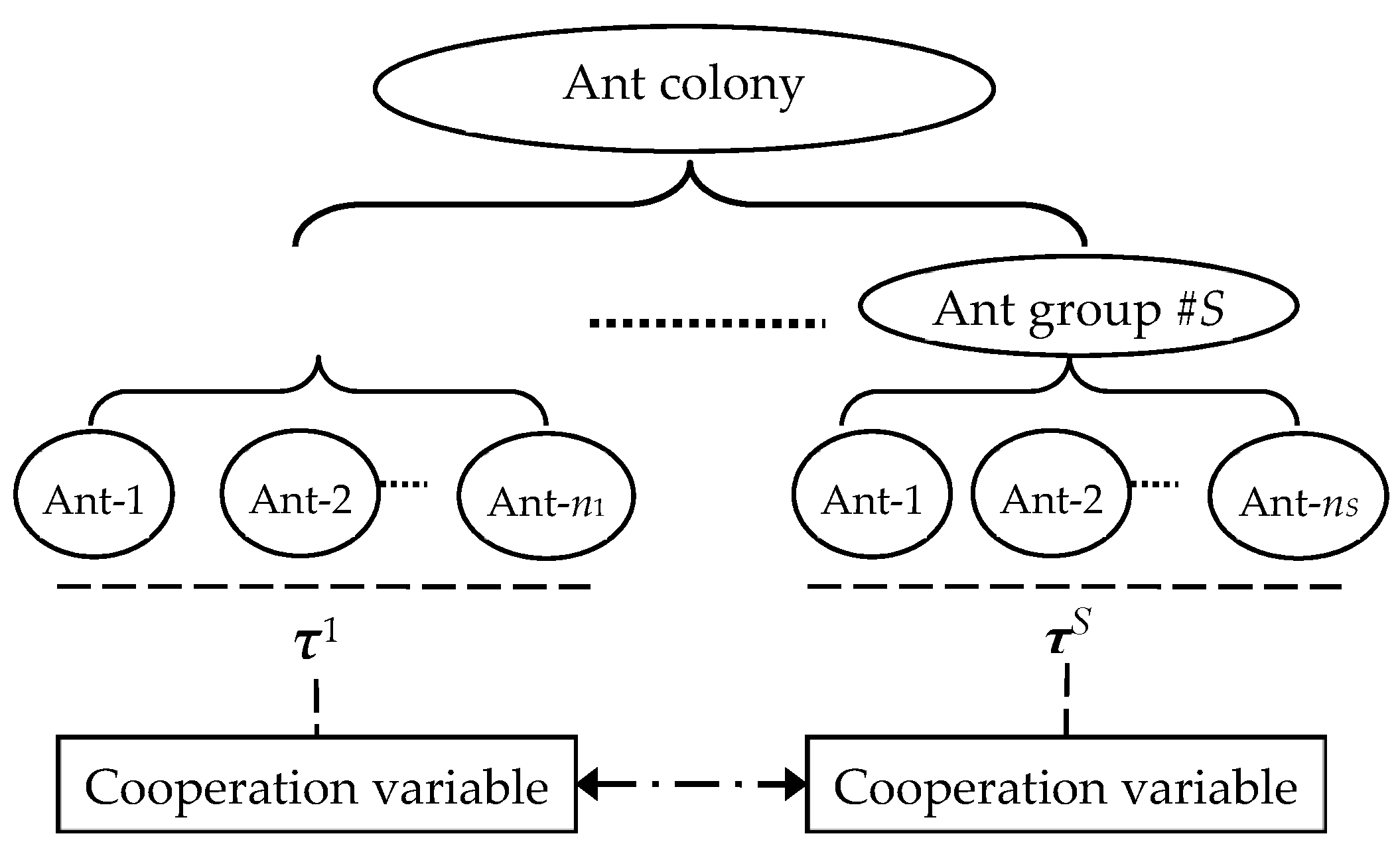
In this paper, we propose a kind of improved ACO to enhance the convergence and accuracy of the basic ACO in solving the problem of BN structure learning. The improved ACO divides the entire ant colony into several small sub-colonies, denoted as groups. In each ant group, ants perform respective actions, which leads to the entire ant group evolving forward according to the information within the group itself. Moreover, at the same time, among different groups, the information is also shared in the form of a cooperation variable, and all of the ant groups will evolve forward together using cooperative operations. The cooperative operations in the cooperative evolution process are based on the differential evolution (DE) algorithm [21,22], which leads the cooperative evolution process for all ant groups. The proposed improved ACO is denoted as coevolution ACO (coACO). Two features make the coACO algorithm interesting: (1) the grouping operator divides the entire ant colony into different ant groups, and, thus, the algorithm can carry out not only the social cooperation between ant individuals but also the cooperative interaction and information shared between ant groups; (2) the DE algorithm is employed to adjust the cooperation information and lead all ant groups to evolve toward the optimum in a cooperative manner.
In the rest of this paper, a problem description of the BN structure learning as well as the introduction of the ACO algorithm are given in Section 2. The proposed coACO algorithm and the detailed BN structure learning method are described in Section 3. Section 4 presents the test results. Section 5 concludes this paper.

2. Preliminaries

2.1. Problem of BN Structure Learning

A BN is a graphical tool to represent the n-dimensional probability distribution. It can be described by a directed acyclic graph (DAG) GX, A, Θ>. In G, each node Xi X represents a random variable of interest, while each arc aij A represents a direct dependence relationship between the variables Xi and Xj. In addition, the parameter θi = P(Xi|πi), where Θ = {θi}, denotes the conditional probability distribution of Xi given its parent set πi. From the conditional distributions, the joint probability can be uniquely determined by
P ( X 1 , X 2 , , X n ) = i = 1 n P ( X i | π i ) .  
Given a training database D = {x1, x2, , xm} composed of m cases and each case contains n variables, where xi is an instance of domain variable X, the problem of the BN structure learning is to find the BN topology structure that best matches the dataset D.
As noted previously, algorithms for learning the BN structure from data mainly include the constraint-based methods and the score+search methods. Based on a dependency analysis, the existing approaches are close to the semantics of BNs and relatively simpler to implement [8]. However, it is hard to ensure the precision of the obtained structure. Furthermore, the computation for high-order tests is complex and unreliable. For this reason, most of the developed structure learning algorithms fall into the latter, namely the score+search methods [3,5], which treat the problem of BN structure learning as a combinatorial optimization problem.
The BN structure learning based on score+search methods firstly uses a scoring metric to evaluate how well the candidate BN structure matches the given dataset, and then finds the network structure with the maximum score. Popular scoring metrics include Akaike’s information criterion (AIC), the Bayesian information criterion (BIC), the minimum description length (MDL) score, and the Bayesian Dirichlet equivalence (BDe) metric (usually called the K2 metric) [3]. Here, the BIC scoring metric, which comes from the penalized maximum likelihood, is used as the structure to identify the dataset matching degree as follows:
P ( B S | D ) = i = 1 n j = 1 q i k = 1 r i ( N i j k N i j ) N i j k f ( m ) dim ( B S )  
where, BS is the candidate BN structure;
ri is the number of possible values for the variable Xi;
qi is the number of possible configurations instantiations for its parents πi;
Nijk is the number of cases in D in which variable Xi has its k-th value, πi is instantiated to its j-th value, and N i j = k = 1 r i N i j k ;
dim ( B S ) = i = 1 m q i ( r i 1 ) is the dimension (the number of parameters needed to specify the model) of the BN; and f(m) is the non-negative penalization function that depends on the size of the dataset and can be computed as f(m) = 0.5·log m.
Using f(BS, D) instead of P(BS|D), the BIC scoring metric [3] is defined as:
f B I C ( B S , D ) = log ( i = 1 n j = 1 q i k = 1 r i ( N i j k N i j ) N i j k ) f ( m ) dim ( B S ) = i = 1 n f B I C ( x i , π i )  
where
f B I C ( x i , π i ) = j = 1 q i k = 1 r i ( N i j k log N i j k N i j ) 1 2 log m q i ( r i 1 ) .  
One desirable and important feature of scoring metrics is their decomposability in the presence of full data, and (3) shows that the BIC metric used here is decomposable. With the decomposable metric, a local search procedure that changes one arc at each move can efficiently evaluate the improvement obtained by this change [2,3], because it can reuse most of the computations made in previous stages. Moreover, the score of a BN can be computed as the combination of scores obtained for smaller factors.

2.2. ACO

As a representative bio-inspired meta-heuristic algorithm, ACO was firstly put forward by Dorigo in the 1990s [19] to solve the travel salesman problem (TSP). Till now, ACO has been proven to be a more common framework for various optimization problems in a wide range of fields [23,24,25], such as job-shop scheduling, data mining, routing problems, and other complex optimization problems. When observing the foraging behavior of real ant colonies, researchers discovered that real ants can deposit a chemical substance, called a pheromone, while walking. The pheromone can be accumulative and evaporative, through which the ant colony can carry on indirect communication and finally achieve the cooperative goal. Ants can smell the pheromone and choose their way, in a probabilistic way, based on the amount of pheromone. The larger the amount of pheromone deposited on a route, the greater the probability that ants select the route. Meanwhile, on the shorter route that ants travel, the pheromone accumulates faster than on the longer routes. Thus, the faster the amount of pheromone increases on the shorter route, then the greater the probability that the ants travel this route. In the initial stage when the pheromone is absent, ants choose their routes fully randomly, but after a transitory period the shortest routes will be more and more frequently visited and pheromone will accumulate faster and faster on them, which in turn will attract more and more ants to choose these routes.
The mathematical model of ACO is described as follows. Let Mant be the number of ants, and the matrix τ(t) = {τij(t)} be the pheromone, of which the element τij(t) is the level of pheromone deposited on the arc from node i to node j, at time t. The initial level of pheromone on each directed arc is a constant value, i.e., τij(0) = τ0. Each ant builds a possible solution to the problem by moving through a finite sequence of neighbor nodes, and these moves are directed by the ant’s internal state, problem-specific local information, and the shared information about the pheromone [19]. For the k-th ant located at the i-th node, it will move to the next j-th node with the transition probability:
p i j k ( t ) = { [ τ i j ( t ) ] α [ η i j ] β u a l l o w e d k [ τ i u ( t ) ] α [ η i u ] β if   j a l l o w e d k 0 otherwise  
where ηij represents the heuristic information about the problem, allowedk denotes the feasible domain of the k-th ant at the i-th node, and α and β are parameters that determine the relative importance of the pheromone with respect to the heuristic information.
In addition, in order to achieve a trade-off between exploitation and exploration [2], a different transition rule is introduced and the next node j is selected as:
j = { arg max u a l l o w e d k {   [ τ i u ( t ) ] [ η i u ] β } if   q q 0 J otherwise  
where q is a random number uniformly distributed in [ 0 , 1 ] ; q0 [0,1] is the parameter that determines the relative importance of exploitation versus exploration; and J is a node randomly selected according to the transition probability in (1) with α = 1.
As the ants move and build the possible solutions, the pheromone matrix is updated according to both the global updating and local updating processes [20]. As to the local updating process when building the solution, if an ant moves from node i to node j, then the pheromone level on the corresponding arc ij is updated as follows:
τ i j ( 1 ψ ) τ i j + ψ τ 0  
where τ0 is the initial pheromone level on all arcs, and ψ (0,1] denotes the parameter that can control the pheromone evaporation. After all ants have constructed a solution, only the ant that obtains the best solution can reinforce the pheromone level on the arcs, which constitute the best solution, S+, obtained by the ant colony so far. The global updating rule can be expressed by
τ i j ( t + 1 ) = ( 1 ρ ) τ i j ( t ) + ρ Δ τ i j  
Δ τ i j = { 1 f ( S + ) if   { i , j } S + τ i j otherwise  
where ρ (0,1] is the parameter that can control the pheromone evaporation, and f(S+) is the cost associated with the best solution S+. The following Algorithm 1 shows the complete algorithm of ACO applied to optimization problems [19].
Algorithm 1: ACO algorithm.
/*Initialization */
1Set the iteration counter g = 0;
2Generate Mant ants, and initialize the pheromone matrix;
/* Iterative search */
3while termination criteria are not satisfied do
4 iteration counter g = g + 1
5for i = 1: Mant do
  /* Build a possible solution */
6  while the solution is not completed do
7   Randomly select a state/node according to the probabilistic transition rule;
8   Update the pheromone according to the local updating rule;
9  end while
10end for
 /* Pheromone updating */
11 Select the best solution and perform the global updating process;
12end while
13Return the best solution S+.

2.3. ACO Applied to BNs

Using the basic ACO algorithm, the best network can be found in the space of possible networks based on the score+search framework, [1,2]. Beginning with a blank network, the ant colony progressively searches for good single-step changes to build a complete BN. Each ant connects randomly two variables and determines whether the arc should be included in the BN structure. As the construction process that is illustrated in Figure 1 [2,14,15], the ant uses the incremental construction of the solution starting from a blank network G0 through connecting an arc aij = {Xi→Xj} and then adding it to the current network, i.e., Gh+1 = Ghaij. When no arc can be added to achieve a higher score of the BN structure, the construction process of the ant will be stopped with obtaining the final solution Gg. The pheromone placed on all candidate arcs together with the heuristic information are used to guide the network construction process. The random rule that the ant k selects the arc aij from the current optional arcs is
a i j = { arg max e a l l o w e d k {   [ τ e ( t ) ] [ η e ( t ) ] β } if   q q 0 A i j otherwise  
where Aij are the arcs randomly selected according to the following probabilities:
p i j k ( t ) = { [ τ i j ( t ) ] [ η i j ( t ) ] β E u v a l l o w e d k [ τ u v ( t ) ] [ η u v ( t ) ] β if   a i j a l l o w e d k 0 otherwise  
where allowedk is the set composed of all candidate arcs that do not create a directed cycle and have the positive heuristic information. q0 is the threshold value that is set by the user.
The maximum objective function of ACO is the BIC scoring metric in (3). Thus, the heuristic information ηij of the arc aij at time t is defined as
η i j = f B I C ( X i , π i X j ) f B I C ( X i , π i )  
The pheromone level τij on the arc aij changes according to the local and global updating rules as described in (7) and (8), while the increment is competed by
Δ τ i j = { 1 | f B I C ( G + , D ) | if   a i j G + τ i j otherwise  
where G+ is the best BN structure found by all ants so far. The basic ACO algorithm applied to learning the BN structure is presented in Algorithm 2 [2].
Algorithm 2: Basic ACO based BN learning.
/* Initialization */
1Set the iteration counter t = 0;
2Generate Mant ants;
3Initialize the pheromone matrix τ(0): for all arcs aij, set τij(0) = τ0;
4Set G+ be an empty graph;
/* Iterative search */
5while termination criteria are not satisfied do
6 iteration counter t = t + 1
7for k = 1:Mant do
8  Generate an empty network Gk: for i = 1 to n, do πi = ϕ;
9  Calculate the heuristic information: for i, j = 1 to n (Ij) do ηij = fBIC(Xi, Xj) − fBIC(Xi, ϕ);
10  while ηij > 0 do
   /* Add an arc */
11   Select an arc aij from the feasible domain allowed according to (9) and (10);
12   if ηij > 0 then πi = πi∪{Xj} and construct the network Gk = Gkaji;
13   Set ηij = −∞;
   /* Avoiding directed cycles */
14   for u, v = 1 to n do
15    if Gkauv includes a directed cycle, then ηuv = −∞;
16   end for
   /* Calculation the heuristic information */
17   for u = 1 to n do
18    if ηiu > −∞ then ηiu = fBIC(Xi, πi∪{Xu}) − fBIC(Xi, πi);
19   end for
   /* Local updating */
20   Update the pheromone: τij = (1 − ψ)·τij + ψ·τ0;
   /* Local updating */
21   Update the pheromone: τij = (1 − ψ)·τij + ψ·τ0;
22  end while
23end for
24 /* Pheromone update */
26 Select Gt = arg max fBIC(Gk, D)
27if fBIC(Gt, D) ≥ fBIC(G+, D), then G+ = Gt
28 Update the pheromone matrix according to (8) and (12) using fBIC(G+, D)
29end while
30Return the best BN structure G+.

3. Method

This paper introduces a new improved algorithm, coACO, to solve the BN structure-learning problem. The coACO incorporates several coevolution operators to improve the performance of the basic ACO. Firstly, the entire ant colony is divided into S independent ant groups, and the number of groups is set as ns, s = 1, …, S, as shown in Figure 2. DE is one of the best evolutionary algorithms for solving the real-valued test function suite of the First International Contest on Evolutionary Optimization (1st ICEO) [22]. Therefore, the DE strategies [26,27] are used to guide the coevolution process for all ant groups. As is mentioned in the above section, the pheromone plays an important role in the exploration and exploitation of the ant colony for constructing the solution. A reasonable distribution of the pheromone can directly affect ants to explore their solutions. Thereby, the pheromone level is chosen as the cooperative object shared by all ant groups in the coACO.
For each ant group, the pheromone level is denoted as the matrix τs(t) = {τijs(t)}, s = 1, …, S. Each ant group communicates with other groups and coordinates its evolution process using the pheromone as the cooperative variable. The coACO introduces coordination operations, which are based on DE, to affect the pheromone, which leads to the achievement of a more reasonable distribution of the pheromone for each ant group.
The DE-based coordination operations contain mutation, crossover, and selection operators [21]. The first one is the mutation operator, which is implemented as follows:
u s = τ r 1 + F × ( τ r 2 τ r 3 )  
where us(t) = {uijs(t)}, s = 1, …, S, is the donor pheromone matrix. τ r 1 , τ r 2 , and τ r 3 are three different pheromone matrixes that are randomly selected from the ant groups, namely r1r2r3s. The real number F is a positive parameter between [0,2], called the mutation factor, which controls the amplification of the differential variation ( τ r 2 τ r 3 ) .
The second one is the crossover operator, which is performed as follows:
v i j s = { u i j s if   r i j c r τ i j s otherwise  
where rij is a random value generated for each arc aij in accordance with a uniform distribution over [0,1], cr is the given crossover rate within (0,1), and the obtained vs(t) = {vijs(t)} is the trial pheromone matrix. Figure 3 describes the crossover process of the pheromone matrixes.
The third operator is the greedy selection, which is performed as follows:
τ s ( t + 1 ) = { v s ( t ) if   f ( v s ( t ) ) f ( τ s ( t ) ) τ s ( t ) otherwise  
where τs(t + 1) is the pheromone matrix of the s-th ant group in the (t + 1)-th iteration. Ants in each group construct their networks according to the codes from Line 8 to Line 12 in Algorithm 2 using the pheromone matrix τs(t) or vs(t). The fitness of the pheromone matrix f(τs(t)) or f(vs(t)) is defined as the maximum BIC score of the BNs obtained by the ant group based on the corresponding pheromone matrix τs(t) or vs(t). After the selection operation, all ant groups perform the pheromone global updating procedure using the best BN G+ obtained up to the current iteration.
The detailed process of our proposed coACO algorithm in solving the BN structure-learning problem can be described as follows:
Step 1.
Initialization of parameters: the maximum number of iteration as Tmax, the initial iteration counter t = 0, the number of ants Mant, the number of ant groups S, and other parameters α, β, ρ, F, cr, q0.
Step 2.
Initialization of ants: divide the whole ant colony into different ant groups; record the number of ants in each groups as n1, n2, … and nS; set the initial pheromone matrix τijs(0) = τ0, s = 1,2, …, nS for all arcs aij; set G+ to be an empty graph.
Step 3.
t = t + 1; s = 1.
Step 4.
Perform the mutation and crossover operations to the initial pheromone matrix τs(t) of each ant group using Equations (13) and (14), and generate the trial pheromone matrix vs(t).
Step 5.
s = s + 1; if sS, return to Step 4.
Step 6.
s = 1, k = 1.
Step 7.
The k-th ant constructs the BN Gk(τs) using the pheromone matrix τs according to the codes from Line 8 to Line 12 in Algorithm 2.
Step 8.
The k-th ant constructs the BN Gk(vs) using the pheromone matrix vs according to the codes from Line 8 to Line 12 in Algorithm 2.
Step 9.
k = k + 1; if kns, return to Step 7.
Step 10.
Compute the BIC score for Gk(τs), k = 1, 2, …, ns, choose the best BN with the maximum score and set the maximum score as the fitness f(τs(t)) for τs.
Step 11.
Compute the BIC score for Gk(vs), k = 1, 2, …, ns, choose the best BN with the maximum score and set the maximum score as the fitness f(vs(t)) for vs.
Step 12.
Compare f(τs(t)) and f(vs(t)), select the better pheromone matrix according to (15), and select the corresponding BN for the ant group.
Step 13.
s = s + 1; if sS, k = k + 1 and return to Step 7.
Step 14.
Select the BN with maximum score from all ant groups, which is recorded as Gt.
Step 15.
If Gt has the larger BIC score than G+, then G+ = Gt.
Step 16.
Update the pheromone matrix τs, s = 1, 2, …, S, for each ant group according to (8) and (12) based on G+.
Step 17.
Return to Step 3 until t > Tmax.
Step 18.
Terminate and output the best BN structure, namely G+.
The above steps of the coACO algorithm applied to learning BN structure can also be presented as the pseudocode in Algorithm 3.
Algorithm 3: coACO algorithm to learn BN.
/* Initialization */
1Set the iteration counter t = 0;
2Generate Mant ants and divide them to nS groups;
3Initialize the pheromone matrix τs(0), s = 1,2, …, nS: for all arcs aij, set τij(0) = τ0;
4Set G+ be an empty graph;
/* Iterative search */
5while termination criteria are not satisfied do
6 iteration counter t = t + 1
7for s = 1:S do
  /* Mutation */
8  Choose r1, r2, r3 from [1, 2, …, S] s.t. r1r2r3s, and generate the donor pheromone matrix us via (13).
  /* Crossover */
9  for i, j = 1:n do
10   Generate the trial vector vs = {vsij} according to (14)
11  end for
12end for
13for s = 1:S do
  /* Evaluation the fitness of pheromone matrixes */
14  for each ant k in the s-th group do
15   Construct a BN structure Gk(vs) using the pheromone matrix vs according to the codes from Line 8 to Line 12 in Algorithm 1;
16   Construct a BN structure Gk(τs) using the pheromone matrix τs according to the codes from Line 8 to Line 12 in Algorithm 1;
17  end for
18  Calculate the BIC score for each BN structure Gk(vs), choose the best structure and assign the maximum score to f(vs);
19  Calculate the BIC score for each BN structure Gk(τs), choose the best structure and assign the maximum score to f(τs);
  /* Selection */
20  Compare f(τs) and f(vs), select the better one to be the new pheromone matrix according to (14);
21end for
 /* Pheromone update */
22 Select the best structure Gt obtained by all ants in various groups;
23if fBIC(Gt, D) ≥ fBIC(G+, D), then G+ = Gt
24 Update each pheromone matrix τs according to (8) and (12) using fBIC(G+, D)
25end while
26Return the best BN structure G+.

4. Results and Discussion

In order to evaluate the performance of the coACO algorithm in solving the BN structure-learning problem, a series of test experiments is performed and a comparison of the proposed coACO with the basic ACO is carried out. All the tested algorithms are implemented using the Matlab-2009a, and the Bayes Net Toolbox (BNT) developed by Murphy [28] is used to evaluate the BIC score. The experimental platform is a personal computer with an Intel(R) Core(TM) i3, 3.07GHz CPU, 4 GB memory, and Windows 7. The parameters of the two ACO algorithms are set as α = 1, β = 2, q0 = 0.8, ρ = ψ = 0.4, Mant = 10, ns = 5, cr = 0.9, F is set as a random value that is uniformly distributed in [0.2,0.9], and the maximum number of iterations is set as Tmax = 100. The initial pheromone level placed on each arc is τ 0 = 1 n | f B I C ( G K 2 , D ) | , where n is the number of variables and GK2 is the network obtained by the K2 algorithm using the BNT. Moreover, two traditional algorithms, based on the score+search framework, K2 and B [2], are also tested for comparison. Different from the ACO-based methods, both the K2 and B algorithms are not population-based.
The learning datasets are generated from the well-known benchmarks of BNs, including the ASIA and the ALARM networks. The ASIA network consists of 8 nodes and 8 arcs, while the ALARM network consists of 37 nodes and 46 arcs. Using the BNT, we generated a dataset of 10,000 cases for the ASIA network and 5000 cases for the ALARM network. For the ASIA network, the subsets consisting of the first 1000, 3000, 5000, 8000, and 10,000 cases are considered. For the ALARM network, the subsets consisting of the first 1000 and 5000 cases are considered. Table 1 lists the summary of the datasets used herein.
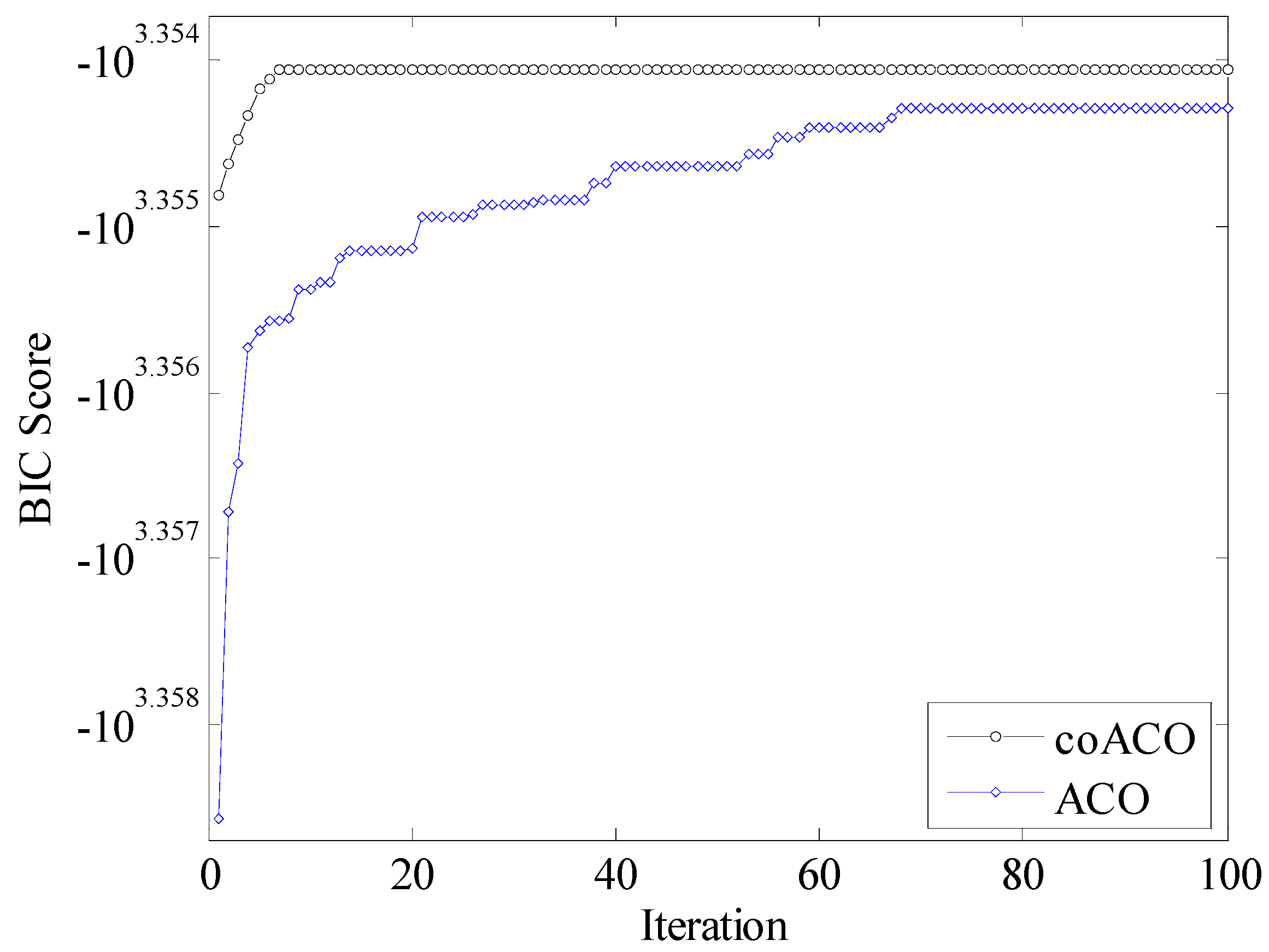
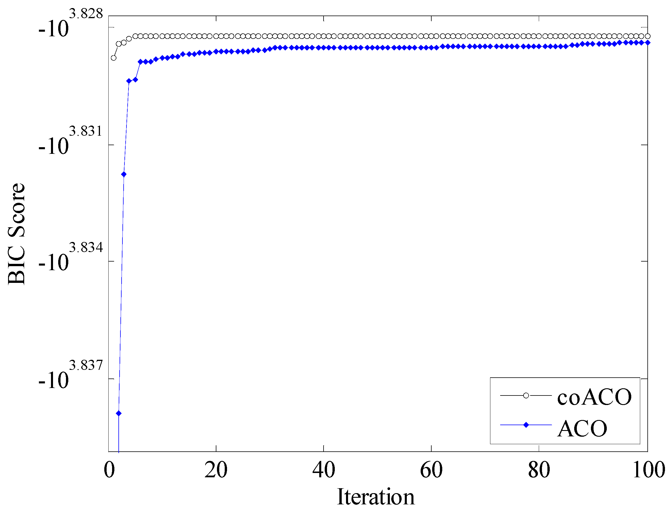
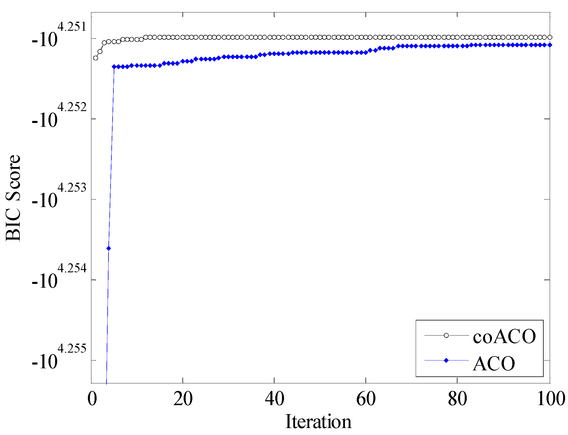
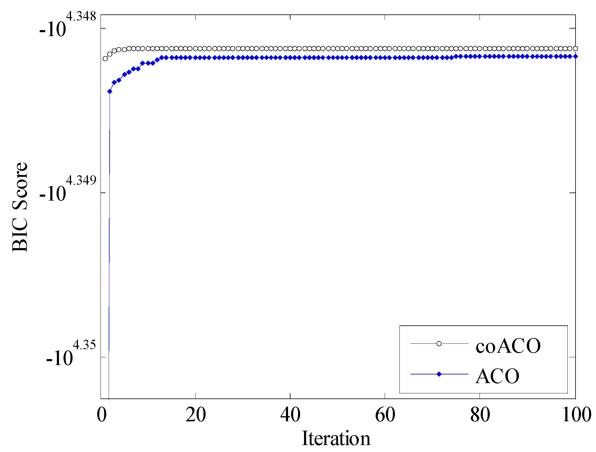
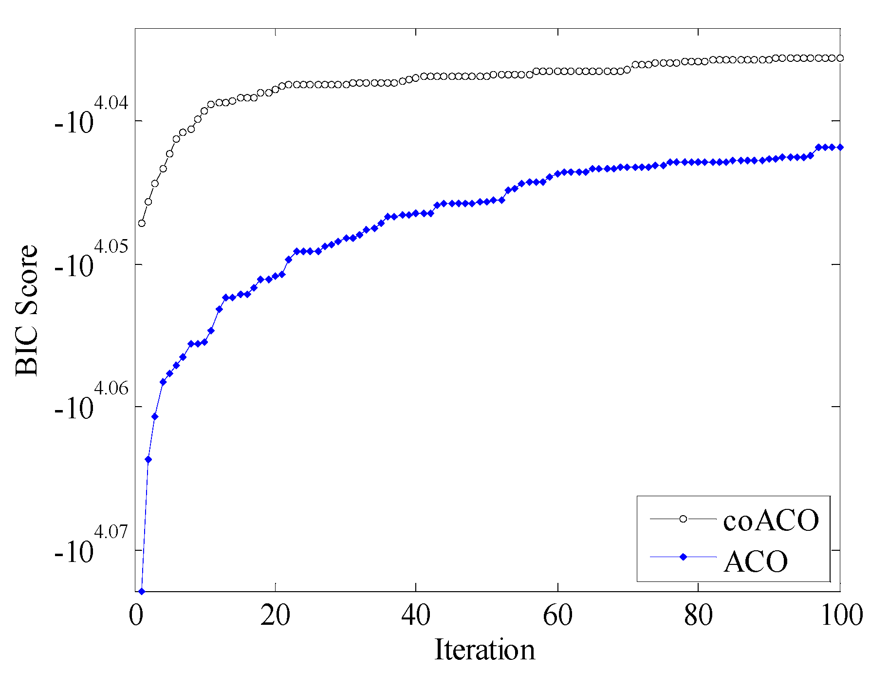
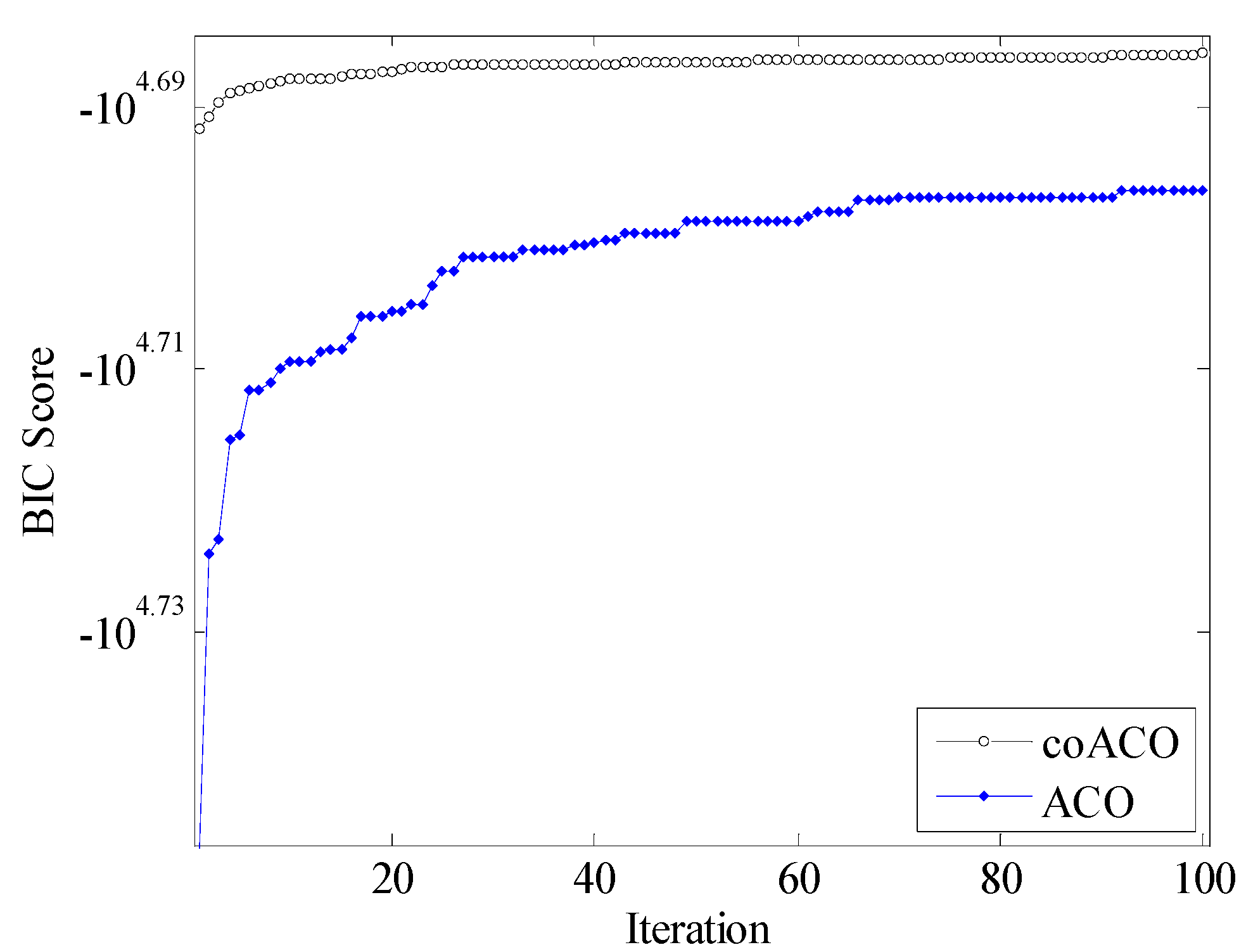
We run the stochastic algorithms, including ACO, coACO, and K2, 20 times independently for each dataset. The statistical results of the multiple independent experiments are listed in Table 2 for comparison, where six indicators are used to estimate the performances of the four algorithms, including the maximum/best, mean, median values, and the standard deviation of the BIC scores of the best networks obtained in each run. The last column, success rate (SR), is defined to represent the percentage of all 20 runs to obtain the BIC score that is not less than the corresponding original score listed in Table 1. It can be seen from Table 2 that coACO can always find the better BIC score for each dataset. It means that coACO can achieve a more efficient and robust performance than the basic ACO algorithm in learning the BN structure. The average evolution curves of the 20 independent tests on each dataset are illustrated in Figure 4, Figure 5, Figure 6, Figure 7, Figure 8, Figure 9 and Figure 10, which show the validity and rapid convergence of the proposed coACO algorithm.
Table 3 also shows the summary of the statistical results for various methods tested in the experiment, where μ ± σ denotes the mean and the standard deviation over the independent runs and the value inside (best) is the corresponding best value. The indicator It. is the smallest number of iterations when the algorithm finds the optimal network structure. The indicators A., D., and I. are used to denote the structure differences between the learned and the original network, namely, the number of arcs accidentally added (A.), deleted (D.), and inverted (I.), compared with the original network.
From the experimental results, it can be seen that, using the cooperative evolution strategies based on DE, the proposed coACO can greatly improve the performance of ACO in solving the BN structure-learning problem. As to the accuracy of the algorithms, coACO is superior to ACO for all test cases. This improvement is valid for not only BIC scores (see Table 2) but also the iteration number and the structural differences (see Table 3). As to the efficiency, the evolution curves shown in Figure 4, Figure 5, Figure 6, Figure 7, Figure 8, Figure 9 and Figure 10 show that coACO requires fewer computing iterations than the basic ACO. As to the robustness, coACO is also superior to the basic ACO, which can be deduced from the standard deviations of the independent runs shown in Table 2 and Table 3. The pheromone plays an important role in the solution-constructing process. The DE operations improve the capability of ants to accumulate the level of pheromone on arcs in the best structure. Due to the cooperative evolution characteristics, coACO can adjust the distribution of the pheromone trail to the best state in just a few iterations, and thus, yield the optimal network structure much faster. Though coACO employs some extra operators, it converged much faster. Therefore, coACO can obtain the best solution in a given small number of iterations.

5. Conclusions

This paper proposes coACO to improve the performance of the basic ACO in solving the BN structure-learning problem. The coACO divides the entire ant colony into several small ant groups and uses the pheromone as shared information and the cooperative factor. The cooperative evolution process of ant groups via collaborative interaction, which includes communicating pheromone information and sharing optimal networks between groups, can greatly improve the efficiency and accuracy. The coevolution mechanism based on DE is performed to lead the cooperative evolution process for all ant groups. DE operators can effectively adjust the cooperation information and lead all ant groups to evolve toward the optimum in a cooperative manner. Different from the widely used methodologies that combine ACO with constraint-based techniques, our work mainly focuses on improving the inherent search capability of ACO. Our algorithm employs the BIC metric as the scoring function; however, it is also applicable to other score metrics, such as K2 and MDL. Comparison test results show that our proposed coACO algorithm outperforms the ACO, K2, and B algorithms in terms of quality of the reconstructed BNs. Due to the coevolution characteristic, the coACO can adjust the pheromone distribution to the best state in just a few iterations, and thus yield the optimal network structure much faster. In a word, our developed coACO-based BN structure-learning algorithm is effective, accurate, efficient, and easy to implement. Our future work will apply the coACO to a more complex BN structure-learning problem in a real project with incomplete data.

Author Contributions

Conceptualization, X.Z.; Funding acquisition, S.J.; Project administration, S.J.; Software, X.L.; Writing—original draft, Y.X.; Writing—review & editing, X.Z.

Funding

This work is supported by the Beijing Municipal Education Commission, the National Natural Science Foundation of China (No. 61703012), and the Beijing Natural Science Foundation (No. 4182010).

Acknowledgments

The authors also gratefully acknowledge the helpful comments and suggestions of the reviewers, which help to improve the article.

Conflicts of Interest

The authors declare no conflict of interest.

References

  1. Pinto, P.C.; Nägele, A.; Dejori, M.; Runkler, T.A.; Sousa, J.M.C. Using a local discovery ant algorithm for Bayesian network structure learning. IEEE Trans. Evol. Comput. 2009, 13, 767–779. [Google Scholar] [CrossRef]
  2. Campos, L.M.; Fernández-Luna, J.M.; Gámez, J.A.; Puerta, J.M. Ant colony optimization for learning Bayesian networks. Int. J. Approx. Reason. 2002, 31, 291–311. [Google Scholar] [CrossRef]
  3. Larrañaga, P.; Karshenas, H.; Bielza, C.; Santana, R. A review on evolutionary algorithms in Bayesian network learning and inference tasks. Inf. Sci. 2013, 233, 109–125. [Google Scholar] [CrossRef]
  4. Gheisari, S.; Meybodi, M.R.; Dehghan, M.; Ebadzadeh, M.M. Bayesian network structure training based on a game of learning automata. Int. J. Mach. Learn. Cybern. 2017, 8, 1093–1105. [Google Scholar] [CrossRef]
  5. Martínez-Rodríguez, A.M.; May, J.H.; Vargas, L.G. An optimization-based approach for the design of Bayesian networks. Math. Comput. Model. 2008, 48, 1265–1278. [Google Scholar] [CrossRef]
  6. Cano, A.; Masegosa, A.R.; Moral, S.A. A method for integrating expert knowledge when learning Bayesian networks from data. IEEE Trans. Syst. Man Cybern. Part B Cybern. 2011, 41, 1382–1394. [Google Scholar] [CrossRef] [PubMed]
  7. Campos, L.M.; Castellano, J.G. Bayesian network learning algorithms using structural restrictions. Int. J. Approx. Reason. 2007, 45, 233–254. [Google Scholar] [CrossRef]
  8. Zhang, X.Y.; Jia, S.M.; Li, X.Z.; Guo, G. Learning the Bayesian networks structure based on ant colony optimization and differential evolution. In Proceedings of the 2018 4th International Conference on Control, Automation and Robotics (ICCAR), Auckland, New Zealand, 20–23 April 2018; pp. 354–358. [Google Scholar]
  9. Arefi, M.; Taheri, S.M. Possibilistic Bayesian inference based on fuzzy data. Int. J. Mach. Learn. Cybern. 2016, 7, 753–763. [Google Scholar] [CrossRef]
  10. Yan, L.J.; Cercone, N. Bayesian network modeling for evolutionary genetic structures. Comput. Math. Appl. 2010, 59, 2541–2551. [Google Scholar] [CrossRef]
  11. Khanteymoori, A.R.; Olyaee, M.-H.; Abbaszadeh, O.; Valian, M. A novel method for Bayesian networks structure learning based on Breeding Swarm algorithm. Soft Comput. 2017, 21, 6713–6738. [Google Scholar] [CrossRef]
  12. Wong, M.L.; Leung, K.S. An efficient data mining method for learning Bayesian networks using an evolutionary algorithm-based hybrid approach. IEEE Trans. Evol. Comput. 2004, 8, 378–404. [Google Scholar] [CrossRef]
  13. Wang, T.; Yang, J. A heuristic method for learning Bayesian networks using discrete particle swarm optimization. Knowl. Inf. Syst. 2010, 24, 269–281. [Google Scholar] [CrossRef]
  14. Ji, J.Z.; Zhang, H.X.; Hu, R.B. A Bayesian network learning algorithm based on independence test and ant colony optimization. Acta Autom. Sin. 2009, 35, 281–288. [Google Scholar] [CrossRef]
  15. Ji, J.Z.; Zhang, H.X.; Hu, R.B. A hybrid method for learning Bayesian networks based on ant colony optimization. Appl. Soft Comput. 2011, 11, 3373–3384. [Google Scholar] [CrossRef]
  16. Yang, J.; Li, L.; Wang, A.G. A partial correlation-based Bayesian network structure learning algorithm under linear SEM. Knowl. Based Syst. 2011, 24, 963–976. [Google Scholar] [CrossRef]
  17. Baumgartner, K.; Ferrari, S.; Palermo, G. Constructing Bayesian networks for criminal profiling from limited data. Knowl. Based Syst. 2008, 21, 563–572. [Google Scholar] [CrossRef]
  18. Garey, M.R.; Johnson, D.S. Computers and Intractability: A Guide to the Theory of NP-Completeness; WH Freeman Publishers: New York, NY, USA, 1979. [Google Scholar]
  19. Colorni, A.; Dorigo, M.; Maniezzo, V. Distributed optimization by ant colonies. In Proceedings of the First European Conference on Artificial Life, Paris, France, 11–13 December 1991; pp. 134–142. [Google Scholar]
  20. Dorigo, M.; Maniezzo, V.; Colorni, A. The ant system: Optimization by a colony of cooperating agents. IEEE Trans. Syst. Man Cybern. Part B Cybern. 1996, 26, 29–41. [Google Scholar] [CrossRef] [PubMed]
  21. Storn, R.; Price, K. Differential evolution: A simple and efficient heuristic for global optimization over continuous spaces. J. Glob. Optim. 1997, 11, 341–359. [Google Scholar] [CrossRef]
  22. Das, S.; Suganthan, P.N. Differential evolution: A survey of the state-of-the-art. IEEE Trans. Evol. Comput. 2011, 9, 4–31. [Google Scholar] [CrossRef]
  23. Derrac, J.; García, S.; Molina, D.; Herrera, F. A practical tutorial on the use of nonparametric statistical tests as a methodology for comparing evolutionary and swarm intelligence algorithms. Swarm Evol. Comput. 2011, 1, 3–18. [Google Scholar] [CrossRef]
  24. Duan, H.B.; Yu, Y.X.; Zhang, X.Y. Three-dimension path planning for UCAV using hybrid meta-heuristic ACO-DE algorithm. Simul. Model. Pract. Theory 2010, 18, 1104–1115. [Google Scholar] [CrossRef]
  25. Serani, A.; Leotardi, C.; Iemma, U.; Campana, E.F.; Fasano, G.; Diez, M. Parameter selection in synchronous and asynchronous deterministic particle swarm optimization for ship hydrodynamics problems. Appl. Soft Comput. 2016, 49, 313–334. [Google Scholar] [CrossRef] [Green Version]
  26. Zhang, X.Y.; Duan, H.B.; Yu, Y.X. Receding horizon control for multi-UAVs close formation control based on differential evolution. Sci. China Inf. Sci. 2010, 53, 223–235. [Google Scholar] [CrossRef]
  27. Zhang, X.Y.; Duan, H.B. An improved constrained differential evolution algorithm for unmanned aerial vehicle global route planning. Appl. Soft Comput. 2015, 26, 270–284. [Google Scholar] [CrossRef]
  28. Murphy, K. The Bayes Net Toolbox for Matlab. Comput. Sci. Stat. 2001, 33, 1024–1034. [Google Scholar]
Figure 1. The construction process of a BN.
Algorithms 11 00188 g001
Figure 2. The grouping operation and cooperative framework of coevolution ACO (coACO).
Algorithms 11 00188 g002
Figure 3. The crossover process of the pheromone matrix.
Algorithms 11 00188 g003
Figure 4. Evolution curves of the average Bayesian information criterion (BIC) score achieved by ACO and coACO on the ASIA dataset with n = 1000.
Algorithms 11 00188 g004
Figure 5. Evolution curves of the average BIC score achieved by ACO and coACO on the ASIA dataset with n = 3000.
Algorithms 11 00188 g005
Figure 6. Evolution curves of the average BIC score achieved by ACO and coACO on the ASIA dataset with n = 5000.
Algorithms 11 00188 g006
Figure 7. Evolution curves of the average BIC score achieved by ACO and coACO on the ASIA dataset with n = 8000.
Algorithms 11 00188 g007
Figure 8. Evolution curves of the average BIC score achieved by ACO and coACO on the ASIA dataset with n = 10,000.
Algorithms 11 00188 g008
Figure 9. Evolution curves of the average BIC score achieved by ACO and coACO on the ALARM dataset with n = 1000
Algorithms 11 00188 g009
Figure 10. Evolution curves of the average BIC score achieved by ACO and coACO on the ALARM dataset with n = 5000.
Algorithms 11 00188 g010
Table 1. A summary of the datasets used in the experiments.
NetworkNumber of CasesNodesArcsBIC Score
ASIA100088−2261.37
300088−6733.48
500088−11,194.67
800088−17,823.01
10,00088−22,290.78
ALARM10003746−11,156.05
50003746−48,593.10
Table 2. Statistical results of the BIC score for various methods.
NetworkNMethodBestMedianMeanWorstStd.SR (%)CPU Time (s)
ASIA1000coACO−2259.70−2259.70−2259.70−2259.700100116.826
ACO−2259.73−2259.73−2260.94−2262.761.5646074.335
K2−2267.64−2275.90−2276.53−2288.068.37600.118
B−2304.07----00.213
3000coACO−6733.48−6733.48−6733.48−6733.480100173.060
ACO−6733.48−6733.47−6736.14−6744.194.37660103.114
K2−6739.60−6755.06−6755.95−6797.7116.68800.142
B−6873.20----00.276
5000coACO−11,193.42−11,193.42−11,193.42−11,193.421.92 × 10−12100163.858
ACO−11,193.42−11,197.08−11,197.23−11,205.134.51240100.373
K2−11,197.08−11,218.39−11,224.51−11,300.6528.86700.174
B−11,450.81----00.288
8000coACO−17,823.01−17,823.01−17,823.01−17,823.010100203.835
ACO−17,823.01−17,823.01−17,826.72−17,837.125.77460127.463
K2−17,834.80−17,844.42−17,863.88−17,951.1338.80500.187
B−18,100.86----00.345
10,000coACO−22,290.78−22,290.78−22,290.78−22,290.783.83 × 10−12100246.144
ACO−22,290.78−22,294.73−22,293.15−22,294.732.04340153.925
K2−22,303.21−22,324.18−22,342.28−22,442.1742.48700.226s
B−22,572.73----00.459
ALARM1000coACO−10,818.45−10,852.26−10,852.26−10,950.4741.2561006481.540
ACO−10,957.50−11,002.89−11,012.03−11,138.5052.2341003687.500
K2−11,443.44−11,694.90−11699.26−11,993.50189.45003.285
B−3,425,441.5----07.913
5000coACO−48,501.03−48,517.21−48,525.78−48579.6428.65610010,800.721
ACO−49,341.99−49,661.63−49,701.69−50,329.43279.58906921.368
K2−50,968.63−51,949.21−51,858.65−52,867.42595.8604.867
B−5,425,441.5----025.681
SR, success rate.
Table 3. Statistical results for various methods (μ ± σ (best)).
NetworknMethodIt.A.D.I.
ASIA1000coACO6.4 ± 4.76 (1)0 ± 0 (0)1 ± 0 (1)1 ± 0 (1)
ACO43.8 ± 26.17 (4)0 ± 0 (0)1 ± 0 (1)1.9 ± 2.33 (0)
K2-0 ± 0 (0)2.5 ± 0.85 (1)4.40 ± 1.90 (2)
B-013
3000coACO2.7 ± 1.83 (1)0 ± 0 (0)0 ± 0 (0)1 ± 0 (1)
ACO47.9 ± 39.02 (2)0 ± 0 (0)0 ± 0 (0)3.3 ± 2.95 (1)
K2-0 ± 0 (0)1.3 ± 0.68 (0)4.6 ± 0.84 (3)
B-007
5000coACO4.9 ± 3.87 (1)0 ± 0 (0)1 ± 0 (1)0 ± 0 (0)
ACO42.2 ± 22.58 (11)0 ± 0 (0)1 ± 0 (1)2.9 ± 2.88 (0)
K2-0 ± 0 (0)2.2 ± 0.79 (1)4.8 ± 1.48 (3)
B-013
8000coACO6.2 ± 4.00 (2)0 ± 0 (0)0 ± 0 (0)1 ± 0 (1)
ACO52.1 ± 31.88 (5)0 ± 0 (0)0 ± 0 (0)3.5 ± 3.27 (1)
K2-0 ± 0 (0)0.9 ± 0.57 (0)5.3 ± 2.11 (2)
B-004
10,000coACO4.6 ± 3.60 (1)0 ± 0 (0)0 ± 0 (0)0 ± 0 (0)
ACO20.5 ± 21.74 (1)0 ± 0 (0)0 ± 0 (0)3.2 ± 2.15 (0)
K2-0 ± 0 (0)0.9 ± 0.57 (0)5.5 ± 2.64 (2)
B-008
ALARM1000coACO64.7 ± 13.12 (17)0 ± 0 (0)5.2 ±1.62 (4)12.7 ± 3.53 (9)
ACO81.8 ± 25.02 (57)0 ± 0 (0)9.2 ±1.69 (6)20.8 ± 5.03 (14)
K2-0 ± 0 (0)15.6 ± 2.55 (13)22.6 ± 4.25 (17)
B-0642
5000coACO81.1 ± 15.82 (46)0 ± 0 (0)1.2 ± 0.42 (1)14.6 ± 2.99 (10)
ACO58.5 ± 22.27 (20)0 ± 0 (0)5.4 ± 1.429 (3)58.5 ± 22.27 (20)
K2-0 ± 0 (0)10.1 ± 1.969 (7)33.4 ± 3.84 (26)
B-0197