High-Gain Observer-Based Sliding-Mode Dynamic Surface Control for Particleboard Glue Mixing and Dosing System

Abstract

In the process of particleboard glue mixing and dosing control under the working condition of intermediate frequency, a sliding-mode dynamic surface control strategy based on high-gain observer is proposed in this paper to deal with the problem of glue flow stability caused by strong nonlinearity. The high-gain observer (HGO) is aimed at estimating the derivative of the immeasurable system input signal for feedback, and the robustness of the system is improved by the dynamic surface control (DSC) method. Furthermore, the sliding-mode control (SMC) method is used to deal with disturbances caused by the uncertainties as well as external disturbances. It is proven that the system is exponential asymptotic stable by constructing a suitable Lyapunov function. Simulation results show that the proposed control methods can make the system track the expected flow value quickly and accurately. Finally, numerical simulation results are exhibited to authenticate and validate the effectiveness of the proposed control scheme.

1. Introduction

Particleboard is one of the three main products of wood-based panel [1]. If it can be utilized instead of log material, the shortage of wood resources can be alleviated to some extent, which is of great significance for the protection of ecological environment.

In the process of particleboard production, one of the main steps is glue mixing and dosing, which determines the technical level of particleboard production [2]. It is the mark of excellent mixing and dosing technology that the material can be accurately and proportionally matched according to the formula requirements. Excessive amount of glue will produce high moisture content particleboard, resulting in the bubble phenomenon, which will affect the yield, increase production capital, and result in an increase in formaldehyde emission. If the quantity of glue is too low, it will reduce the plasticity of the particleboard and make it difficult to compact. Meanwhile, physical properties such as static strength and plane tensile strength of particleboard will also decrease, which will affect the quality of the product. Therefore, the control of glue flow in particleboard glue mixing and dosing system plays a decisive role in the quality of the finished board.

At present, most of the wood-based panel production enterprises are dependent on artificial experience to control production, with proportional-integral-derivative (PID) as the primary control method used. The PID control strategy is widely applied in engineering [3,4,5,6]. However, this control strategy is not suitable for engineering control with high accuracy due to its poor dynamic performance, low anti-disturbance ability, and low control precision. To effectively solve the problem of tracking and anti-interference, the backstepping control method has been proposed by decomposing the high-order system into a series of low-order systems for the nonlinear system model with uncertainty [7,8,9,10,11]. The authors of Reference [7] designed an output feedback controller by combining backstepping and adaptive methods to deal with the synthesis of speed and flux for an induction motor drive. For the problem of a sensorless speed control for interior permanent magnet synchronous motors, Reference [8] outlined a nonlinear control based on the backstepping algorithm to improve robustness. Reference [9] proposed a novel gain-tuning method based on backstepping for variable PID controller. In this method, when system dynamics rapidly changes due to unknown disturbances, the system performance is robust and effective using the controller. For the problem of fault-tolerant control for a class of uncertain nonlinear system with actuator faults, the authors of Reference [10] used the backstepping approach to remove the classical assumption that the time derivative of output error should be known. Reference [11] applied backstepping to the Lagrangian form of the dynamics for quadrotor controller design to deal with unmodeled state-dependent disturbances. Though backstepping can solve nonlinear problems effectively, the traditional method requires repeated differentiation of virtual controller, and the control complexity increases rapidly with the increase in system order. The problem can be solved with the dynamic surface control (DSC) method proposed by Swaroop [12]. This method has been widely applied in the field of flight vehicles [13,14], unmanned aerial vehicles (UAV) [15], and missiles [16,17]. However, although DSC has some robustness and adaptability, it is not sufficient to achieve good control effect by its own robustness.

To improve the robust stability and transient performance of control systems, sliding-mode control (SMC) has been studied by many scholars to solve the problem of nonlinear systems [18,19,20,21,22]. To enhance robustness against parameter variations and disturbances, two model-free control system structures that include sliding-mode control were proposed and verified by real-time experimental results related to the position control of laboratory equipment represented by the twin rotor aerodynamic system in Reference [18]. In Reference [19], adaptive second-order sliding-mode control strategies were presented for a class of uncertain systems with unknown uncertainty bound. The authors adjusted the amplitude of the control law to control the uncertainties, enhanced the realization of second-order sliding mode, and made the state variables of the auxiliary system converge near the origin in finite time. In Reference [20], time-varying and constant switching frequency-based sliding-mode control methods were proposed for three-phase transformerless dynamic voltage restorers. The authors of Reference [21] proposed a new adaptive fuzzy sliding-mode control (AFSMC) design strategy for the control of a special class of three-dimensional fractional order chaotic systems with uncertainties and external disturbance and showed the efficiency of the proposed fractional adaptive controllers. Although SMC has strong robustness to parameter perturbation and external disturbance, it is worth noting that the above control methods are all based on measuring the speed and acceleration of signals, and the accuracy of measurement is vital for control results. However, in practical engineering, the measurement process has a certain degree of difficulty and the economic cost of the process is higher; therefore, the control method still has some limitations and challenges in practical situations.

To solve these problems, some scholars have proposed a high-gain observer (HGO) control strategy [23,24,25,26,27]. In Reference [23], an adaptive HGO was established to estimate the unmeasured states for the output-feedback control problem of a class of nonlinear large-scale system. In Reference [24], a decentralized control algorithm was developed based on HGO theory and fuzzy adaptive control algorithm for second-order uncertain nonlinear multiagent systems. In Reference [25], Mercorelli presented a sensorless control based on a HGO to reduce the effects of uncertainties on the electromagnetic valve actuator model and unmeasurable external disturbances. To solve the problem of single-rod electro-hydraulic servo having only one measured output state, a nonlinear backstepping control method based on a HGO was proposed to estimate the full state used by backstepping controllers in Reference [26]. The authors of Reference [27] proved that the extended HGO can be used to reduce the effect of disturbances while estimating and canceling the disturbance in one link of an underactuated system. Some scholars have combined SMC with HGO to achieve a better control effect. In Reference [28], a method was proposed for a flexible joint robotic arm, which used a high-gain observer with multiple sliding modes to ensure the observability of fault/unknown input signals, and sliding modes were utilized for their reconstruction. Reference [29] focused on the design of a high-gain observer that estimated the unmeasured states to get the knowledge of all state variables for sliding-mode controller in order to control tracking position and pressure.

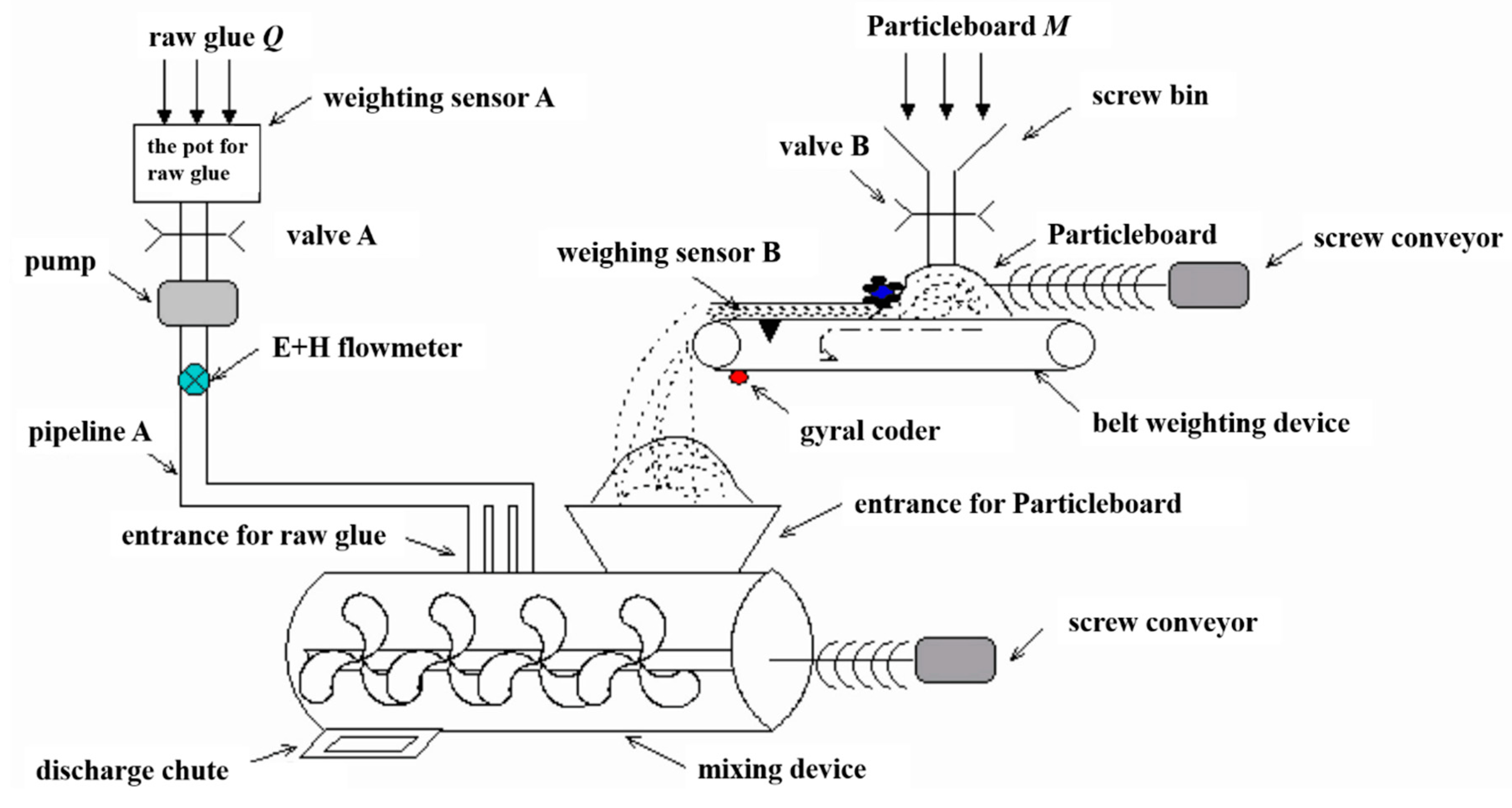
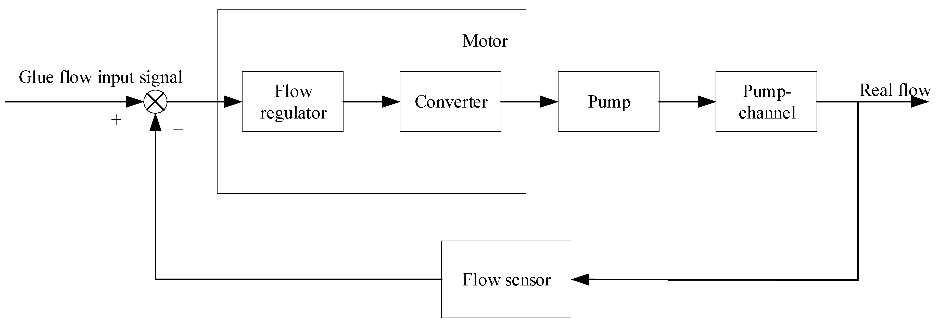
In the particleboard glue mixing and dosing system, the technical requirements differ with the thickness of the particleboard. When the thickness of the particleboard changes, the flow of the particleboard and gluing also changes. Meanwhile, the frequency of the system input can be adjusted to change the speed of the motor, and the speed of the dosing can be controlled to accurately control the dosing of the glue. In the intermediate frequency operation of particleboard mixing and dosing (30 Hz input excitation), there is a large nonlinearity that is influenced by two factors: The first is the influence of pipeline pressure and the second is the actuator and sensor entering the nonlinear region (saturation or dead zone) under this condition.

This paper was motivated by the SMC, DSC, and HGO methods to follow the desired glue flow. The main contributions of this paper can be summarized as follows:

(1) The equation of the state of particleboard mixing and dosing system was established in accordance with the intermediate frequency condition, and the structural parameters were identified using genetic factor recursive least-squares algorithm. A model that can reflect the lag and inertia characteristics of particleboard mixing and dosing process was established.

(2) A controller based on SMC and DSC was used to improve the response speed and the robustness of external noise disturbance. In addition, the HGO applied in combination with compound controller was designed, and the simulation results were compared.

(3) The appropriate Lyapunov functions were constructed to prove that all signals of the closed-loop system were semi-globally uniformly ultimately bounded and that the tracking error converged to zero asymptotically. Moreover, the benefits of the proposed control methods were authenticated and validated via simulation studies.

The paper is organized as follows: In Section 2, the particleboard glue mixing and dosing system under intermediate frequency operation is described. Section 3 introduces the sliding-mode dynamic surface control based on HGO schemes, and the closed system is proven to be semi-globally uniformly ultimately bounded. Simulation results of applying the proposed control methods to particleboard glue mixing and dosing system are shown in Section 4 to verify the effectiveness of the approach. Section 5 concludes the paper.

2. Process and System Description

2.1. Process of Particleboard Glue Mixing and Dosing System

The structure of particleboard glue mixing and dosing system is shown in Figure 1. It is composed of a particleboard-supported device, a glue-supported device, and a mixing device. The particleboard-supported device supports the whole system of the particleboard, consisting of the conveyor chute and the belt weighing device. The screw conveyor is used to send the particleboard to the discharge chute, the weighting sensor is employed to measure the particleboard’s weight, and the gyral coder is utilized to measure the rotating speed of the belt weighing device. The glue-supported device is constructed with the glue control pump and the E+H flowmeter, and the glue and particleboard are mixed by the mixing device.

In the process of dosing the particleboard, the particleboard is transported through the screw bin and valve B to the mixing device by the screw conveyor and belt weighing device. The control system collects the instantaneous weighing signal of the particleboard through weighing sensor B on the weighing conveyor belt. In the process of particleboard transportation, the corresponding instantaneous glue weight is calculated according to the amount of glue input. Then, according to the relationship between the rotating speed and the output of the pump, the speed is calculated.

2.2. System Description

The basic structure of a more common closed-loop control system for particleboard mixing and dosing is shown in Figure 2. The obtained actual flow by the flow sensor is compared with the input value, and the error is sent to the controller. To minimize the error, the controller constantly adjusts the frequency of the converter to change the speed of the squirrel-cage motor. In this way, the controlled supply by the glue pump results in steady supply of glue.

In this paper, the dynamics of the electrical components of the linear motor XY table have been ignored, and its velocity model can be expressed as a first-order differential equation for each axis [30].

$$v_i+\frac{b_i}{m_i}{v}_i+\frac{F_{Coul,i}}{m_i}sign(v_i)=\frac{k_i}{m_i}{u}_i$$

(1)

where $v_i$ is velocity; $m_i$ is mass; $b_i$ is viscous damping; $k_i$ is input gain, $F_{Coul,i}$ is coulomb friction and $i=x$, $y$, respectively.

The mathematical model of a simple and practical variable frequency pressure regulating system that supplies glue is derived for engineering, and when the voltage and frequency ratio of the power supply of squirrel-cage motors remain unchanged, its small deviation linear model is as follows [31]:

$$J\dot{\omega }=-(D+p{K}_0)\omega +p{K}_0{\omega }_1-pm$$

(2)

$$K_0=\frac{p}{r_2}{(\frac{V_{10}}{{\omega }_{10}})}^2$$

(3)

where ${\omega }_1$, $\omega$ are the deviations of stator power frequency and rotor electric angular velocity, respectively; $V_{10}$, ${\omega }_{10}$ are the value on static work point of voltage and frequency of the stator power supply, respectively; $p$ is role pair number; $r_2$ is the rotor resistance converted to stator side; $D$ is friction coefficient; $m$ is the deviation of load torque.

For the pump load, the torque is proportional to the square of the rotational speed, and the relationship of the deviations is as shown in Equation (4) when linearized by the small deviation.

$$m=K_m\omega$$

(4)

where $K_m$ is a constant. Invoking Equations (3) and (2), we get the following:

$$J\dot{\omega }=-(D+p{K}_0+K_m)\omega +p{K}_0{\omega }_1$$

(5)

Converted to transfer function, it can be represented as follows:

$$\frac{\omega (s)}{{\omega }_1(s)}=\frac{K_d}{1+T_{d}s}$$

(6)

where $T_d=(D+p(K_0+K_m))/J$, $K_d=p{K}_0/J$.

The mathematical model of the “pump channel” part is a set of partial differential equations. We can get the glue flow response curve of this link by a test method. The curve is fitted with an appropriate linear link, which can be described with the following transfer function:

$$\frac{\omega (s)}{{\omega }_1(s)}=\frac{K_d}{1+T_{d}s}$$

(7)

where $h$ is flow deviation; $T_b$ is time constant on the glue inertia; $K_b$ is a constant; $K_g$ is the differential coefficient of the liquid “anti-regulation” role.

According to the load characteristics, if we set appropriate parameters, such as acceleration and deceleration time, the curve can be set up to make its speed gradient less than flywheel torque of the motor driving system. For the pump load, the linear mode or half S mode can be used for the acceleration and deceleration curve. As the frequency response of the converter itself is very fast, a large integrator must be designed to weaken the influence of water hammer on the control signal when it is changed. This is done to enable the output frequency to change slowly into the new value. Therefore, the frequency converter is described with the following inertia:

$$\frac{{\omega }_1(s)}{u(s)}=\frac{K_{v}s}{1+T_{v}s}$$

(8)

where $u$ is control signal deviation; $K_v$ and $T_v$ are constants; $T_v$ can be set by the user over a considerable range.

The PI regulator is used by most flow regulators, and its transfer function is as follows:

$$\frac{u(s)}{e(s)}=\frac{1+K_{t}s}{T_{t}s}$$

(9)

where $e$ is error signal; $K_t$ and $T_t$ are the regulator parameter.

If $T_v\ge \max \left\{T_a,T_b\right\}$, the mathematical model of the “motor pump channel” part can be merged into one link based on the model reduction theory according to Equations (6) and (7):

$$\frac{h(s)}{{\omega }_1(s)}=\frac{K_d(K_b-K_g)s}{1+(T_d+T_b)s}$$

(10)

According to the Equations (8), (9), and (10), the following can be obtained:

$$\frac{h(s)}{e(s)}=\frac{K_v{K}_d(1+K_{t}s)(K_b-K_g)s}{T_{t}s(1+T_{v}s)[1+(T_d+T_b)s]}$$

(11)

Therefore, the open loop transfer function of the system can be simplified:

$$\frac{h(s)}{e(s)}=\frac{K_v{K}_d(1+K_{t}s)(K_b-K_g)}{T_t(1+T_{v}s)[1+(T_d+T_b)s]}$$

(12)

Data collection was carried out on the mixing and dosing device of GM&D-A type particleboard in the laboratory. When the output of the glue flow was stable, the off-line data of the whole process were recorded with the system input of 30 Hz excitation signal. The model parameters were identified using recursive least-square algorithm based on genetic factor. The model was a four-order system with lagging terms, and the fitting degree was 93.32. The simplified model structure is as follows:

$$\frac{k(1+T_{1}s)}{s(1+T_{2}s)(1+T_{3}s)(1+T_{4}s)}$$

(13)

where the result of parameter identification $k=5.668e-005$, $T_1=-72.1897$, $T_2=3.5079$, $T_3=-0.76099$, $T_4=-1.3186$, $\tau =2.6523$. The transfer function is as follows:

$$\frac{(-0.001142s+1.581e^{-0.005})e^{-2.65s}}{s^4+2.358s^3+1.587s^2+0.2841s}$$

(14)

where the simplified state equation can be given as follows:

$$\{\begin{array}{l}{\dot{x}}_1=x_2\\ {\dot{x}}_2=x_3\\ {\dot{x}}_3=-0.284x_1-1.587x_2-2.358x_3+0.02899u\\ y=x_1\end{array}$$

(15)

which is the nominal system of the particleboard glue mixing and dosing system. In practical engineering, the change of pressure for the glue flow and the flow rate will be affected under the intermediate frequency condition, which makes the particleboard glue mixing and dosing system suffer more external disturbances. Therefore, we changed the model represented in Equation (15) as follows:

$$\{\begin{array}{l}{\dot{x}}_1=x_2\\ {\dot{x}}_2=x_3\\ {\dot{x}}_3=f(x)+gu+D\\ y=x_1\end{array}$$

(16)

where $f(x)=-0.284x_1-1.587x_2-2.358x_3$, $u$ is control input and $y$ is the control output, $g=0.02899$, $D=\Delta f+d$ is expressed as the compound disturbance, which includes the uncertainty of parameter identification $\Delta f$ and the nonlinear external disturbances $d$.

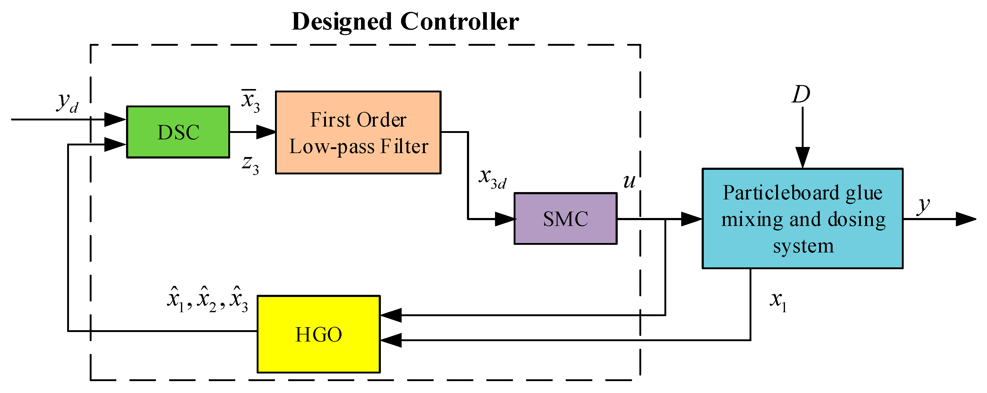
3. Design of High-Gain Observer-Based Sliding-Mode Dynamic Surface Controller

In this section, we design a compound control strategy for particleboard glue mixing and dosing system with the intermediate frequency condition. A high-gain observer-based sliding-mode dynamic surface controller will be designed. To estimate the derivative of the system input signal for the feedback to the controller, HGO is used, with $x_1$ as the input. Then, the output of the observer ${\widehat{x}}_1$, ${\widehat{x}}_2$, and ${\widehat{x}}_3$ is put into the compound controller instead of $x_1$, $x_2$, and $x_3$. The controller is used to deal with nonlinear disturbance, and the configuration is shown in Figure 3.

To design the controller, we need to make the following assumptions:

Assumption 1.

The input signal $y=x_1$ and its derivative exist and are bounded.

Assumption 2.

$D$ is bounded and the boundary is unknown., i.e., $\left|D\right|<\mathsf{\Phi }$.

3.1. Designs of High-Gain Observer

To estimate the derivative of the system input signal for feedback to the controller, high-gain observer is used. $x_1$ is the input into the high-gain observer, and the output of the observer ${\widehat{x}}_1$, ${\widehat{x}}_2$, and ${\widehat{x}}_3$ is put into the controller instead of $x_1$, $x_2$, and $x_3$.

To analyze the convergence of observer, the system model given in Equation (16) is considered:

$$\{\begin{array}{l}{\dot{x}}_1=x_2\\ {\dot{x}}_2=x_3\\ {\dot{x}}_3=F(x,u,D)\\ y=x_1\end{array}$$

(17)

where $F(x,u,D)=f(x)+0.02899u+D$, satisfying Lipschitz condition.

The high-gain observer is designed as follows:

$$\{\begin{array}{l}{\dot{\widehat{x}}}_1={\widehat{x}}_2+h_1(y-{\widehat{x}}_1)\\ {\dot{\widehat{x}}}_2={\widehat{x}}_3+h_2(y-{\widehat{x}}_1)\\ {\dot{\widehat{x}}}_3=F(\widehat{x},u)+h_3(y-{\widehat{x}}_1)\end{array}$$

(18)

where $\widehat{F}(\widehat{x},u)$ is the nominal model of $F(x,u,D)$.

Defining observation error $\tilde{x}=\left[\begin{array}{l}{\tilde{x}}_1\\ {\tilde{x}}_2\\ {\tilde{x}}_3\end{array}\right]=\left[\begin{array}{l}{x}_1-{\widehat{x}}_1\\ x_2-{\widehat{x}}_2\\ x_3-{\widehat{x}}_3\end{array}\right]$, considering (17) and (18), we know that

$$\{\begin{array}{l}{\dot{\tilde{x}}}_1=-h_1{\tilde{x}}_1+{\tilde{x}}_2\\ {\dot{\tilde{x}}}_2=-h_2{\tilde{x}}_1+{\tilde{x}}_3\\ {\dot{\tilde{x}}}_3=-h_3{\tilde{x}}_1+\delta (x,\tilde{x},d)\end{array}$$

(19)

where $\delta (x,\tilde{x},D)=F(x,u,D)-\widehat{F}(\widehat{x},u)$ is modeling uncertainty.

Equation (17) can be written as follows:

$$\dot{\tilde{x}}=A\tilde{x}+\left[\begin{array}{l}0\\ 0\\ \delta \end{array}\right]$$

(20)

where $A=\left[\begin{array}{lll}-h_1& 1& 0\\ -h_2& 0& 1\\ -h_3& 0& 0\end{array}\right]$, $\tilde{x}=\left[\begin{array}{l}{\tilde{x}}_1\\ {\tilde{x}}_2\\ {\tilde{x}}_3\end{array}\right]$

When $\delta$ is not considered, the eigenvalue is negative if $A$ is Hurwitz. Then, the observation $\tilde{x}$ is asymptotically convergent. Therefore, we need to choose the suitable $h_1$, $h_2$, and $h_3$ to make $A$ satisfy Hurwitz.

As for the effect of $\delta$ on $\tilde{x}$, from Equation (19), it can be written as follows:

$$\{\begin{array}{l}s{\tilde{x}}_1=-h_1{\tilde{x}}_1+{\tilde{x}}_2\\ s{\tilde{x}}_2=-h_2{\tilde{x}}_1+{\tilde{x}}_3\\ s{\tilde{x}}_3=-h_3{\tilde{x}}_1+\delta \end{array}$$

Therefore

$$\{\begin{array}{l}{\tilde{x}}_1=\delta /(s^3+h_1{s}^2+h_{2}s+h_3)\\ {\tilde{x}}_2={\tilde{x}}_1(s+h_1)\\ {\tilde{x}}_3={\tilde{x}}_1(s^2+h_{1}s+h_2)\end{array}$$

and we obtain the following transfer function:

$$\begin{array}{l}{G}_{10}(s)=\frac{{\tilde{x}}_1(s)}{\delta (s)}=\frac{1}{s^3+h_1{s}^2+h_{2}s+h_3}\\ G_{20}(s)=\frac{{\tilde{x}}_2(s)}{\delta (s)}=\frac{(s+h_1)}{s^3+h_1{s}^2+h_{2}s+h_3}\\ G_{30}(s)=\frac{{\tilde{x}}_3(s)}{\delta (s)}=\frac{(s^2+h_{1}s+h_2)}{s^3+h_1{s}^2+h_{2}s+h_3}\end{array}$$

From $G_{10}(s)$, $G_{20}(s)$, and $G_{30}(s)$, we can see the following:

$$A(G_{10}(j\omega ))=\left|\frac{1}{-{\omega }^{3}j-h_1{\omega }^2+h_2\omega j+h_3}\right|=\frac{1}{\sqrt{{(h_3-h_1{\omega }^2)}^2+{(h_2\omega -{\omega }^3)}^2}}$$

$$A(G_{20}(j\omega ))=\left|\frac{\omega j+h_1}{-{\omega }^{3}j-h_1{\omega }^2+h_2\omega j+h_3}\right|=\sqrt{\frac{{\omega }^2+h_1{}^2}{{(h_3-h_1{\omega }^2)}^2+{(h_2\omega -{\omega }^3)}^2}}$$

$$A(G_{20}(j\omega ))=\left|\frac{-{\omega }^2+h_1\omega j+h_2}{-{\omega }^{3}j-h_1{\omega }^2+h_2\omega j+h_3}\right|=\sqrt{\frac{{(h_2-{\omega }^2)}^2+h_1{}^2{\omega }^2}{{(h_3-h_1{\omega }^2)}^2+{(h_2\omega -{\omega }^3)}^2}}$$

To make ${\tilde{x}}_1\to 0$, ${\tilde{x}}_2\to 0$, ${\tilde{x}}_3\to 0$, $h_3\gg h_2\gg h_1\gg 1$ must be guaranteed.

We let

$$h_1=\frac{{\alpha }_1}{\epsilon },h_2=\frac{{\alpha }_2}{{\epsilon }^2},h_3=\frac{{\alpha }_3}{{\epsilon }^3}$$

(21)

where ${\alpha }_1$, ${\alpha }_2$ and ${\alpha }_3$ are real numbers, $\epsilon \ll 1$.

Therefore, the observer expression can be written as follows:

$$\{\begin{array}{l}{\dot{\widehat{x}}}_1={\widehat{x}}_2+\frac{{\alpha }_1}{\epsilon }\left(y-{\widehat{x}}_1\right)\\ {\dot{\widehat{x}}}_2={\widehat{x}}_3-\frac{{\alpha }_2}{{\epsilon }^2}\left(y-{\widehat{x}}_1\right)\\ {\dot{\widehat{x}}}_3=\widehat{F}(\widehat{x},u)-\frac{{\alpha }_3}{{\epsilon }^3}\left(y-{\widehat{x}}_1\right)\end{array}$$

(22)

If we put Equation (21) into $G_0(s)=\left[\begin{array}{l}{G}_{10}(s)\\ G_{20}(s)\\ G_{30}(s)\end{array}\right]$

$$G_0(s)=\frac{\epsilon }{{(\epsilon s)}^3+{\alpha }_1{(\epsilon s)}^2+{\alpha }_2\epsilon s+{\alpha }_3}\left[\begin{array}{c}{\epsilon }^2\\ {\epsilon }^{2}s+{\alpha }_1\epsilon \\ {(\epsilon s)}^2+{\alpha }_1\epsilon s+{\alpha }_2\end{array}\right]$$

where $\underset{\epsilon \to \infty }{\lim }{G}_0(s)=0$. Obviously, modeling uncertainty can be overcome by high gain.

3.2. Designs of Sliding-Mode Dynamic Surface Controller

For the system shown in Equation (16), the detailed design steps of the controller are as follows:

Step 1.

Define the error of the first surface:

$$z_1=x_1-y_d$$

(23)

where $y_d$ is the given tracking signal and its derivative is known.

The time derivative of $z_1$ is given as follows:

$${\dot{z}}_1=x_2-{\dot{y}}_d$$

(24)

To make $z_1$ converge to 0, design virtual control variable:

$${\overline{x}}_2=-c_1{z}_1+{\dot{y}}_d$$

(25)

where $c_1$ is the parameter to be designed.

Unlike the backstepping control method, put ${\overline{x}}_2$ into a low-pass first-order filter and get the output $x_{2d}$:

$$x_{2d}+{\tau }_2{\dot{x}}_{2d}={\overline{x}}_2$$

(26)

where ${\tau }_2$ is a time constant of the filter. The initial condition of Equation (26) is as follows:

$${\overline{x}}_2(0)=x_{2d}(0)$$

(27)

Step 2.

Define the error of the second surface:

$$z_2=x_2-x_{2d},$$

(28)

and its derivative is as follows:

$${\dot{z}}_2={\dot{x}}_2-{\dot{x}}_{2d}=x_3-{\dot{x}}_{2d}$$

(29)

To make Z₂ converge to 0, design virtual control variable:

$${\overline{x}}_3=-c_2{z}_2+{\dot{x}}_{2d}$$

(30)

where $c_2$ is design parameter.

Again, put ${\overline{x}}_3$ into a low-pass first-order filter and get the output $x_{3d}$:

$$x_{3d}+{\tau }_3{\dot{x}}_{3d}={\overline{x}}_3$$

(31)

where ${\tau }_3$ is a time constant of the filter. The initial condition of Equation (31) is as follows:

$${\overline{x}}_3(0)=x_{3d}(0)$$

(32)

Step 3.

Define the error of the third surface:

$$z_3=x_3-x_{3d}$$

(33)

and its derivative is as follows:

$${\dot{z}}_3={\dot{x}}_3-{\dot{x}}_{3d}=f(x)+gu+D-{\dot{x}}_{3d}$$

(34)

To make $z_3$ converge to 0, design the control law:

$$u=\frac{-c_3{z}_3-f(x)+{\dot{x}}_{3d}-\eta \mathrm{sgn}(z_3)}{g}$$

(35)

where $c_3$ is also the parameter to be designed. Due to $\left|D\right|\le \mathsf{\Phi }$, design $\eta \ge \mathsf{\Phi }$.

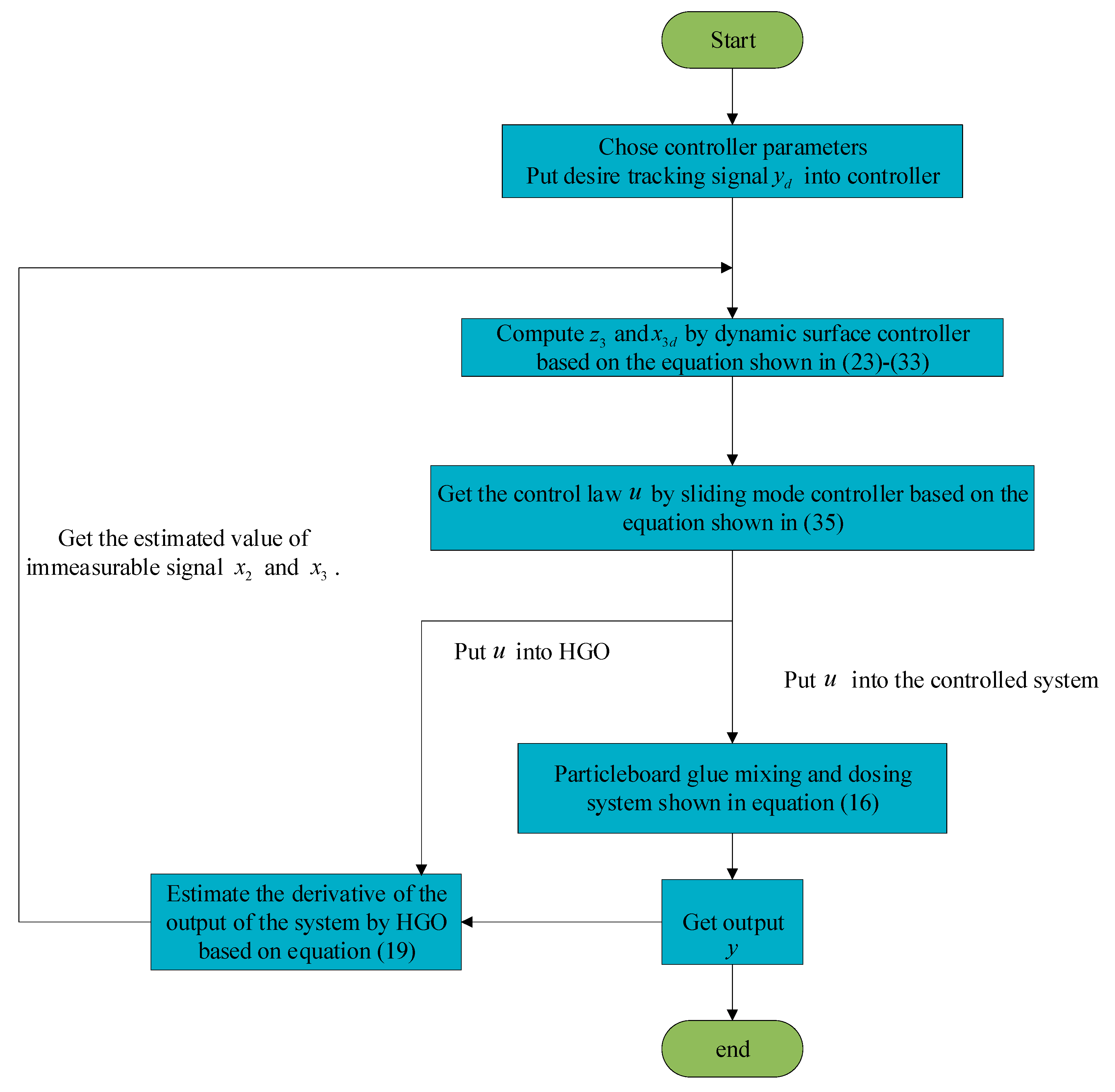
The flowchart of the proposed control algorithm is shown in Figure 4.

Define the filtering error $y_2$, $y_3$:

$$y_2=x_{2d}-{\overline{x}}_2, y_3=x_{3d}-{\overline{x}}_3$$

Considering position tracking, virtual control, and filtering error, define Lyapunov function:

$$V=\frac{1}{2}{z}_1^2+\frac{1}{2}{z}_2^2+\frac{1}{2}{z}_3^2+\frac{1}{2}{y}_2^2+\frac{1}{2}{y}_3^2$$

(36)

Differentiating Equation (36) with respect to time:

$$\begin{array}{lll}\dot{V}& =& z_1{\dot{z}}_1+z_2{\dot{z}}_2+z_3{\dot{z}}_3+y_2{\dot{y}}_2+y_3{\dot{y}}_3\\ & =& z_1(x_2-{\dot{y}}_d)+z_2(x_3-{\dot{x}}_{2d})+z_3(f(x)+gu+D-{\dot{x}}_{3d})\\ & & +y_2({\dot{x}}_{2d}-{\dot{\overline{x}}}_2)+y_3({\dot{x}}_{3d}-{\dot{\overline{x}}}_3)\end{array}$$

Invoking Equations (26), (28), (30), (33), and (35), we get the following:

$$\begin{array}{lll}\dot{V}& =& z_1(z_2+y_2-c_1{z}_1)+z_2(z_3+y_3-c_2{z}_2)-c_3{z}_3^2\\ & & +z_3(D-\eta \mathrm{sgn}(z_3))+y_2(T_2-\frac{y_2}{{\tau }_2})+y_3(T_3-\frac{y_3}{{\tau }_3})\\ & =& z_1(z_2+y_2)+z_2(z_3+y_3)-c_1{z}_1^2-c_2{z}_2^2-c_3{z}_3^2\\ & & +z_3(D-\eta \mathrm{sgn}(z_3))+y_2(T_2-\frac{y_2}{{\tau }_2})+y_3(T_3-\frac{y_3}{{\tau }_3})\\ & =& z_1(z_2+y_2)+z_2(z_3+y_3)-c_1{z}_1^2-c_2{z}_2^2-c_3{z}_3^2\\ & & +z_3(D-\eta \mathrm{sgn}(z_3))+y_2(T_2-\frac{y_2}{{\tau }_2})+y_3(T_3-\frac{y_3}{{\tau }_3})\end{array}$$

(37)

where

$$T_2=c_1(z_2+y_2-c_1{z}_1)-{\ddot{y}}_d$$

$$T_3=c_2(z_3+y_3-c_2{z}_2)-{\ddot{x}}_{2d}$$

are all bounded. Define the upper bound of them as $M_2$ and $M_3$, respectively, yielding $\frac{T_i^2}{M_i^2}-1\le 0\hspace{0.17em}(i=1,2)$.

Owing to $\eta \ge \mathsf{\Phi }$, $z_3(D-\eta \mathrm{sgn}(z_3))\le 0$. Then

$$\begin{array}{lll}\dot{V}& \le & \left|z_1\right|\left|z_2\right|+\left|z_1\right|\left|y_2\right|+\left|z_2\right|\left|z_3\right|+\left|z_2\right|\left|y_3\right|\\ & & -c_1{z}_1^2-c_2{z}_2^2-c_3{z}_3^2-\frac{y_2^2}{{\tau }_2}+\left|T_2\right|\left|y_2\right|-\frac{y_3^2}{{\tau }_3}+\left|T_3\right|\left|y_3\right|\\ & \le & \frac{1}{2}(z_1^2+z_2^2)+\frac{1}{2}(z_1^2+y_2^2)+\frac{1}{2}(z_2^2+z_3^2)\\ & & +\frac{1}{2}(z_2^2+y_3^2)-c_1{z}_1^2-c_2{z}_2^2-c_3{z}_3^2-\frac{y_2^2}{{\tau }_2}\\ & & +\frac{1}{2}(T_2^2{y}_2^2+1)-\frac{y_3^2}{{\tau }_3}+\frac{1}{2}(T_3^2{y}_3^2+1)\\ & =& 1+(1-c_1)z_1^2+(\frac{3}{2}-c_2)z_2^2+(\frac{1}{2}-c_3)z_3^2\\ & & +(\frac{1}{2}+\frac{1}{2}{T}_2^2-\frac{1}{{\tau }_2})y_2^2+(\frac{1}{2}+\frac{1}{2}{T}_3^2-\frac{1}{{\tau }_3})y_3^2\end{array}$$

Design the following parameters:

$$c_1\ge 1+\Delta , c_2\ge \frac{3}{2}+\Delta , c_3\ge \frac{1}{2}+\Delta$$

$$\frac{1}{{\tau }_2}\ge \frac{1}{2}{M}_2^2+\frac{1}{2}+\Delta , \frac{1}{{\tau }_3}\ge \frac{1}{2}{M}_3^2+\frac{1}{2}+\Delta$$

(38)

where $\Delta$ is a small positive real number:

$$\begin{array}{l}\dot{V}\le -\Delta (z_1^2+z_2^2+z_3^2)+y_2^2(\frac{1}{2}{T}_2^2-\frac{1}{2}{M}_2^2-\Delta )+y_3^2(\frac{1}{2}{T}_3^2-\frac{1}{2}{M}_3^2-\Delta )+1\\ \hspace{1em}=-2\Delta V+y_2^2\frac{M_2^2}{2}(\frac{T_2^2}{M_2^2}-1)+y_3^2\frac{M_3^2}{2}(\frac{T_3^2}{M_3^2}-1)+1\end{array}$$

Invoking Equation (38), we get the following:

$$\dot{V}\le -2\Delta V+1,$$

(39)

Let $\mathsf{\Omega }$ be one of the bound of $V$ and make $\Delta >\frac{1}{2\mathsf{\Omega }}$, so

$$\dot{V}\le -\frac{V}{\mathsf{\Omega }}+1\le 0$$

(40)

We get the solution of the above inequality [32]:

$$V\le \frac{1}{2\Delta }+(V(0)-\frac{1}{2\Delta })e^{-2\Delta t}$$

(41)

Through the above analysis, the closed-loop system is uniformly ultimately bounded and all the signals converge to zero by choosing the appropriate sliding-mode dynamic surface controller parameters $c_1$, $c_2$, $c_3$, ${\tau }_2$, and ${\tau }_3$.

4. Simulation Analysis

For particleboard glue mixing and dosing system, considering the stage of glue flow dosing, we carried out a simulation study to validate the effectiveness of the proposed strategy based on Matlab2016a/Simulink. In this simulation, the compound controller was designed according to Equations (22) and (35). Considering the disturbance caused by the pump, channel, and flow sensor, different forms of the disturbance was exerted on the system, and the simulation results were divided into two parts. To make the output signal of the system track the desired signal faster without overshoot, the following parameters of the observers were chosen:

$$\epsilon =0.01, {\alpha }_1={\alpha }_2=3, {\alpha }_3=1, c_1=c_2=c_3=10, {\tau }_2={\tau }_3=0.001, {\alpha }_1=4$$

As for the initial values of the HGO and the first-order low-pass filters:

$${\widehat{x}}_1(0)={\widehat{x}}_2(0)={\widehat{x}}_3(0)=0.5, x_{2d}(0)={\overline{x}}_2(0)=100, x_{3d}(0)={\overline{x}}_3(0)=1000$$

The desire glue flow $y_d=10 L/min$, $d=0.1sin4t+0.1cos6t$, $x_1\left(0\right)=x_2\left(0\right)=x_3\left(0\right)=0$. The simulation results are shown in Figure 5, Figure 6, Figure 7, Figure 8, Figure 9, Figure 10, Figure 11, Figure 12, Figure 13 and Figure 14. Next, the proposed controller was compared with PID and backstepping mode controllers.

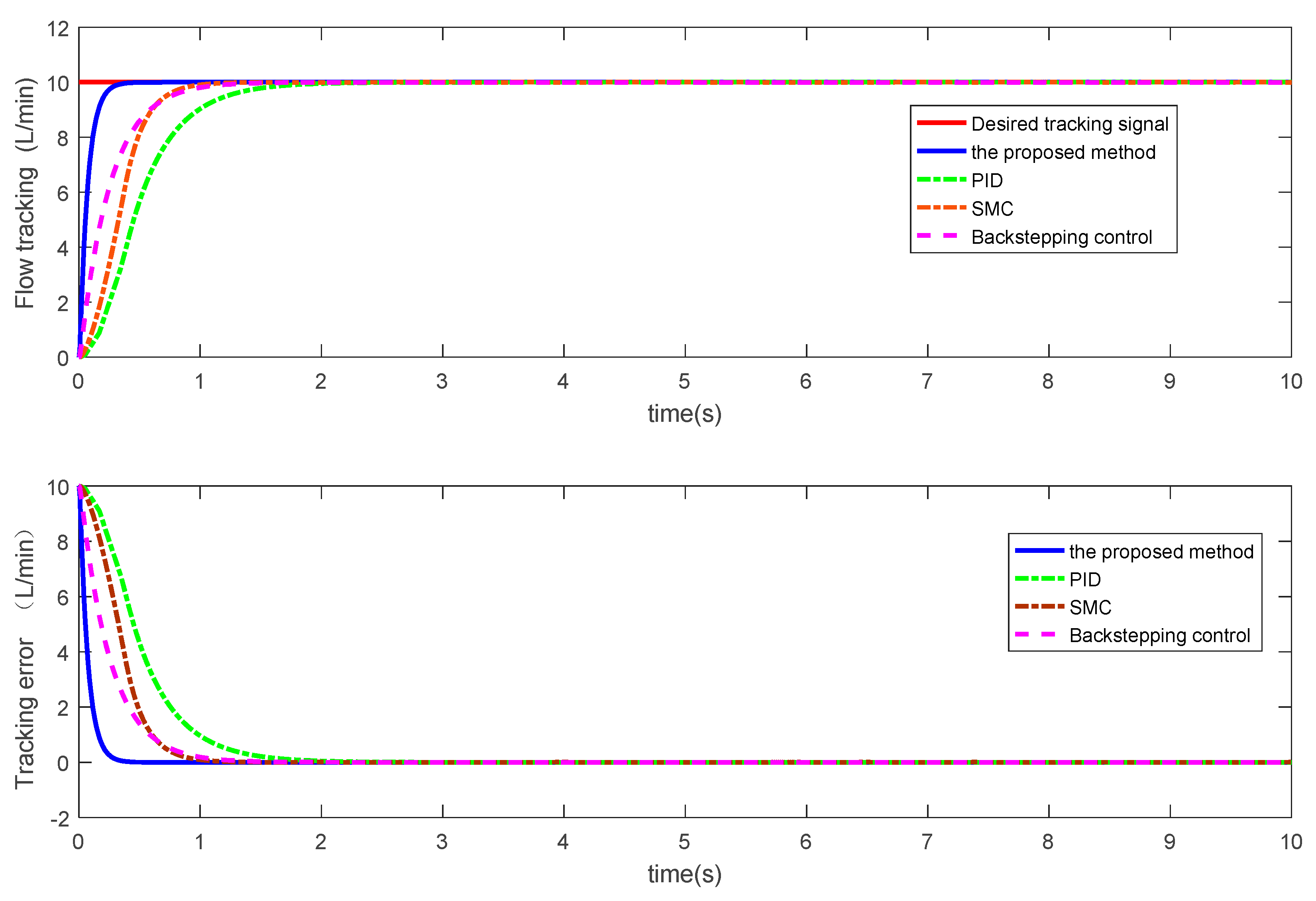
The time response of desired glue flow signal tracking and tracking error is shown in Figure 5. It can be seen that the proposed control method is much faster than traditional PID control and SMC approaches. It is also clear that the response speed of the proposed method is faster than the backstepping control based on SMC and can realize the quick, accurate, and non-overshoot positioning.

The time response of the first-order low-pass filter is shown in Figure 6. It can be seen that the virtual control variables almost coincide with the output variables of the filter, and it is clear that the accuracy of the derivative of virtual control is good with the output of the filter.

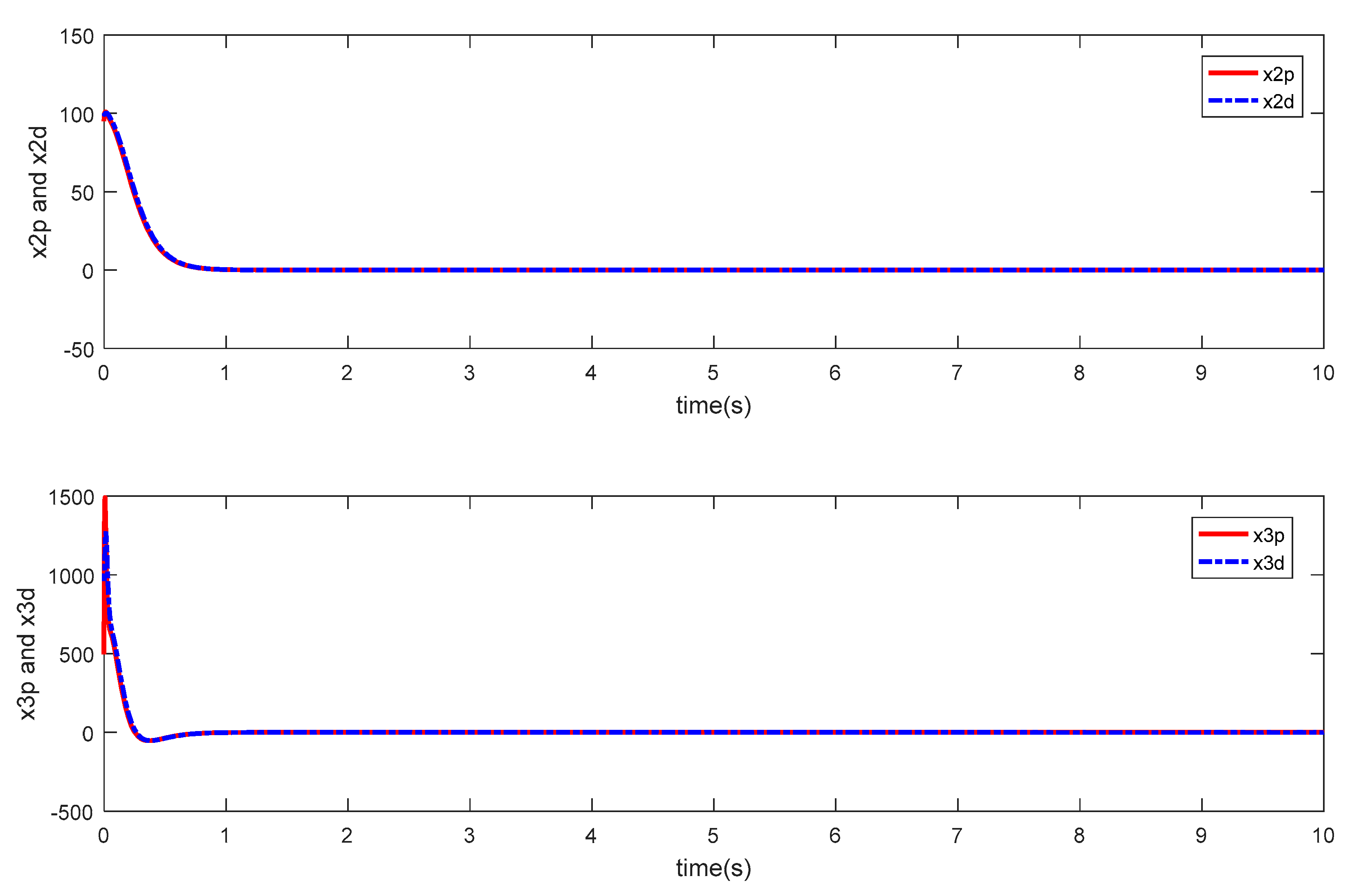
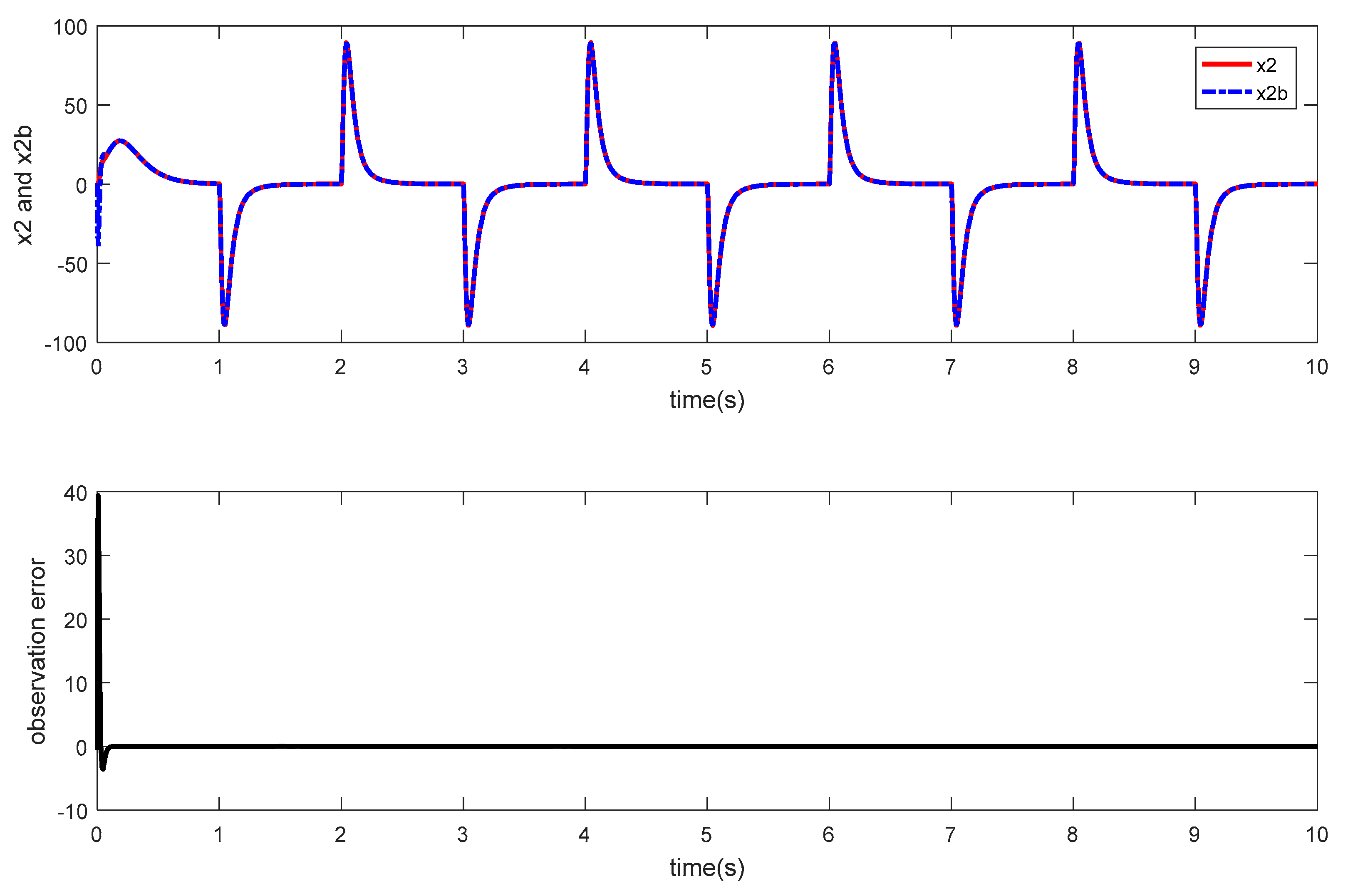
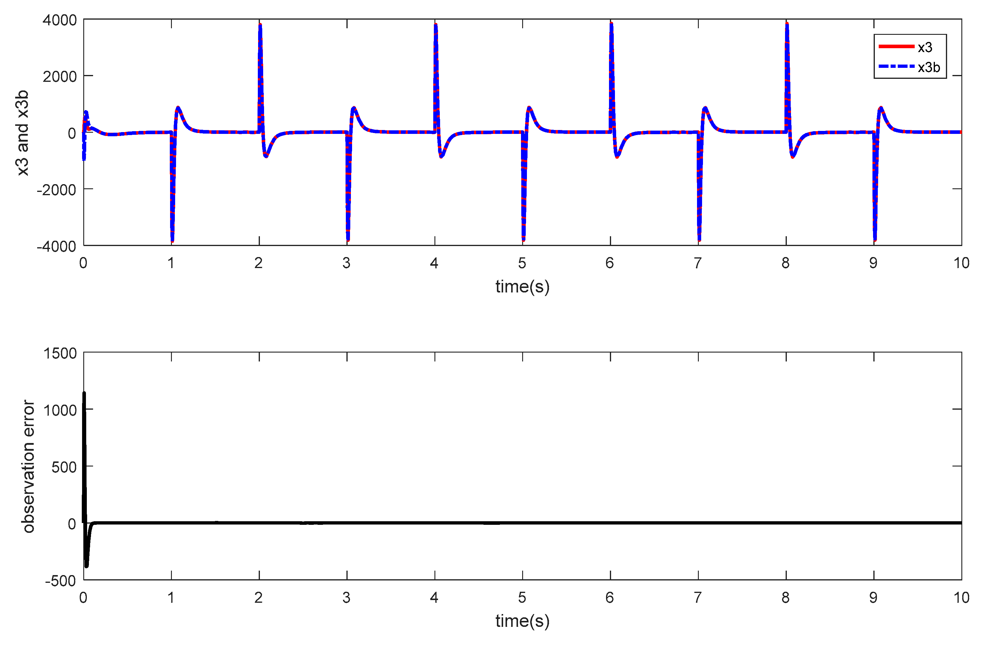
Comparisons of the actual and estimated values of the system input via HGO are shown in Figure 7 and Figure 8. ×2 and ×3 represent the actual system input, which cannot be measured in actual working conditions. ×2b and ×3b represent ${\widehat{x}}_2$ and ${\widehat{x}}_3$, respectively, namely the estimation of ×2 and ×3. It can be seen that the estimated values of HGO output can be a good substitute for system input.

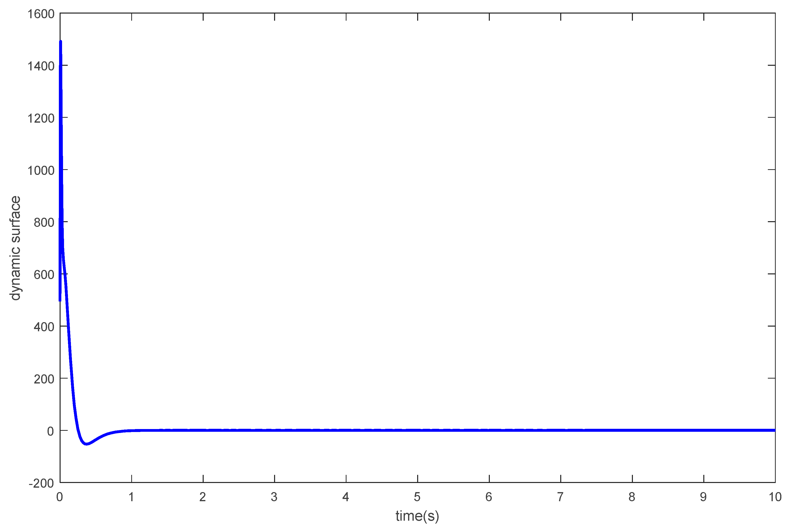
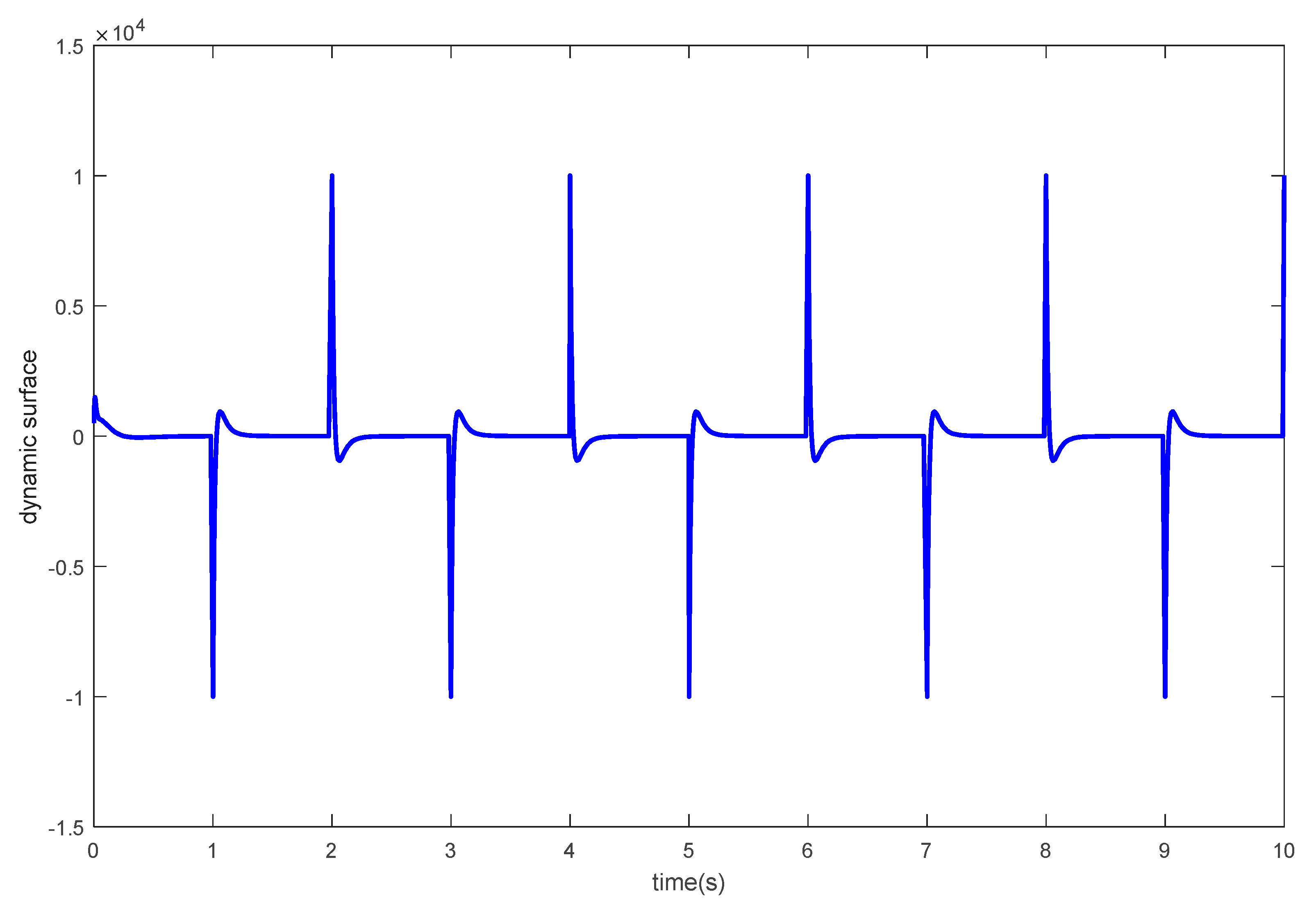
The time response of dynamic surface is shown in Figure 9. It can be seen that the response curve is smooth without chattering.

In order to further verify the control effect of the proposed method, we changed the desire glue flow to a square signal with an amplitude of 10 and the disturbance to noisy random signals; the initial values of the HGO and the first-order low-pass filters remained unchanged. The simulation results are shown in Figure 10, Figure 11, Figure 12, Figure 13 and Figure 14.

The simulation results showed that the proposed control method could still maintain good performance in spite of noise disturbance. When the glue flow input signal was constantly changing, the output of the system could still track the desire value quickly and accurately. For the immeasurable signals of the system, the HGO could estimate its value quickly and the track error was near 0, which meant the estimation could be controlled by replacing the actual value.

5. Conclusions

In this paper, the glue flow tracking control problem was investigated for particleboard glue mixing and dosing system in the presence of external disturbance caused by the pump, channel, and flow sensor. In the proposed compound controller, the system input signal’s derivative is estimated by HGO for feedback to the sliding-mode dynamic surface controller and to deal with various disturbances. Closed-loop system stability and tracking performance were testified and analyzed using a rigorous Lyapunov analysis. The efficiency of the proposed methods was verified by simulation, which showed that good performance was guaranteed.

References

1. Saravia-Cortez, A.M.; Herva, M.; García-Diéguez, C.; Roca, E. Assessing environmental sustainability of particleboard production process by ecological footprint. J. Clean. Prod. 2013, 52, 301–308. [Google Scholar] [CrossRef]
2. Wong, D.C.; Kozak, R.A. Particleboard performance requirements of secondary wood products manufacturers in Canada. For. Prod. J. 2008, 58, 34–41. [Google Scholar]
3. Padula, F.; Visioli, A. Tuning rules for optimal PID and fractional-order PID controllers. J. Process Control 2011, 21, 69–81. [Google Scholar] [CrossRef]
4. Lee, C.-H.; Chang, F.-K. Fractional-order PID controller optimization via improved electromagnetism-like algorithm. Expert Syst. Appl. 2010, 37, 8871–8878. [Google Scholar] [CrossRef]
5. Sharma, R.; Rana, K.P.S.; Kumar, V. Performance analysis of fractional order fuzzy PID controllers applied to a robotic manipulator. Expert Syst. Appl. 2014, 41, 4274–4289. [Google Scholar] [CrossRef]
6. Golestan, S.; Monfared, M.; Freijedo, F.D.; Guerrero, J.M. Performance improvement of a prefiltered synchronous-reference-frame PLL by using a PID-type loop filter. IEEE Trans. Ind. Electron. 2014, 61, 3469–3479. [Google Scholar] [CrossRef]
7. Xu, J.X.; Guo, Z.Q.; Tong, H.L. Design and Implementation of Integral Sliding-Mode Control on an Underactuated Two-Wheeled Mobile Robot. IEEE Trans. Ind. Electron. 2014, 61, 3671–3681. [Google Scholar] [CrossRef]
8. Sun, H.; Li, S.; Sun, C. Finite time integral sliding mode control of hypersonic vehicles. Nonlinear Dyn. 2013, 73, 229–244. [Google Scholar] [CrossRef]
9. Lee, J.Y. Variable PID Gain Tuning Method Using Backstepping Control With Time-Delay Estimation and Nonlinear Damping. IEEE Trans. Ind. Electron. 2014, 61, 6975–6985. [Google Scholar] [CrossRef]
10. Shen, Q.; Jiang, B.; Cocquempot, V. Adaptive fault-tolerant backstepping control against actuator gain faults and its applications to an aircraft longitudinal motion dynamics. Int. J. Robust Nonlinear Control 2013, 23, 1753–1779. [Google Scholar] [CrossRef]
11. Das, A.; Lewis, F.; Subbarao, K. Dynamic Neural Network-Based Robust Backstepping Control approach for Quadrotors. In Proceedings of the AIAA Guidance, Navigation and Control Conference and Exhibit, Honolulu, HI, USA, 18–21 August 2013. [Google Scholar]
12. Swaroop, D.; Gerdes, J.C.; Yip, P.P.; Hedrick, J.K. Dynamic surface control of nonlinear systems. In Proceedings of the American Control Conference, Albuquerque, NM, USA, 6 June 1997; Volume 5, pp. 3028–3034. [Google Scholar]
13. Xu, B.; Yang, C.; Pan, Y. Global neural dynamic surface tracking control of strict-feedback systems with application to hypersonic flight vehicle. IEEE Trans. Neural Netw. Learn. Syst. 2017, 26, 2563–2575. [Google Scholar] [CrossRef] [PubMed]
14. Wang, H.; Wang, D.; Peng, Z. Neural network based adaptive dynamic surface control for cooperative path following of marine surface vehicles via state and output feedback. Neurocomputing 2014, 133, 170–178. [Google Scholar] [CrossRef]
15. Qian, M.S.; Jiang, B.; Xu, D.Z.; Chen, F.Y. Robust dynamics surface fault tolerant control design for attitude control systems of UAV. Syst. Eng. Electron. 2014, 36, 1798–1803. [Google Scholar]
16. Cho, D.; Kang, S.; Kim, H.J. Adaptive dynamic surface control based on neural network for missile autopilot. In Proceedings of the AIAA Guidance, Navigation, and Control Conference, Honolulu, HI, USA, 18–21 August 2013. [Google Scholar]
17. Zhang, C.; Wu, Y.J. Non-singular terminal dynamic surface control based integrated guidance and control design and simulation. ISA Trans. 2016, 63, 112–120. [Google Scholar]
18. Precup, R.E.; Radac, M.B.; Roman, R.C.; Petriu, E.M. Model-free sliding mode control of nonlinear systems: Algorithms and experiments. Inf. Sci. 2017, 381, 176–192. [Google Scholar] [CrossRef]
19. Incremona, G.P.; Cucuzzella, M.; Ferrara, A. Adaptive suboptimal second-order sliding mode control for microgrids. Int. J. Control 2016, 89, 1–37. [Google Scholar] [CrossRef]
20. Komurcugil, H.; Biricik, S. Time-varying and constant switching frequency based sliding mode control methods for transformerless DVR employing half-bridge VSI. IEEE Trans. Ind. Electron. 2017, 64, 2570–2579. [Google Scholar] [CrossRef]
21. Bourouba, B.; Ladaci, S. Robust Fuzzy Adaptive Sliding Mode Stabilization for Fractional-Order Chaos. Algorithms 2018, 11, 101. [Google Scholar] [CrossRef]
22. Vrkalovic, S.; Lunca, E.C.; Borlea, I.-D. Model-free sliding mode and fuzzy controllers for reverse osmosis desalination plants. Int. J. Artif. Intell. 2018, 16, 208–222. [Google Scholar]
23. Tong, S.; Ren, C.E.; Li, Y. Adaptive Fuzzy Decentralized control for nonlinear large-scale systems based on high-gain observer. Chin. Control Decis. Conf. 2012, 55, 228–242. [Google Scholar] [CrossRef]
24. Ren, C.; Chen, C.L.P. Decentralized control for second-order uncertain nonlinear multi-agent systems consensus problem based on fuzzy adaptive high-gain observer. In Proceedings of the IEEE International Conference on Systems, Man, and Cybernetics, Manchester, UK, 13–16 October 2013; pp. 4935–4940. [Google Scholar]
25. Mercorelli, P. A two-stage sliding-mode high-gain observer to reduce uncertainties and disturbances effects for sensorless control in automotive applications. IEEE Trans. Ind. Electron. 2015, 62, 5929–5940. [Google Scholar] [CrossRef]
26. Guo, Q.; Jiang, D.; Yu, T. High-gain observer-based output feedback control of single-rod electro-hydraulic actuator. IET Control Theory Appl. 2015, 9, 2395–2404. [Google Scholar] [CrossRef]
27. Bou Serhal, R.E.; Khalil, H.K. Application of the extended high gain observer to underactuated mechanical systems. In Proceedings of the American Control Conference, Montreal, QC, Canada, 27–29 June 2012; pp. 4727–4732. [Google Scholar]
28. Veluvolu, K.C.; Defoort, M.; Soh, Y.C. High-gain observer with sliding mode for nonlinear state estimation and fault reconstruction. J. Frankl. Inst. 2014, 351, 1995–2014. [Google Scholar] [CrossRef]
29. Ayadi, A.; Hajji, S.; Smaoui, M.; Chaari, A.; Farza, M. A high gain observer coupled to a sliding mode technique for electropneumatic system control. In Proceedings of the International Conference on Sciences and Techniques of Automatic Control and Computer Engineering, Hammamet, Tunisia, 21–23 December 2015; pp. 963–967. [Google Scholar]
30. Choi, C.; Tsao, T.C.; Matsubara, A. Control of linear motor machine tool feed drives for end milling: Robust MIMO approach. In Proceedings of the American Control Conference, San Diego, CA, USA, 2–4 June 1999. [Google Scholar]
31. Hamidat, A.; Benyoucef, B. Mathematic models of photovoltaic motor-pump systems. Renew. Energy 2008, 33, 933–942. [Google Scholar] [CrossRef]
32. Ioannou, P.A.; Sun, J. Robust Adaptive Control; Prentice-Hall: Englewood Cliffs, NJ, USA, 1996. [Google Scholar]
Figure 1. Particleboard glue mixing and dosing system.
Algorithms 11 00166 g001
Figure 2. The basic structure of flow control system.
Algorithms 11 00166 g002
Figure 3. Configuration of the compound controller.
Algorithms 11 00166 g003
Figure 4. Flowchart of the proposed control algorithm.
Algorithms 11 00166 g004
Figure 5. Time response of glue flow tracking and tracking error.
Algorithms 11 00166 g005
Figure 6. Time response of the first-order low-pass filter. ×2p and ×3p represent the input of the first-order low-pass filter x ¯ 2 and x ¯ 3 , respectively; ×2d and ×3d represent the output of the first-order low-pass filter x 2 d and x 3 d , respectively.
Algorithms 11 00166 g006
Figure 7. Comparison of the actual and estimated values of the system input.
Algorithms 11 00166 g007
Figure 8. Comparison of the actual and estimated values of the system input.
Algorithms 11 00166 g008
Figure 9. Time response of dynamic surface.
Algorithms 11 00166 g009
Figure 10. Time response of glue flow tracking and tracking error.
Algorithms 11 00166 g010
Figure 11. Time response of the first-order low-pass filter. ×2p and ×3p represent the input of the first-order low-pass filter x ¯ 2 and x ¯ 3 , respectively; ×2d and ×3d represent the output of the first-order low-pass filter x 2 d and x 3 d , respectively.
Algorithms 11 00166 g011
Figure 12. Comparison of the actual and estimated values of the system input.
Algorithms 11 00166 g012
Figure 13. Comparison of the actual and estimated values of the system input.
Algorithms 11 00166 g013
Figure 14. Time response of dynamic surface.
Algorithms 11 00166 g014