1. Introduction
Learning techniques in soft computing exist for the purpose of adjusting models so they can accurately represent data in some domain. Although there are various approaches to these learning techniques, we can categorize learning techniques into two groups: hybrid and non-hybrid learning techniques.
A non-hybrid learning technique is composed of a single algorithmic process which achieves the learning of a model, whereas a hybrid learning technique is composed of a sequence of two or more algorithms where in each step a portion of the final model is achieved. Some examples of non-hybrid techniques are a learning algorithm for multiplicative neuron model artificial neural networks [
1], an optimized second-order stochastic learning algorithm for neural network training using bounded stochastic diagonal Levenberg–Marquardt [
2], design of interval type-2 fuzzy logic systems by utilizing the theory of an extreme learning machine [
3], the well-known backpropagation technique for artificial neural networks [
4], etc. Yet by combining some of these direct approaches with each other or with other techniques, their performance can greatly improve, such that some steps can compensate performance loss or simply focus on optimizing a portion of the model. Examples of such hybrid models are the scoring criterion for hybrid learning of two-component Bayesian multinets [
5], hybrid learning particle swarm optimization with genetic disturbance intended to combat the problem of premature convergence observed in many particle swarm optimization variants [
6], a hybrid Monte Carlo algorithm used to train Bayesian neural networks [
7], a learning method for constructing compact fuzzy models [
8], etc.
When dealing with raw data where models must be created, transforming such data into more manageable and meaningful information granules can greatly improve how the model performs as well as reducing the computational load of the model. An information granule is a representation of some similar information which can be used to model a portion of some domain knowledge. By forming multiple information granules, these can represent the totality of the information from which data is available; therefore, forming a granular model. Granular computing [
9,
10] is the paradigm to which these concepts belong.
Information granules which intrinsically support uncertainty can be represented by general type-2 fuzzy sets (GT2 FSs), and in turn these GT2 FSs can be inferred by a general type-2 fuzzy logic system (GT2 FLS) [
11]. Although, when dealing with type-2 fuzzy logic systems, they are either in the form of interval type-2 FSs [
12] or general type-2 FSs, interval type-2 FSs being a simplification of general type-2 FSs. In simple terms, uncertainty in a GT2 FS is represented by a 3D volume, while uncertainty in an IT2 FS is represented by a 2D area. It is not until recent years that research interest has gained momentum for GT2 FLSs; examples of such published research are fuzzy clustering based on a simulated annealing meta-heuristic algorithm [
13], similarity measures
α-plane representation [
14], hierarchical collapsing method for direct defuzzification [
15], a multi-central fuzzy clustering approach for pattern recognitions [
16], etc.
Apart from Mamdani FLSs which represent consequents with membership functions, there also exists the representation by linear functions. These FLSs are named Takagi–Sugeno–Kang fuzzy logic systems (TSK FLSs). Examples of TSK FLS usage are evolving crane systems [
17], fuzzy dynamic output feedback control [
18], analysis of the dengue risk [
19], predicting the complex changes of offshore beach topographies under high waves [
20], clustering [
21], etc.
As published research with GT2 FLS is still very limited, most of it uses Mamdani FLSs, and so far only two published journal papers using a GT2 TSK FLS exist, for controlling a mobile robot [
22], and data-driven modeling via a type-2 TSK neural network [
23].
In this paper, a proposal of a hybrid learning technique for GT2 TSK FLSs is given, which (1) makes use of the principle of justifiable granularity in order to define a degree of uncertainty in information granules; and (2) a double least square error learning technique is used in order to calculate the parameters for IT2 TSK linear functions. In addition, it is fair to say that at the time of writing of this paper, published research of GT2 TSK FLSs is very limited, therefore this paper contributes to the possibilities that can be achieved by representing consequents with TSK linear functions instead of the more common Mamdani consequents for GT2 FLSs.
This paper is separated into four main sections. First, some background is given which introduces the basic concepts used in the proposed hybrid learning technique; then, the proposed hybrid learning technique is thoroughly described; afterwards, some experimental data is given which defines the general performance of the technique; finally, some concluding remarks are given.
2. Background
2.1. General Type-2 Fuzzy Logic Systems with Interval Type-2 TSK Consequents
A general type-2 fuzzy set (GT2 FS) defined by
is represented by
, where
is the Universe of Discourse and
. In
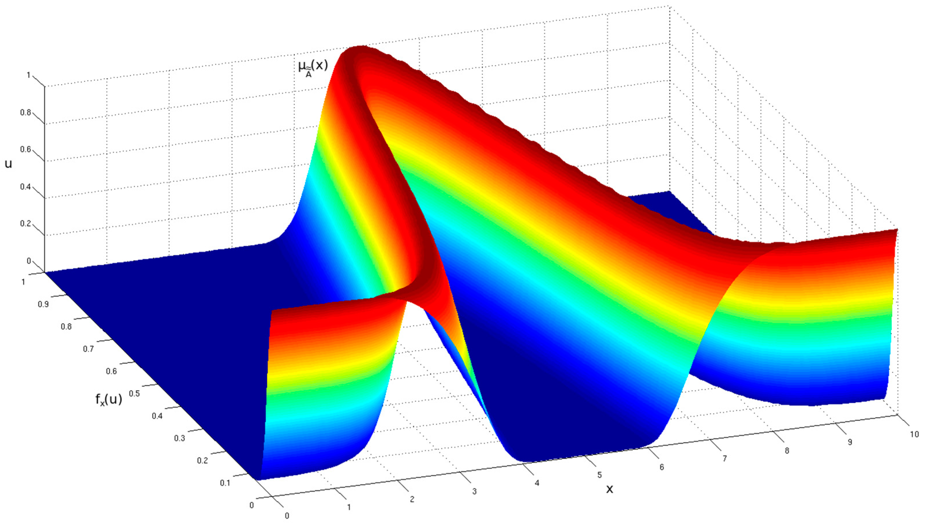
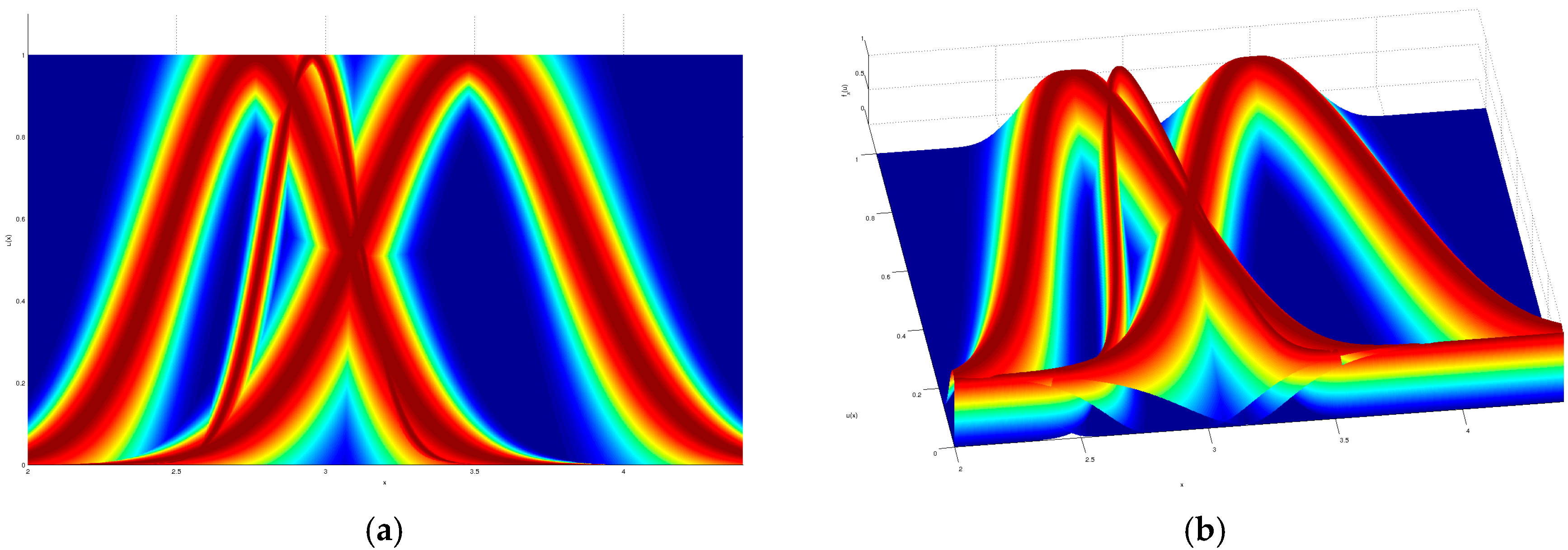
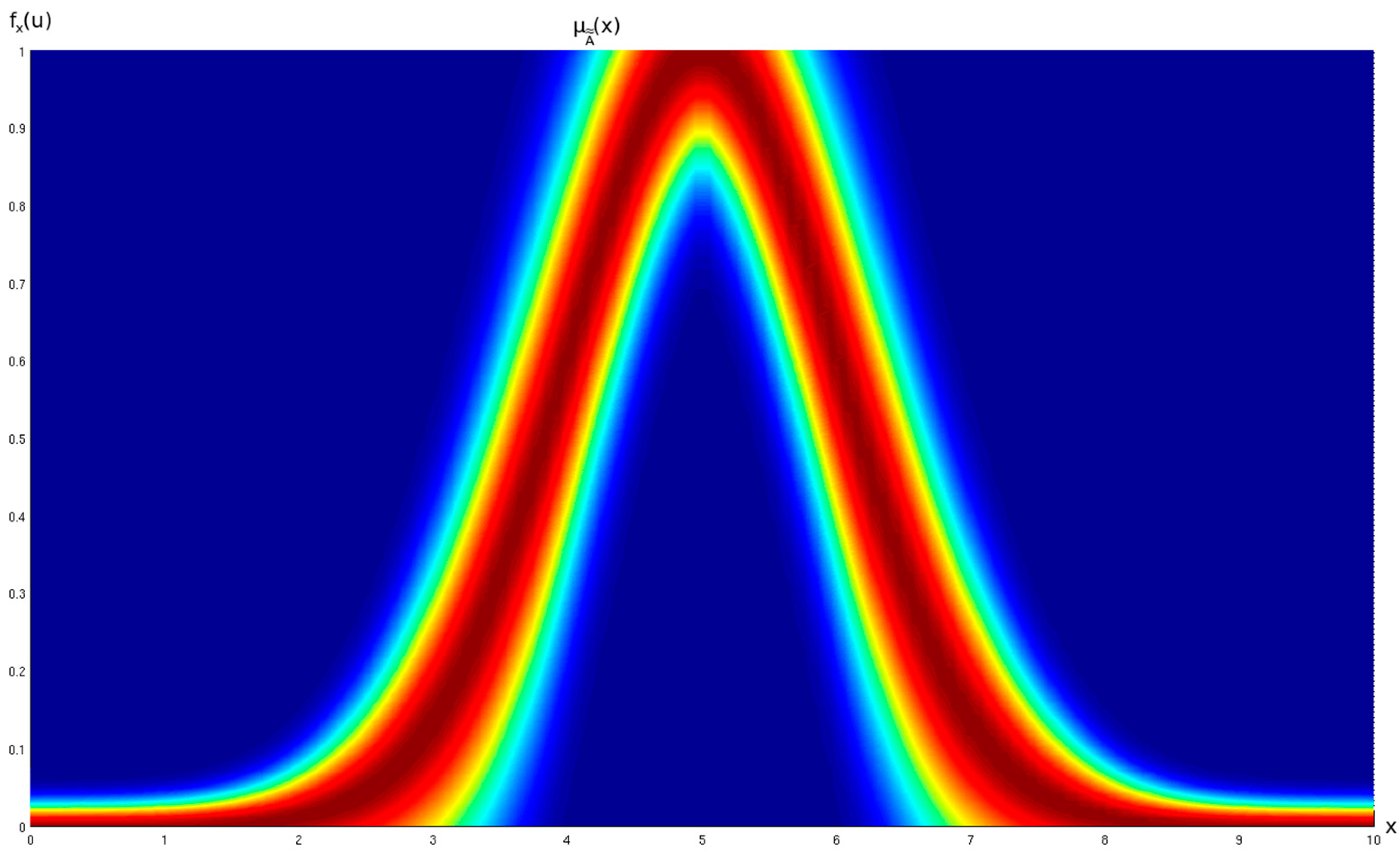
Figure 1, a generic GT2 FS is shown from the primary membership function’s perspective. In
Figure 2, the same generic GT2 FS is shown but from an isometric view.
The rules of a GT2 FLS are in the form of Equation (1), where
is the
q-th rule,
is the
p-th input,
is a membership function on the
q-th rule and
p-th input,
is an interval type-2 Takagi–Sugeno–Kang (IT2 TSK) linear function on the
q-th rule.
An IT2 TSK linear function [
24]
takes the form of Equations (2) and (3), where
and
are the left and right switch points of the IT2 TSK linear function on the
q-th rule,
is the
k-th coefficient on the
q-th rule,
is the
k-th input,
is the constant on the
q-th rule,
is the spread
k-th coefficient on the
q-th rule, and
is the spread on the constant on the
q-th rule.
2.2. General Type-2 Membership Function Parameterization
The proposed hybrid learning technique depends on the parameterization of a GT2 FS in the form of a Gaussian primary membership function with uncertain mean and Gaussian secondary membership functions. This GT2 membership function requires four parameters:
is the standard deviation of the primary membership function,
and
are the left and right centers of the Gaussian membership function with uncertain mean, and
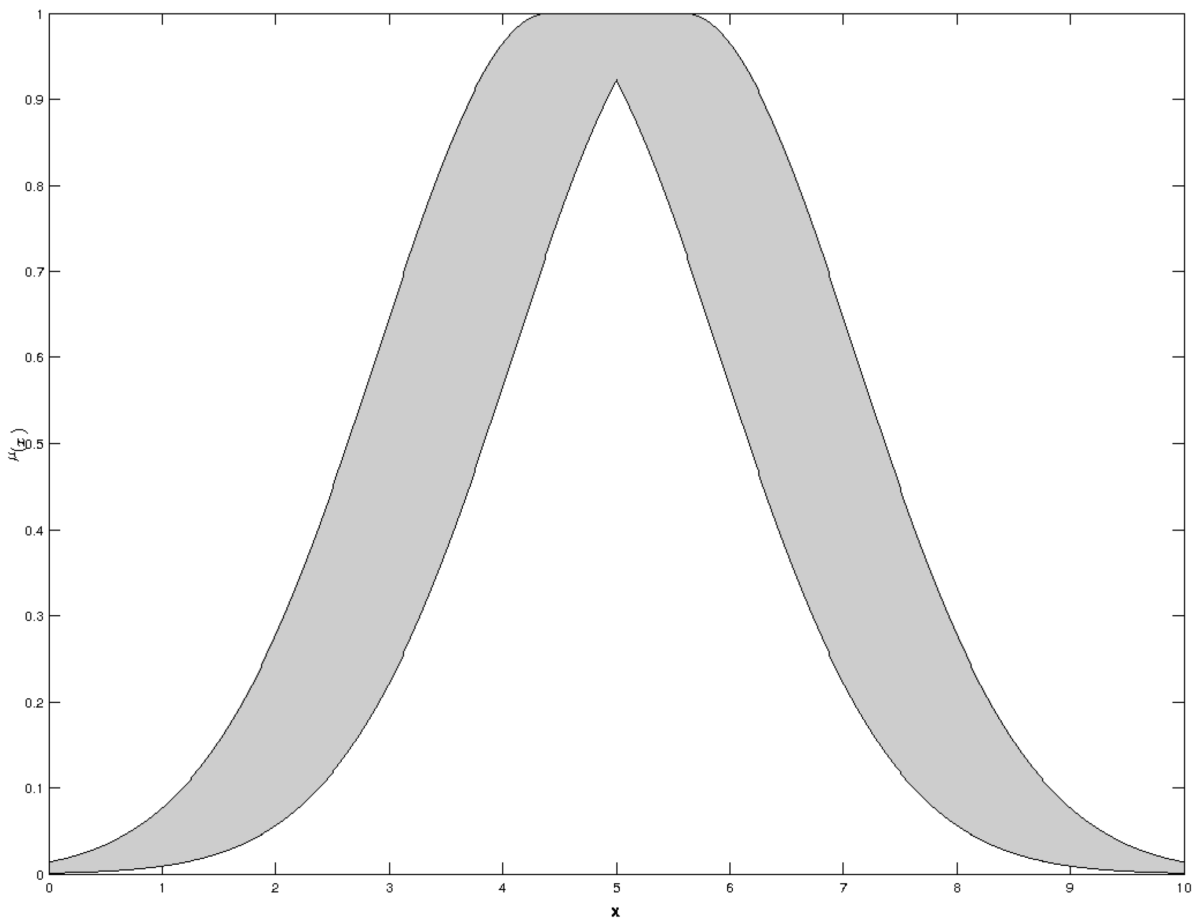
is a fraction of uncertainty which affects the support of the secondary membership function. Here, for the sake of simplification, the primary membership function is best represented by the support footprint of uncertainty (FOU) of the primary membership function in the form of an IT2 membership function, as shown in
Figure 3. Based on the parameterized structure of the support FOU, the hybrid learning technique performs two type-1 TSK optimizations, as if optimizing two distinct type-1 TSK FLSs.
The parameterization of the GT2 membership function is as follows. First, the support of the GT2 membership function is created by Equations (4)–(7), using
, where
on the Universe of Discourse
, and
such that
. Creating an IT2 MF with
and
, for the upper and lower membership function respectively, as shown in
Figure 3.
Afterwards, all parameters required to form the individual secondary membership functions must be calculated, as shown in Equations (8)–(10), where
and
are the center and standard deviation of the secondary Gaussian membership function, and
is a very small number, e.g., 0.000001.
Finally, each secondary membership function can be calculated by Equation (11), such that
is the secondary function on
. Therefore, forming a complete GT2 membership function would be achieved by calculating for all
.
2.3. Principle of Justifiable Granularity
The purpose of this principle [
25] is to specify the optimal size of an information granule where sufficient coverage for experimental data exists while simultaneously limiting the coverage size in order to not overgeneralize. These differences are shown in
Figure 4.
A dual optimization must exist which can consider both objectives, where (1) the information granule must be as specific as possible; and (2) the information granule must have sufficient numerical evidence.
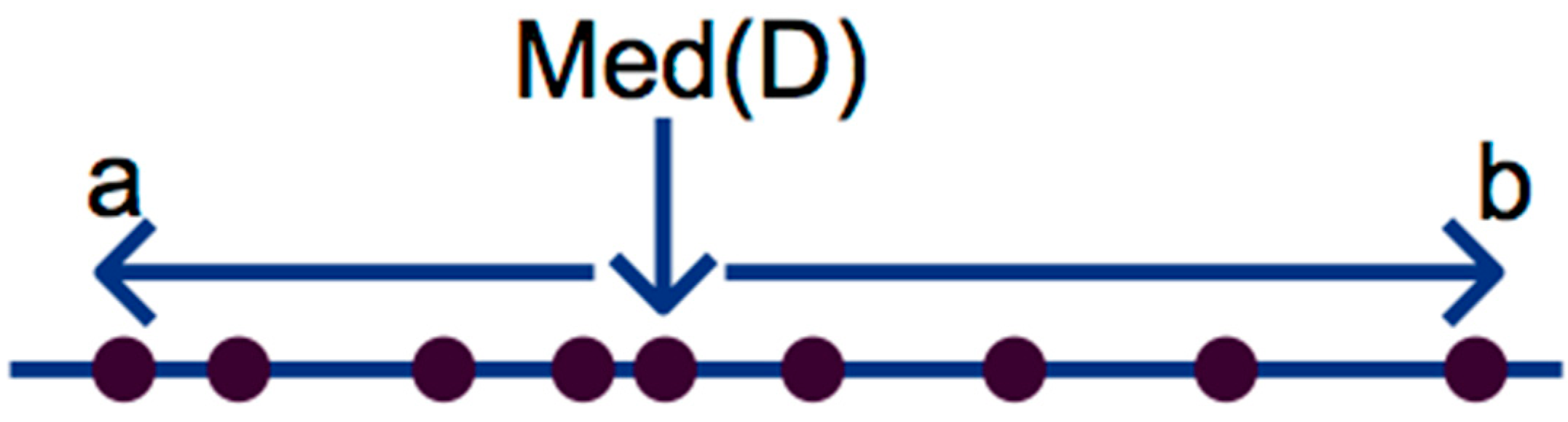
As the length of an information granule is perceived by two delimiting sides of an interval, the dual optimization is performed once per each side. As shown in
Figure 5, the left side interval from the Median of the data sample
a and the right side interval from the Median of the data sample
b creates two intervals to be optimized, where
Med(
D) is the Median of available data
D which initially constructed said information granule.
Shown in Equations (12) and (13) are the search equations
V() for optimizing
a and
b respectively, where
V() is an integration of the probability density function from
Med(
D) to all prototypes of
a, or
b, multiplied by the user criterion for specificity
α, where
α is a variable which affects the final length of
a or
b, such that
has the highest experimental data, and
represents the most specific possible length and has minimal experimental data.
3. Description of the Hybrid Learning Technique for GT2 TSK FLS
The proposed approach, being hybrid in nature, is composed of a sequence of multiple steps, each using different algorithms in order to achieve the final model which is shown in this section.
The hybrid learning technique requires a set of meaningful centers
for the antecedents of the rule base, these can be obtained via any method, such as clustering algorithms; for this paper, a fuzzy c-means (FCM) clustering algorithm [
26] was used. Via these cluster centers, subsets belonging to each cluster center are selected through Euclidean distance, where the nearest data point to each cluster center is a member of its subset.
After all subsets are found, cluster coverages can be calculated, i.e., the standard deviation σ, obtained through Equation (14), where
is the standard deviation of the
q-th rule and
k-th input,
is each datum from the subsets previously obtained,
is the cluster center for the
q-th rule and
k-th input, and
n is the cardinality of the subset.
Up to now, a Type-1 Gaussian membership function can be formed with . However, the sought end product is a GT2 Gaussian primary membership function with uncertain mean and Gaussian secondary membership functions, which requires the parameters: . So far, we have calculated and partially and , which are based on . The following process obtains the remaining required parameters to form GT2 FSs of the antecedents.
To obtain
and
, the principle of justifiable granularity is used as a means to heuristically measure uncertainty via the difference of the intervals
a and
b. This is carried out by extending each information granule to its highest coverage by using the user criterion value of
for each side of the information granule’s interval, as described by Equations (12) and (13). When both intervals
a and
b are obtained, their difference will define the amount of uncertainty which will be used to calculate parameters
, as shown in Equation (15), where
τ is a measure of uncertainty for the
q-th rule and
k-th input.
The obtained value of
τq,k is used by Equations (16) and (17) to offset the centers
of the Gaussian primary membership function by adding uncertainty in the mean, thus obtaining
.
For practical reasons, the final missing value of
is set to zero
for all membership functions, as it was found that it has no effect on classification performance if other values are set; some experimentation to demonstrate this is shown in
Section 4. This ends the parameter acquisition phase for all antecedents in the GT2 TSK FLS.
All IT2 linear TSK consequents are calculated in a two-step process. First, a Least Square Estimator (LSE) algorithm [
27,
28] is used twice; as the Gaussian primary membership function with uncertain mean is parameterized by a left and right T1 Gaussian membership function on the support FOU, the LSE is applied as if two T1 TSK FLSs existed, using the following sets of parameters: for the left
and right side
. When all TSK coefficients
are obtained, the average of both sets of parameters is used, as shown in Equation (18), where
and
are the coefficient sets for the left and right side respectively. This set
C represents all
cq,k coefficients of all IT2 TSK linear equations.
The second and final part of the process for calculating the final spreads
of each coefficient, in set
S, which is carried out by measuring the absolute difference between each coefficient set,
and
, as shown in Equation (19).
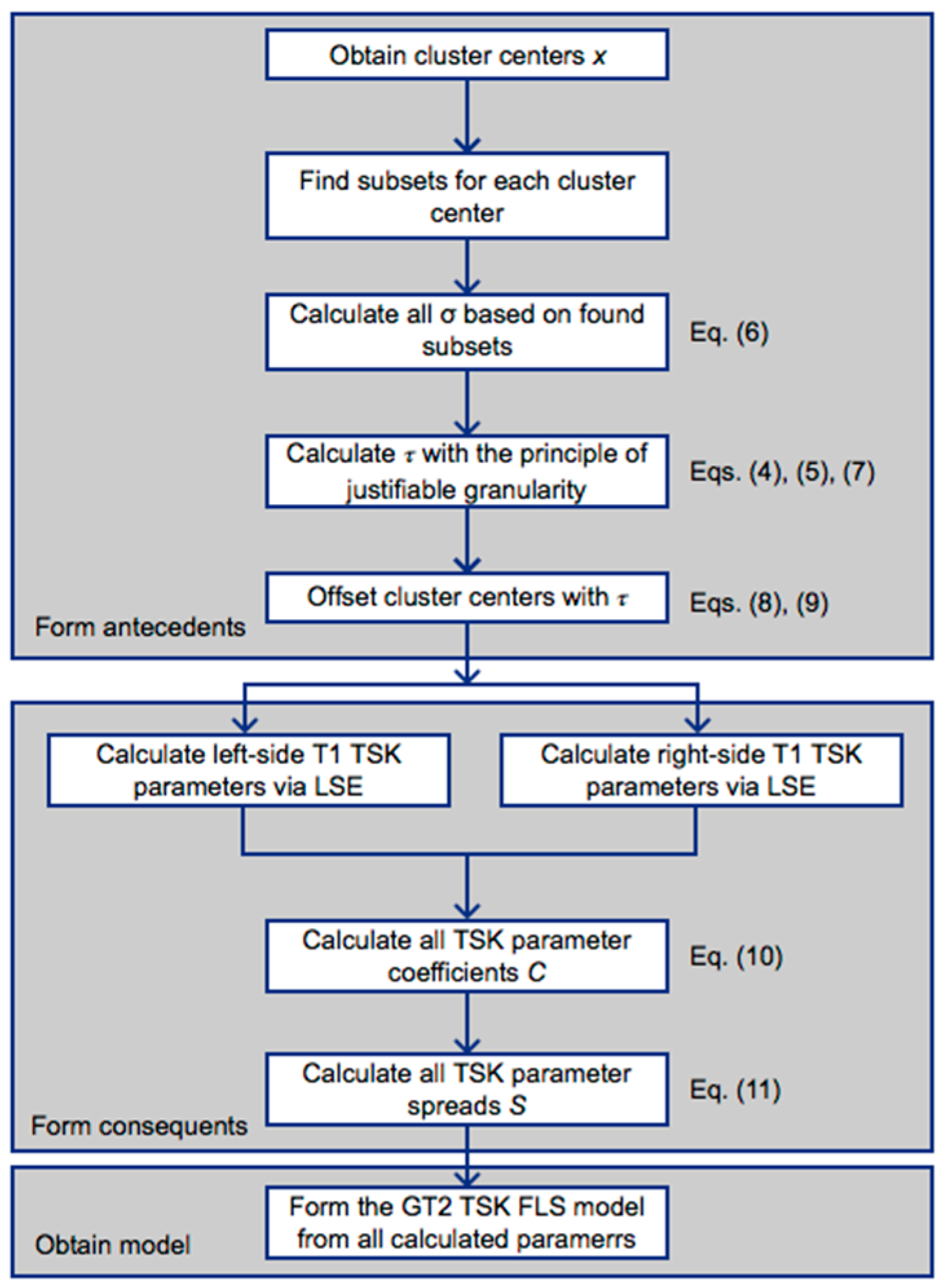
A schematic of the proposed hybrid algorithm is shown in
Figure 6, where all steps described in this section concentrate the sequence to obtain the antecedents and consequents of the GT2 TSK FLS model, as well as associating certain key steps to their corresponding equations.
4. Experimentation and Results Discussion
A set of various experiments was conducted with classification benchmark datasets in order to explore the effectiveness of the proposed hybrid algorithm.
Table 1 shows a compact description of used classification benchmarks [
29].
Experimentation was done using Hold-Out data separation, with 60% randomly selected training data and 40% test data, showing the mean value and standard deviation of 30 execution runs. Concerning the number of rules used per each class, in principle, better model generalization is usually achieved by reducing the number of rules per class, instead of increasing the number of rules and possibly falling into a case of overfitting [
30,
31,
32]. For that reason and for simplification purposes, one-rule-per-class was used for all experiments, i.e., results for the iris dataset, which has three classes, were represented by three fuzzy rules, and so on.
Results are shown in
Table 2, where values in bold achieved the best performance. Results were compared to Fuzzy C-Means (FCM) [
26], Subtractive algorithm [
33], Decision Trees, Support Vector Machine (SVM) [
34], K-Nearest Neighbors (KNN) [
35], and Naïve Bayes [
36]; and it must be noted that since the common SVM is designed only for binary classification, it cannot work with datasets which have three or more classes, marked with (-). Performance is measured through total classification percentage, where very good and stable results, in general, are achieved by the proposed hybrid learning technique. Values inside ( ), next to each classification percentage, are the standard deviations for the 30 executions runs which achieved each result, where lower values are better and higher are worse; it can be seen that the proposed hybrid algorithm has a general low variance in the obtained results by means of the calculated standard deviation, yet in the wine dataset it had much more variance when compared to the rest of the techniques.
Although the proposed hybrid technique does not always achieve the best results, it does achieve a better overall performance, as shown in
Table 3, where the average across the overall dataset results is shown, such that a higher value means better performance in general, demonstrating that the proposed technique is more stable in general.
In
Table 4, an experiment to demonstrate that the value of
has no effect whatsoever in the classification performance of the proposed hybrid learning technique is shown. Two datasets were chosen at random with 60% training data and 40% testing data, with
. To achieve a truer experiment when comparing chosen
values, the exact same training data and testing data was used, i.e., with each execution run, data was not randomly separated into a 60/40 partition; instead, the partition was fixed with exact data in each experiment, and only the value of
was changed.
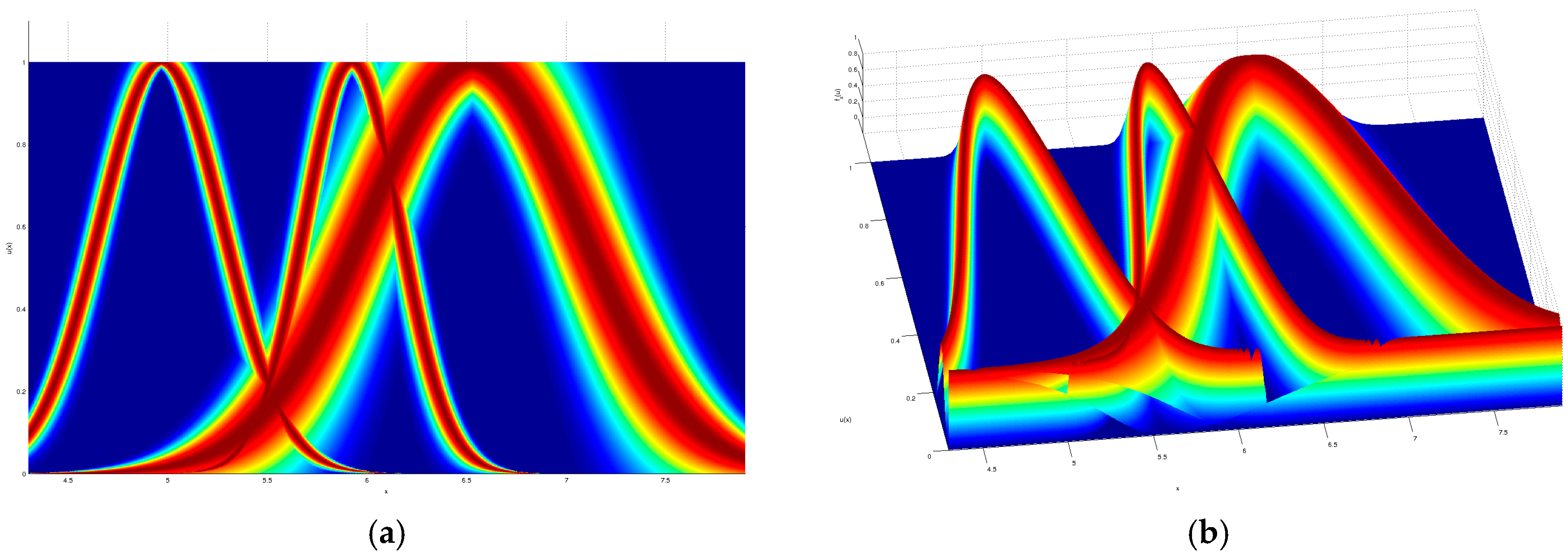
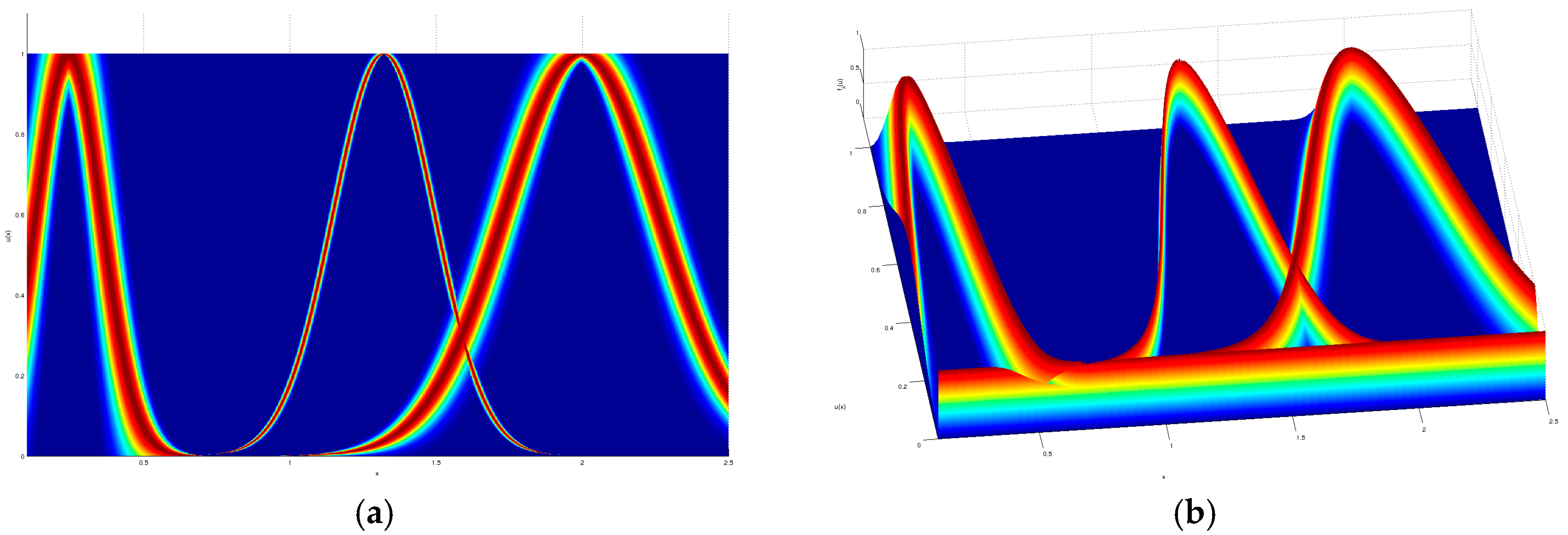
As a visual example, the input partition for the iris dataset modeled by a GT2 TSK FLS which obtained the given result in
Table 2, is shown in
Figure 7,
Figure 8,
Figure 9 and
Figure 10, where a top and orthogonal view can be seen; in all accounts, the amount of uncertainty within each membership function is quite contrasting, as there are membership functions with barely any uncertainty and also membership functions with quite a lot of uncertainty.
It must also be noted that there are a couple of variables where classification performance could be improved. First, as the initial hybrid learning technique requires prototype centers to begin constructing the GT2 FSs around them, if better prototypes are found, then the classification performance is also bound to improve; for the included experimentation in this paper, a FCM clustering algorithm was used to obtain the initial prototypes, yet other techniques could be used to improve the final classification performance by providing better quality initial prototypes. As is known, different techniques perform differently with each dataset, therefore by changing this part of the proposed hybrid algorithm, better results could be expected. Second, in this paper, GT2 FSs in the form of Gaussian primary membership functions with uncertain mean and Gaussian secondary membership functions were used, meaning that other GT2 FSs could be used; this, in itself, is worth exploring in future research, as different FSs could greatly improve the representation of information granules and therefore improve the quality of the fuzzy model. Third, a dual LSE application technique was used to calculate IT2 TSK linear function parameters for all consequents, where other more robust algorithms could be used to further improve the general performance of the model, e.g., Recursive Least Squares (RLS) algorithm.
One of the qualities of the proposed hybrid approach, as shown through experimentation, is the stability inherent in FLSs in general, especially in GT2 FLSs, where the integrated handling of uncertainty in its model permits less variance in achieved performance when compared to other classifying techniques. By using information granules which support varying degrees of uncertainty, as acquired by the same data which formed it, changing patterns in data have less of an effect on the performance of the fuzzy model created by the proposed hybrid technique.
5. Conclusions
The work proposed in this paper is an initial exploration into the effectiveness of GT2 TSK FLSs for use in classification scenarios. Due to the complexity of GT2 FLSs in general, a hybrid learning technique is introduced. As a result of using a hybrid learning algorithm, a sequence of various stages takes place in order to obtain the final fuzzy granular model; in the first stage, initial prototypes must be acquired from a sample of data; this can be obtained through various means, such as clustering algorithms, providing the flexibility of using any technique which may acquire these initial prototypes with improved quality; in the second stage, some level of uncertainty is defined through the principle of justifiable granularity, where differences between both intervals, a and b, for each information granule, depict how the spread of data measures uncertainty. The highest coverage is used in both intervals to simplify the information granule’s coverage, yet it could be possible to achieve better performance by identifying an optimal value between rather than just using equally for all information granules. Finally, the calculation stage of the IT2 TSK linear function parameters is a direct method reliant on the previous stage which obtains results via a dual application of the LSE algorithm, after which these two sets of parameters are joined to the final required parameters to finish forming the GT2 TSK FLS, where other more precise learning techniques should yield much better parameters for improved model quality.
Experimentation gave a quick view of the general quality of these GT2 TSK FLS models, where a degree of stability was achieved in contrast to other more common classification algorithms. Research into GT2 TSK FLS is still scarce, and this paper showed some of the benefits of model quality, performance, and stability, that this type of system can achieve.


