Abstract
In this paper, we extend the analysis of the Lagged Diffusivity Method for nonlinear, non-steady reaction-convection-diffusion equations. In particular, we describe how the method can be used to solve the systems arising from different discretization schemes, recalling some results on the convergence of the method itself. Moreover, we also analyze the behavior of the method in case of problems presenting boundary layers or blow-up solutions.
1. Introduction
Let us consider the nonlinear, non-steady reaction-convection-diffusion equation
where is the initial time, is the density function, is the diffusion coefficient, is the velocity vector (assumed constant), is the absorption term, is the rate of change of the reaction and is the source term. This equation is important in various different fields and it can describe several processes and applications.
If we discretize Equation (1), at each time level the differential problem can be approximated by a nonlinear, algebraic system. However, computing the solution of the discretized system is generally complicated. For instance, if we use a Newton’s method, we incur in the problem of computing the Jacobian matrix, which is usually difficult and computationally onerous. Therefore, it is suitable to first linearize the discretized system by setting up an iterative procedure which “lags” the diffusivity. In this way, we obtain the so-called Lagged Diffusivity Method (LDM). The analysis of this kind of strategies can be traced back to [1]. More recently, the LDM applied to steady and non-steady diffusion equations with reaction and/or convection terms has been studied in [2] and following works.
The nonlinear algebraic system is thus replaced by a series of systems of weakly nonlinear algebraic equations, whose Jacobian matrix is much easier to compute. Therefore, these systems can be easily solved by a Newton’s method. Lastly, at each Newton iteration we solve a system of linear algebraic equations (which we again do iteratively, for enhanced efficiency).
This paper addresses some topics which have not been considered in earlier works. In particular, we
- compare different discretizations. In particular, we consider what happens when the space is discretized by an upwind method or by central finite differences. We also describe different time discretizations, considering the -method and the IMEX schemes;
- study numerically what happens in some particularly critical cases, where some smoothness assumptions are not satisfied. This is the case of boundary layer and blow-up solutions.
Regarding the discretization, this is relevant since the discretization can modify the properties of the discretized systems. This can be exploited to improve the solution procedure: for instance, we notice that the upwind method can significantly reduce the computational times when is large (at the cost of a worse order of approximation).
The analysis of blow-up solutions is instead interesting for two reasons. First, we evaluate the behavior of the method in critical situations where the LDM is not analytically proven to converge. Indeed, the convergence of the method requires some smoothness assumptions on , , g and s which are not satisfied in proximity of blow-ups and boundary layers. Second, we analyze numerically the problem, while several papers regarding blow-up solutions deal with the analytical problem of determining if and when the blow-up occurs (e.g., if T is finite or not) and they are often referred to 1D differential problems with Neumann boundary conditions. Regarding analyses involving multidimensional domains and/or Dirichlet boundary conditions, it is instead worth citing [3,4,5], which are concerned with problems similar to the ones we analyze in the following. In particular, criteria for determining whether the blow-up occurs in a finite time or not and for estimating the blow-up time itself are given by using the Hopf’s maximum principle (e.g., see [6] (§2.3) or [7]). Other interesting papers on blow-up include [8,9], while [10] is a comprehensive review on blow-up in parabolic equations.
In Section 2 we analyze the discretization. In particular, we describe how the discretized system changes when space is discretized by central finite differences or by an up-wind scheme and when time is integrated by a method or by IMEX strategies.
In Section 3 we then summarize the method and consider how it is affected by the discretization itself. We also report some known results on the monotonicity of the finite-difference (FD) operators and on the convergence of the method.
In Section 4 we provide some details on the implementation, an algorithm and a short summary of the solution method.
Lastly, Section 5 is devoted to the numerical experiments. First, we show numerically the differences which arise when the discretization is changed. Then, we study problems characterized by blow-up and by boundary layer solutions in order to analyze the behavior of the LDM in critical cases, when the smoothness assumptions are not satisfied.
2. Discretization
2.1. Space Discretization
For simplicity, let us assume to be a 2D bounded rectangular domain. Let us superimpose a grid to . For simplicity, we use uniform mesh size h along x and y. Thus, is made of the mesh points , , with:
Using this grid, denotes the grid function which approximates the solution at the mesh points of , , . This grid function satisfies the initial condition for and and the Dirichlet boundary conditions for , .
We can now approximate the derivatives of Equation (1) by finite difference methods. In this regard, several choices are possible. In particular, it is interesting to analyze the space discretizations obtained by central finite differences and by the upwind scheme. Indeed, this choice influences the properties of the matrix of the discretized system, as we will see in the following. Regarding the upwind scheme, we consider, for instance, the case of positive . If < 0 the backward difference quotients which approximate the first-order derivatives are simply replaced by forward difference quotients.
Thus, denoting the forward finite differences (in x and in y respectively) by and , the backward finite differences by , and the central finite differences by , , we have:
- Discretization by central finite differences (error )
- Discretization by upwind scheme (error ), case > 0
In both cases, we can write the discretization in a more convenient way by defining
Then, setting (analogously for , , and ), the right hand-side of Equations (2) and (3) can be written formally in the same way as
In the following, we denote by for compactness of notation.
Finally, we use matrix notation to write the entire system of ordinary differential equations arising from the space discretization. In this regard, we use the row lexicographic ordering for mesh points and define with , for , . We can then write the vector containing all the at internal mesh points. Thus, the space discretization leads to
Again, we notice that formally this expression is valid both when the discretization is performed by central FD and when the upwind scheme is used. The following differences are however present:
- when we use the upwind scheme, the order of the approximation is ; when we use central FD, the order of the approximation is ;
- when we use the upwind scheme, is irreducibly diagonally dominant [11] (p. 23) irrespective of the choice of h. Having also positive diagonal elements and non positive off-diagonal elements, it is always a non-singular M-matrix [11] (p. 91). With central FD, is irreducibly diagonally dominant (and a non-singular M-matrix) only if h satisfies a condition on the step-size. In particular, by Equation (4) if is easy to find that this condition corresponds to
The vector in Equation (6) derives from the Dirichlet boundary conditions at points . Considering the Dirichlet BCs in Equation (1) and using, again, the row-lexicographic order, its components are
where the coefficients L, B, R, T depend on at the inner point which is neighbor to the considered point of . At corners, where the same inner point is neighbor to two boundary points, we then have two contributions: e.g., .
Defining , is the nonlinear mapping of components , with , and . It is, then, easy to notice that is a diagonal mapping [12] (p. 11).
Finally, contains the terms arising from the source term: with , and .
2.2. Time Discretization
We now consider time discretization. Let us introduce a time spacing , which defines a series of time levels: the n-th time level is defined by ,
The time derivatives of Equation (6) can be approximated by several different schemes. We could use, for example, the well-known method (e.g., see [13]), which is completely implicit when . An alternative, as noted in the Introduction, is given by IMEX methods, which have been employed to solve diffusion equations when convection or reaction terms can be treated explicitly.
For instance, let us apply the -method. Denoting by the approximation of (with solution of Equation (6) at ) and by , we get:
for and with .
By simple algebraic manipulations, we find that at each time level the vector is given by the solution of the nonlinear algebraic system
where , I is the identity matrix and is a vector containing the known terms, defined as
If we use an IMEX method, we similarly get a nonlinear algebraic system to solve at each time level. The difference is that some terms are treated explicitly. Thus, if, for instance, the reaction term is treated explicitly, at the time level the mapping is evaluated at time n; then becomes a known term which appears solely in the known vector .
Analogously, if the velocity is not linear, it could be useful to treat explicitly the convection term. In this case, the part of depending on would appear solely in the known vector .
3. The Lagged Diffusivity Method
We now introduce the lagged diffusivity method to solve the discretized system, referring, for instance, to Equation (9).
Solving Equation (9) by a Newton’s method would be onerous, since the Jacobian matrix of is generally hard to compute. The lagged diffusivity method, on the other hand, linearizes the discretized system by iteratively “lagging” the diffusivity term. At each iteration we must thus solve a weakly nonlinear algebraic system, whose Jacobian matrix is significantly easier to compute.
Let us study more in detail the procedure applied to Equation (9). Lagging the diffusivity means that the new iterate of the -th lagging iteration is the solution of the weakly nonlinear system
When is a nonsingular M-matrix, is evidently nonsingular .
Thus, we now have to solve Equation (10) at each lagging iteration. We can do this by a Newton’s method (or, in general, by an iterative method) which is stopped when the residual
satisfies a stopping criterion
where denotes the Euclidean norm and is a given tolerance such that for . When the inner solver converges, we find , which is used, in turn, to lag the diffusivity at the -th lagged iteration. Proceeding in the same way, we thus find and so on for the following iterations.
3.1. Effect of the Discretization
In the previous paragraphs, we applied the lagged diffusivity method to Equation (9), which was obtained by discretizing time using a method. The time discretization, however, affects some properties of the lagging iteration. For instance, if we can use an IMEX method and treat explicitly, the lagged diffusivity method completely linearizes the discretized system.
Analogously, an IMEX scheme can simplify the analysis of cases with non-constant velocity terms: if we can treat non-constant terms explicitly, all the convection terms are evaluated at the previous time level and are, thus, known. Both monotonicity and convergence analyses can then be traced back to the results obtained for constant .
Figure 1 summarizes all these cases, representing which functions are unknown at each time level and at each lagging iteration.
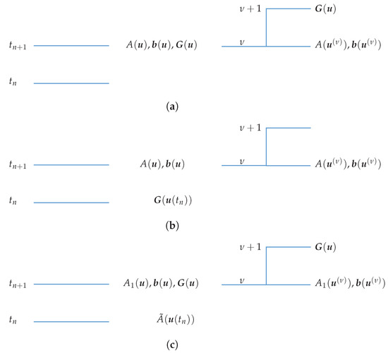
Figure 1.
Summary of the nonlinear terms present at each time level and at each lagging iteration for different time discretizations. (a) method; (b) IMEX scheme with explicit treatment of ; (c) IMEX scheme with non-constant velocity term treated explicitly. Here represents the part of A dependent on and represents the part of A dependent on .
Finally, although formally the system does not change, also the space discretization has an effect on the solution procedure. Indeed, we noticed earlier that is always an M-matrix when the upwind discretization is used, while we have a condition on the step-size h when central finite differences are used. If is an M-matrix, also the coefficient matrices of the linear systems arising from applying a Newton’s method to solve Equation (10) are M-matrices. This is important since some linear solvers converge only when the coefficient matrix is an M-matrix. We can thus always use these solvers when we use the upwind discretization, while we can do so only when condition Equation (7) is satisfied when we use central FD. This is of great importance especially when is large: indeed, in this case the coefficient matrix of the linear systems is highly non-symmetric and we would like to use splitting methods such as the Arithmetic Mean (AM) [14], which are particularly efficient in this case but require that the coefficient matrix is an M-matrix. Thus, also considering that Equation (7) implies that h must be really small when is large, we may want to use an upwind discretization in order to use these linear solvers. This is further studied in the numerical experiments.
3.2. Monotonicity of the Finite-Difference Operator and Convergence Analysis
Let us assume that the following smoothness properties hold true:
- the functions and g are continuous in u and continuously differentiable in . Moreover, the functions and s are continuous in their variables;
- is uniformly bounded in and : there exist two positive constants and such that . Moreover, we also assume and that is constant;
- for fixed , the function is Lipschitz continuous in u (uniformly in ) with constant ;
- for fixed , the function g is uniformly monotone in u (uniformly in ) with constant [15] (p. 114); moreover, it is continuously differentiable in u.
Under these smoothness assumptions, the monotonicity of the finite different operator and the convergence of the algorithm are assured for grid functions belonging to a set , where is a bound on the discrete norm and is a bound over the absolute value of the backward difference quotients of .
Thus, considering for instance the discretization by central finite differences and time integration by the method, the following theorems hold true
Theorem 1.
Let be a solution of the nonlinear system . If
then is uniformly monotone in and the solution of Equation (9) is unique.
Theorem 2.
The proofs of these theorems and more information on can be found in [16]. In the literature it is also possible to find proofs of the convergence of the procedure for less general cases (e.g., see [2] for steady state reaction diffusion problems). Proceeding analogously, similar results can be easily found also for the other discretizations.
4. Solution Procedure
In this section, we present some insights on the implementation that is used in the numerical experiments. This implementation follows the description in [2], with the difference that the inner systems are here solved by an inexact, simplified Newton iteration and that we use the correction on the initialization of tolerances presented in [16] and here summarized in Section 4.2. Then, we also briefly summarize the systems arising from the discretization and from the LDM and provide an algorithm which describes the entire procedure.
4.1. Solution of the Inner Systems
We solve the lagged system of Equation (10) by a simplified Newton method [12] (p. 182). At each Newton’s iteration we then have to solve a system of linear equations. For achieving the maximum efficiency, we do this approximately by an iterative linear solver, whose tolerance is chosen so that the solution procedure of Equation (10) makes up an inexact (simplified) Newton method [17].
In particular, denoting the Newton’s iteration by a second superscript , the simplified Newton iteration at the -th lagged iteration consists in computing the solution of the linear system
where is the Jacobian matrix of evaluated at , which is
where is the Jacobian matrix of evaluated at . From Equation (15), we can appreciate the advantage of the lagging iteration. Indeed, since the LDM linearizes , it is easy to compute the Jacobian matrix of , since the only nonlinear term is the diagonal mapping .
Finally, the linear system arising at each Newton iteration is solved by an iterative solver. We henceforth refer to the inner linear iteration by a third superscript j.
4.2. Starting Vectors and Stopping Criteria
Starting vectors and tolerances of the iterative procedures are chosen as in the diagram in Figure 2, where and is initialized by , with positive constant smaller than 1.
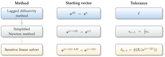
Figure 2.
Starting vectors and tolerances of the iterative methods.
The choice of the starting vectors is made so to start as close as possible to the solution of the system. Moreover, it also allows to write conveniently the linear system arising at each Newton iteration (e.g., see [16]). The stopping criteria, on the other hand, descend directly by the description of the LDM and by the choice of an inexact Newton iteration to solve the inner systems.
The starting vectors determine also the initialization of the tolerances: for example, at the first Newton iteration of the -th lagged iteration, the tolerance of the linear solver is . We can also easily notice that all the tolerances are initialized at at the first lagged iteration.
However, if we do not apply any correction, the initial tolerance of the linear solver, , may become smaller than the minimum possible tolerance of the simplified Newton method, . Thus, would be smaller than what could be required by an inexact Newton method, leading to an increase in computational cost with no foreseeable improvement in accuracy.
To avoid this situation, we simply impose as the minimum acceptable tolerance of the linear solver:
This does not lead to a worsening of the accuracy of the lagged procedure (indeed, is the tolerance of the simplified Newton method), while significantly reducing the computational cost.
4.3. Summary of the Solution Method
The diagram in Figure 3 summarizes the equations and the systems that we used, illustrating how the partial differential equation is first transformed in a system of ordinary differential equations and then in a series of nonlinear algebraic systems, which are afterwards progressively linearized by the iterative methods.
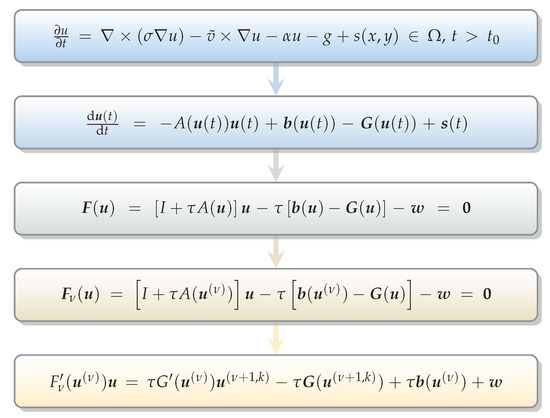
Figure 3.
Systems arising from the discretization of the initial PDE and from the used iterative methods.
Finally, we can write the algorithm summarizing the entire procedure as follows.
| Algorithm 1 Lagged diffusivity procedure | |
| Require: initial condition at ; a tolerance | |
| 1: for do | Time level |
| 2: Initialize solution vector for lagged iteration: | |
| 3: Initialize lagged tol.: | |
| 4: for do | Lagged iteration |
| 5: Initialize linear solver tol.: | |
| 6: for do | Simpl. Newton iteration |
| 7: for do | Linear solver iteration |
| 8: Compute -th iterate | |
| 9: Compute residual of the linear system | |
| 10: if then break | |
| 11: j = j+1 | |
| 12: end for | |
| 13: Compute Newton residual | |
| 14: if then break | |
| 15: Update linear solver tol.: | |
| 16: k = k+1 | |
| 17: end for | |
| 18: Update vectors and matrices: find | |
| 19: | |
| 20: | |
| 21: if then return | |
| 22: end for | |
| 23: | |
| 24: end for | |
Here, break means that we exit the current loop and go back to the outer one. On the other hand, return means that we exit from the entire procedure and the algorithm returns the final result. If the smoothness assumptions in Section 3.2 are satisfied (and if the inner linear solver converges), then the convergence of Algorithm 1 is ensured by Theorem 2 or by analogous theorems, depending on the chosen discretization.
5. Numerical Experiments
We consider a square domain , which we discretize by a uniform grid of inner points. We build test problems from known solutions (specified in the following) by computing an appropriate source term. When not otherwise specified, time discretization is performed by a method with and and we compute the solution from a starting time to a final time .
In the test problems we choose , and , which has the form of the radiation model. We instead consider several different choices of and of .
The linear systems arising at each Newton iteration are solved considering Krylov and splitting methods. In particular, we use the Preconditioned Conjugate Gradient (PCG) method [18] when the coefficient matrix of the linear system is symmetric and positive definite (i.e. = ). Here, the used preconditioner is the diagonal matrix M whose elements are given by the -norm of the i-th row of the coefficient matrix of the linear system. We instead compare the AM method [14] and the BiConjugate Gradient-stabilized method with parameter l (BiCGstab(l)) [19] when ≠ .
We choose ; the other stopping criteria are determined as in Section 4. The maximum number of simplified inexact Newton iterations is and the maximum number of linear iterations is . In the following subsections, , and denote, respectively, the total number of lagged, Newton and linear solver iterations required for computing the solution at the last time level. By and we instead denote, respectively, the initial residual and the last residual of the linear system at the last time level, while and rel. denote the global error (in and in relative Euclidean norm respectively).
5.1. Effect of the Discretization Scheme
Let us analyze the effect of the space discretization. In Table 1 we report the results obtained for different choices of with . We set ; with this choice, Equation (7) is satisfied for .

Table 1.
Comparison between discretization by central finite differences and by upwind scheme.
In Table 1, we see that the two discretization schemes are identical for = , also in terms of global errors and number of iterations. Indeed, in this case, the first-order derivative in the differential equation is multiplied by a null term. Thus, is symmetric positive definite and the two discretizations are equivalent.
In the other cases, both methods always work properly when respects the spacing condition, although global errors are larger when we use the upwind discretization. As mentioned above, this is to be attributed to the discretization of the first-order derivative by forward or backward finite difference quotients, leading to a larger discretization error.
Lastly, when the spacing condition is not respected anymore, we can have problems in the solution of the linear system. Indeed, the convergence of the AM method requires that the coefficient matrix is an M-matrix. Although the AM still works for values of for which this is not satisfied (e.g., ), we soon have problems for larger values of the velocity term. For example, (and any other larger velocity term) leads the AM to stall. Also the BiCGstab(1) presents some problems and it already stalls for . Contrary to the AM, however, the BiCGstab(1) does not explicitly require that the coefficient matrix is an M-matrix. Its stalling is, however, not surprising. Indeed, the BiCGstab(1) (which is equivalent to the BiCG-STAB [20]) is known for stalling especially when the coefficient matrix is real but its eigenvalues are complex with large imaginary part. This could certainly be the case, since, irrespective of the chosen discretization, the coefficient matrices are non-symmetric when . Complex eigenvalues are, thus, possible.
Then, it is interesting to see what happens increasing l in the BiCGstab(l) method. Indeed, l has been introduced exactly to overcome these difficulties. Let us then consider yet larger values of and analyze what happens using BiCGstab(2) and BiCGstab(4) as well. The results are reported in Table 2.
Table 2.
Comparison between discretization by finite differences and by upwind scheme with high .
As we expected, the AM and the BiCGstab(1) are not able to solve the linear systems arising when is large and central FD are used. Indeed, they stall and the maximum number of allowed linear iterations is reached. On the other hand, if the discretization is performed by an upwind scheme, the AM method always converges without presenting any problem (on the contrary, the algorithm gets faster with larger values of ). This was to be expected, since the coefficient matrix is now an M-matrix, as required by the convergence of the AM method. The BiCGstab(1), instead, keeps stalling for large values of , as we could expect from what we said in the previous paragraph. However, we can see that this can be overcome by increasing the parameter l of the BiCGstab(l): the algorithms using BiCGstab(2) or BiCGstab(4), indeed, converge in all cases. We can also see the big difference between the global errors obtained when discretizing by central finite differences or by an upwind scheme. Indeed, they are in the order of for central finite differences and in the order of for the upwind scheme. However, it is also to be noted that the upwind scheme is much faster, especially when we use the AM as inner solver. Thus, we may opt for central finite differences with, for instance, BiCGstab(2) as linear solver if we require smaller errors, while we may choose an upwind method with AM if we require lower computational cost.
5.2. Blow-Up
We now apply the LDM to problems with blow-up and boundary layer solutions. In particular, we consider the solutions in Figure 4, where T denotes the blow-up time.
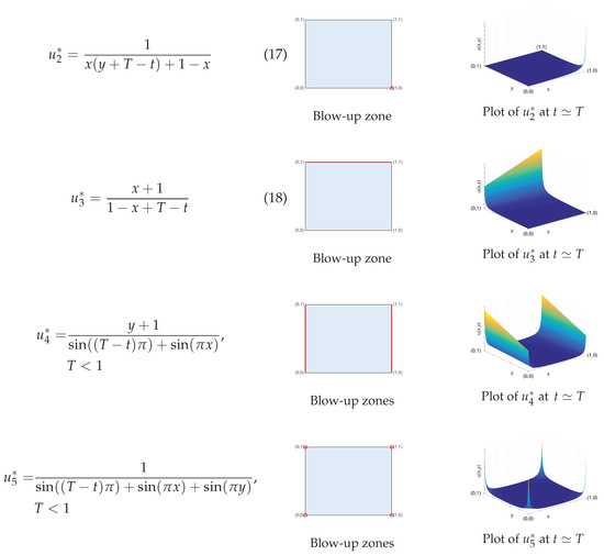
Figure 4.
Blow-up solutions and representation of where and how the blow-up occurs.
We set for and ; instead, and require by the periodicity of the trigonometric functions. In these two cases we therefore set .
With no loss of generality, the velocity vector is here set equal to zero and the system matrix is a Stieltjes matrix. We thus use the PCG solver for solving the linear systems arising at each Newton iteration and discretize space by central finite differences.
In the following results, denotes the maximum of the computed solution vector at the last computed time level, while denotes the maximum of the analytical solution at the last computed time level in the point where occurs. Analogously, we define and .
5.2.1. Preliminary Results and Analysis
Let us first analyze how the computed solution evolves as the blow-up time approaches. To this end, let us start from and see what happens at different times, until reaching T; at first, we here choose and . In Figure 5 we report what we get considering e.g., (example of solutions with blow-up on one corner), (example of solutions with blow-up on one or more edges) and (example of solutions with blow-up on more corners). In Table 3 we report some information on errors and data of the iterative procedure.
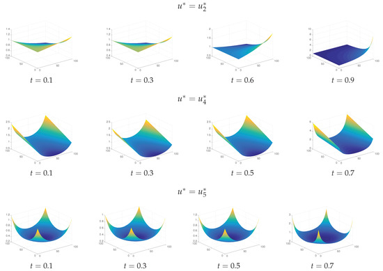
Figure 5.
Evolution of the computed solution as t approaches T in the cases , and .
Table 3.
Error and data of the lagged diffusivity procedure for , and as t approaches T.
Of course, in all these cases, the iterative procedure stops when we are still quite far from the blow-up time: indeed, using , the last computable time step is at when and when . Indeed, the blow-up occurs at and at respectively. We therefore need a smaller time step in order to get closer to the singularity. However, we notice that the computed solutions behave as the analytical ones (as proven by the errors in Table 3) and that, as the blow-up time approaches, they get more and more similar to the ones in Figure 4.
It is also interesting to notice that the residual computed at the beginning of the lagged iteration, , gets larger as we get closer to T. This can be viewed as an indicator of incoming blow-up: indeed, by the initialization , at the time step we have . Therefore, is the residual of as in (9) for at time . So, if the solution is smooth in the time variable (and is not excessively large), we do not expect to be large: in these hypotheses, the solution will not be dramatically different from the solution . However, if we have a singularity at some time T, the solution vector will change faster and faster as we approach T, leading to progressively larger initial residuals . In this light, the analysis of gives information similar to the analysis of the derivative of with respect to t.
5.2.2. Effect of Refining the Time Grid
Taking into account the previous results, let us set . We now start our analysis from , so that we do not need an extremely large number of iterations in order to get close to the blow-up zone.
In Figure 6 we show how the computed solution looks like at the last computable time step before the blow-up; we call this final time. In Table 4 we report some data on the lagged iterative procedure at .
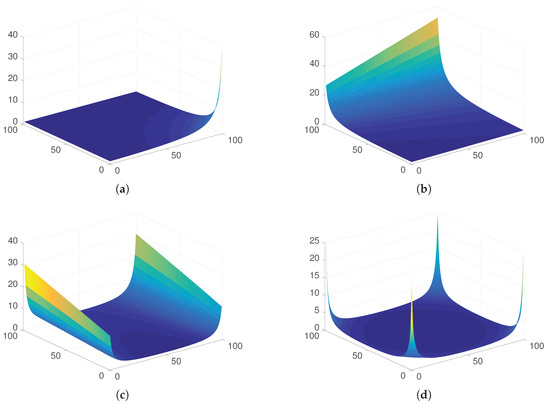
Figure 6.
Last computed solution for the problems in Figure 4 for . (a) , ; (b) , ; (c) , ; (d) , .
Table 4.
Error and data of the lagged diffusivity procedure for the last computable solution for the problems in Figure 4 for .
The first thing we notice is the extremely large values of , which are even more remarkable considering that has been reduced. This can be explained as in the previous paragraph by considering that the solution changes more and more rapidly as we approach T. A gradual increase of with t is indeed what can be observed by considering the value of at different time levels.
The analysis of the plots reveals that the lagged diffusivity procedure is able to reproduce the behavior of all the solutions near their respective blow-up zones. On the other hand, the global errors gradually increase, but they generally remain in the order of . Indeed, only for they exceed near T.
Notwithstanding this, maximum and minimum values of the solution vector correspond to the maximum and minimum values of (computed in the inner grid points) to at least the second decimal digit in all the cases. It is to be noticed that the maximum of is the point where the solution is nearest to the blow-up one; a good precision in evaluating the solution in this point is thus important for accurately reproducing the blow-up behavior.
Finally, we also notice that these maxima and minima of are not so large after all: we are near to the blow-up time, but the maximum of the solution never exceeds values , nonetheless. This cannot be explained by numerical errors in the solution procedure, since we said that the maximum of the computed is really similar to the value of in the grid point where the maximum occurs. Different causes concur to this:
- the blow-up occurs on the boundary, where the solution is given by the Dirichlet boundary conditions. Thus, at inner points, where we compute the solution vector, the maximum of is always smaller than the maximum of at boundary points when ;
- as a consequence of the previous point, the smaller the number of grid points, the smaller . Indeed, we get farther from the boundary and, thus, from the singularity. This is also shown in the next subsection, where we observe that increases when we increase the number of points of the space grid;
- the singularity occurs abruptly when is reached, so the solution is still quite small also at times quite close to T. Next, we show that by further reducing , we are able to get nearer to T, leading to an increase of .
All these facts can be better viewed by considering a short example. Let us consider and . We remind that the blow-up here occurs at in the point . The solution at at the inner point closest to , which is is:
as computed.
The algorithm, then, does not stall due to large values of , but because its derivatives become large. Indeed, considering the largest first-order derivative in x, we have
This makes so that the bound on backward difference quotients increases as the blow-up approaches. Then, it is harder to satisfy the monotonicity condition of Theorem 1, which, in turn, affects the uniqueness of the solution and the convergence of the LDM. We can try to counterbalance the larger by reducing (and, thus, , which appears in the condition of Theorem 1), as we verify in the next subsection. However, further decreasing means increasing the number of time levels and, thus, the computational time. Nonetheless, we can compensate this effect by starting our computations nearer to the blow-up time.
5.2.3. Effect of Refining the Space Discretization
Let us then analyze what happens when the space grid is refined; in this regard, the results obtained with and are reported in Table 5.
Table 5.
Error and data of the lagged diffusivity procedure for the last computable solution for the problems in Figure 2 for and .
We notice that slightly decreases, while the maximum and the minimum of in are about the same as previously computed for . Indeed, being the grid finer, the point nearest to the blow-up point is closer (in space) to the blow-up point than in the case . Thus, the solution gets larger earlier.
To better see this, we can again consider the short example proposed earlier and analyze what happens for . Let us again consider with in the point . The solution at at the inner point closest to , which is is:
as computed. Analogous results can be easily verified with regard to the derivatives. We also notice that global errors decrease due to the finer space grid, while is of the same order of magnitude as above.
Lastly, we verify that further reducing allows us to better approach the blow-up time, as remarked at the end of the previous subsection. Thus, in Table 6 we report the results obtained by setting and by using as the last computed time step of Table 5.
Table 6.
Error and data of the lagged diffusivity procedure for the last computable solution for the problems in Figure 4 for , .
In all cases we are able to get closer to the blow-up time, as expected. Moreover, global errors decrease.
5.3. Boundary Layer
Lastly, for completeness, let us consider a stationary case with non-constant which presents a boundary layer solution.
Let us consider the problem given by
and
with real parameter and boundary condition on . The solution of this test problem is evidently
which presents a boundary layer as the absolute value of increases. Since we do not have any nonlinear reaction term, at each iteration of the LDM we just have to solve a linear system, which we do by the BiCGstab(l) algorithm.
Table 7.
Analysis of a boundary layer example as increases (boundary layer occurs for large ).
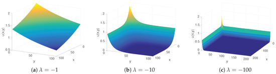
Figure 7.
Solution of the boundary layer test problem for N = 250; inner solver: BiCGstab(4).
We notice that the number of iterations of the linear solver decreases as increases. The global errors, instead, increase, but they never get larger than , confirming the good approximation of the solution. In particular, Figure 7c, correctly reproduces the profile of a boundary layer solution.
6. Conclusions
We analyzed the effect of the discretization on the LDM for the solution of nonlinear, non-steady convection-reaction-diffusion equations. Some insights on an efficient implementation of the algorithm are provided and are followed by numerical experiments, which highlight the differences arising when the space discretization is performed by central finite differences or by the upwind method.
The paper is completed by a numerical study on the application of the LDM to problems characterized by blow-up and boundary layer solutions. The numerical experiments show that the LDM is able to correctly reproduce the analytical solution also in proximity of the blow-up time or in presence of a boundary layer.
Author Contributions
The two authors contributed equally to both the theoretical and experimental parts of the work presented in this paper. They elaborated and discussed the results together at all stages of the preparation of the manuscript, which they wrote and revised jointly.
Conflicts of Interest
The authors declare no conflict of interest.
References
- Meyer, G. The numerical solution of quasilinear elliptic equations. In Numerical Solution of Systems of Nonlinear Algebraic Equations; Byrne, G., Hall, C., Eds.; Academic Press: New York, NY, USA, 1973. [Google Scholar]
- Galligani, E. Lagged diffusivity fixed point iteration for solving steady-state reaction diffusion problems. Int. J. Comp. Math. 2012, 89, 998–1016. [Google Scholar] [CrossRef]
- Ding, J. Blow-up solutions for a class of nonlinear parabolic equations with Dirichlet boundary conditions. Nonlinear Anal. Theor. 2003, 52, 1645–1654. [Google Scholar] [CrossRef]
- Ding, J.; Wang, M. Blow-up solutions, global existence and exponential decay estimates for second order parabolic problems. Bound Value Probl. 2015, 2015, 160. [Google Scholar] [CrossRef]
- Ding, J.; Hu, H. Blow-up and global solutions for a class of nonlinear reaction diffusion equations under Dirichlet boundary conditions. J. Math. Anal. Appl. 2016, 433, 1718–1735. [Google Scholar] [CrossRef]
- Protter, M.H.; Weinberger, H.F. Maximum Principles in Differential Equations; Springer: New York, NY, USA, 1984. [Google Scholar]
- Pucci, P.; Serrin, J. The Maximum Principle; Birkhauser Verlag AG: Basel, Switzerland; Boston, MA, USA; Berlin, Germany, 2007. [Google Scholar]
- Wang, Y.; Mu, C. Blow-up and scattering of solution for a generalized Boussinesq equation. Appl. Math. Comp. 2007, 188, 1131–1141. [Google Scholar] [CrossRef]
- Abia, L.; Lopez-Marcos, J.; Martinez, J. The Euler method in the numerical integration of reaction-diffusion problems with blow-up. Appl. Numer. Math. 2001, 38, 287–313. [Google Scholar] [CrossRef]
- Galaktionov, V.A.; Vazquez, J.L. The problem of blow-up in nonlinear parabolic equations. Discret. Contin. Dyn. Syst. 2002, 8, 399–433. [Google Scholar]
- Varga, R. Matrix Iterative Analysis, 2nd ed.; Springer: Berlin, Germany, 2000. [Google Scholar]
- Ortega, J.; Rheinboldt, W. Iterative Solution of Nonlinear Equations in Several Variables; Classics in Applied Mathematics; SIAM: Philadelphia, PA, USA, 2000. [Google Scholar]
- Isaacson, E.; Keller, H.B. Analysis of Numerical Methods; John Wiley & and Sons: New York, NY, USA, 1966. [Google Scholar]
- Ruggiero, V.; Galligani, E. An iterative method for large sparse linear systems on a vector computer. Comput. Math. Appl. 1990, 20, 25–28. [Google Scholar] [CrossRef]
- Rheinboldt, W. Methods for Solving Systems of Nonlinear Equations, 2nd ed.; CBMS-NSF Regional Conference Series in Applied Mathematics; SIAM: Philadelphia, PA, USA, 1998. [Google Scholar]
- Mezzadri, F.; Galligani, E. A Lagged Diffusivity Method for Reaction-Convection-Diffusion Equations with Dirichlet Boundary Conditions. Available online: http://www.nau.unimore.it/ANM-2017.pdf (accessed on 1 Auguest 2017 ).
- Dembo, R.S.; Eisenstat, S.C.; Steihaug, T. Inexact Newton Methods. SIAM J. Numer. Anal. 1982, 19, 400–408. [Google Scholar] [CrossRef]
- Hestenes, M.R.; Steifel, E. Methods of conjugate gradient for solving linear systems. J. Res. Natl. Bur. Stand. 1952, 49, 409–436. [Google Scholar] [CrossRef]
- Sleijpen, G.L.G.; Fokkema, D.R. Bicgstab(l) for linear equations involving unsymmetric matrices with complex spectrum. Electron. Trans. Numer. Anal. 1993, 1, 11–32. [Google Scholar]
- Van der Vorst, H. Bi-CGSTAB: A fast and smoothly convergent variant to the Bi-CG for the solution of nonlinear systems. SIAM J. Sci. Stat. Comp. 1992, 13, 631–644. [Google Scholar] [CrossRef]


© 2017 by the authors. Licensee MDPI, Basel, Switzerland. This article is an open access article distributed under the terms and conditions of the Creative Commons Attribution (CC BY) license (http://creativecommons.org/licenses/by/4.0/).