Abstract
In this paper, a robust technique based on a genetic algorithm is proposed for estimating two-view epipolar-geometry of uncalibrated perspective stereo images from putative correspondences containing a high percentage of outliers. The advantages of this technique are three-fold: (i) replacing random search with evolutionary search applying new strategies of encoding and guided sampling; (ii) robust and fast estimation of the epipolar geometry via detecting a more-than-enough set of inliers without making any assumptions about the probability distribution of the residuals; (iii) determining the inlier-outlier threshold based on the uncertainty of the estimated model. The proposed method was evaluated both on synthetic data and real images. The results were compared with the most popular techniques from the state-of-the-art, including RANSAC (random sample consensus), MSAC, MLESAC, Cov-RANSAC, LO-RANSAC, StaRSAC, Multi-GS RANSAC and least median of squares (LMedS). Experimental results showed that the proposed approach performed better than other methods regarding the accuracy of inlier detection and epipolar-geometry estimation, as well as the computational efficiency for datasets majorly contaminated by outliers and noise.
1. Introduction
Sparse image matching is one of the most critical steps in many computer vision applications, including structure from motion (SfM) and robotic navigation. In contrast to dense image matching, where image correspondences are established at nearly each pixel, sparse matching establishes the correspondences at salient image points only. Recent research works apply sparse matching to address a variety of problems including simultaneous localization and mapping [1,2], feature tracking [3] and real-time mosaicking [4,5]. The results of sparse matching are usually contaminated with false correspondences. Given the recent advancements in the fields of low-altitude, oblique and ultra-high resolution imagery, the rate of contamination has increased, and detecting the correct correspondences with high accuracy has become more challenging [6]. This is due to several factors, which include noisy measurements, the inefficiency of local descriptors, the lack of texture diversity and the existence of repeated and similar patterns that cause matching ambiguity [7,8,9]. Therefore, outlier detection should be substantially integrated into sparse matching. From now on, the term putative correspondence is used for referring to the raw results of sparse matching. The term inlier applies to true matches among the putative correspondences, and the term outlier refers to false matches. Besides, the terms correspondence and match have the same meanings throughout this paper. The problem of outlier detection implies the detection of inliers by eliminating outliers from putative correspondences given no prior information about the parameters of relative orientation or intrinsic camera calibration assuming straight line-preserving perspective camera models.
Outlier detection techniques are based on the fact that inliers have some spatial characteristics in common. The correspondences that are not consistent with such spatial characteristics can be classified as outliers. The idea of using epipolar geometry as a spatial constraint to detect inliers/outliers has been proposed in several studies. In this regard, the outlier detection problem turns into two problems of (i) robust estimation of epipolar geometry given the putative correspondences and (ii) detecting all of the inliers and outliers using the estimated model. In this paper, the term model refers to the two-view epipolar geometry, which is described here by the fundamental matrix. In particular cases where approximations can be made on the perspective camera model or assumptions can be formulated about the planarity of the scene, the model can refer to affine transformations and homographies, as well. Figure 1 presents the summary of the outlier detection techniques that are discussed in Section 2. In addition to the techniques using epipolar geometry, several methods are based on other spatial criteria, such as the distribution of parallax values [10,11], spatial patterns of outliers [12], orientations of the lines connecting inliers [13] and two-way spatial order differences [14]. However, such methods use spatial consistency measures that are less general and valid for specific imaging configurations.
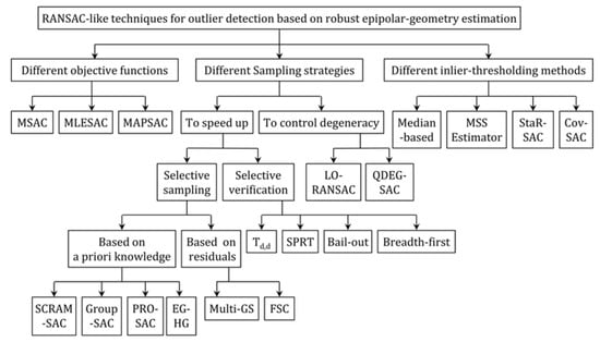
Figure 1.
Summary of outlier detection techniques in stereo sparse matching based on robust estimation of epipolar geometry.
In this paper, we also focus on the problem of outlier detection based on the robust estimation of epipolar geometry. To this end, we use the integer-coded genetic algorithm (GA) followed by an adaptive inlier-classification method. The proposed technique can be considered as an extension and generalization of RANSAC-like methods for handling a high percentage of outliers, varying amounts of noise and degenerate configurations. This technique has the following distinctive characteristics. First, random sampling is replaced with an evolutionary search. The evolutionary search brings a significant advantage: new sample sets are generated considering the feedback information obtained by evaluating previous sample sets. Second, a guided sampling scheme based on the spatial distribution of the correspondences is proposed and applied to the evolutionary search. This sampling scheme increases the robustness of the solutions against degenerate configurations and local optima without requiring additional computation or prior information about the matches. Third, the objective function of robust estimation is not defined based on the support cardinality, but the robust least trimmed sum of squared residuals is used instead. Therefore, there is no need to successively set a threshold at any iteration for detecting the support of the estimated model or to assume any specific probability distribution for outlier/inlier residuals. Finally, to identify all of the inliers, a detection method based on adaptive thresholding is proposed, as opposed to using a fixed threshold. In this approach, the uncertainty of the estimated model is taken into account to identify all of the inliers correctly.
The rest of the paper is organized as follows. In Section 2, a review of the techniques of robust epipolar-geometry estimation is presented. The main problem of simultaneous inlier detection and epipolar-geometry estimation is formulated in Section 3. Section 4 describes the solution using the genetic algorithm, which is followed by the method of detecting all of the inliers. The experimental results are discussed in Section 5, and the conclusion is presented in Section 6.
2. Related Works
Random sample consensus (RANSAC) techniques are popular approaches in fields of robust estimation [15]. RANSAC is a method to estimate the parameters of a mathematical model from a set of observations that contain outliers, assuming that the quality of the model and the observations are inter-dependent. More precisely, RANSAC aims at determining the optimal model from an outlier-free sample set of correspondences by maximizing the support size of the model. The inliers that support the model are detected as correspondences whose residuals from the estimated model are less than a given threshold. To find an outlier-free sample set, successive random sampling is performed. To ensure, with probability p, that at least one outlier-free set of m correspondences is drawn from a dataset containing percent of inliers, at least k sample sets should be drawn such that . This also means that within RANSAC, approximately, good models are generated before the confidence p is achieved.
By this definition, six major questions are involved in RANSAC-like techniques. (i) Is maximizing the support cardinality a robust objective function when no information about the rate of the outliers is available? (ii) How does one handle a large number of required samples in cases where is very small? (iii) Why does the algorithm not take advantage of the probability of generating good hypotheses before reaching the termination criterion; i.e., why not include the feedback of previous samples in the sampling procedure? (iv) How can the robustness of the estimated model be ensured against the influence of noise since it is relying on a minimal (just enough) subset of inliers? (v) How does one control the effect of degenerate sample sets, which naturally maximize the support cardinality? (vi) Does the threshold used to detect the inliers reflect the uncertainty of the estimated model as well? Some of these questions are answered by different variants of RANSAC, which are discussed here.
Unlike the standard RANSAC, there are improved variants, which use robust objective functions to determine the support cardinality. In m-estimator sample consensus (MSAC), inliers are scored based on their fitness, and outliers are scored with a non-zero constant penalty [16]. Maximum likelihood estimation sample consensus (MLESAC) maximizes the log-likelihood of the solution via the RANSAC process by assuming that outliers are distributed uniformly and residuals distribute a Gaussian function over inliers [17]. Maximum a posterior estimation sample consensus (MAPSAC) is also a refined version of MLESAC with Bayesian parameter estimation [18]. These objective functions make models with similar inlier scores more distinguishable. However, they make certain assumptions about the distribution of the residuals either for inliers or outliers. Besides, they still score the models and detect the final inliers by applying a hard threshold to the residuals. Generally, this threshold is determined from the standard deviation of the residuals themselves. Assuming that the noise in data points follows a Gaussian distribution and that the residuals are expressed as point-model distances, then the residuals follow a Chi-square distribution. Therefore, the threshold can be expressed as , where is the cumulative Chi-square distribution with one degree-of-freedom at probability p as the fraction of the inliers to be captured (e.g., ). However, this assumption is valid when ignoring the uncertainty of the model itself. Besides, estimating the standard deviation at any RANSAC iteration is another problem. One of the most common methods is to estimate this variable from the median of the residuals on the potential inliers that support the best tentative model. Therefore, it might not be robust against outliers [19]. Another method is to determine a Gaussian distribution fitting to the smallest residuals in the dataset (modified selective statistical estimator (MSSE) by [20]). While this method is more robust against outliers, it is sensitive to the distinction of inliers from outliers. One strategy to eliminate the requirement of a fixed threshold is to run RANSAC several times using a range of pre-determined thresholds (the stable random sample consensus (StaRSAC) method by [21]). However, depending on the range of the thresholds to be tested and the number of RANSAC executions, this strategy can be computationally exhaustive. In the RANSAC with uncertainty estimation (Cov-RANSAC) algorithm, the uncertainty of the model estimated from the minimal sample set is used to determine a subset of potential inliers, to which the ordinary RANSAC is applied afterwards [22]. However, the uncertainty of the estimated model highly depends on the uncertainty of the configuration of the points appearing in the minimal sample set.
The sampling strategy in RANSAC is also an important factor, as it influences the algorithm efficiency with respect to both the number of RANSAC iterations and degeneracy (Degeneracy in robust epipolar-geometry estimation occurs when one or more degenerate configurations exist in the scene. This usually happens when the majority of the correspondences belong to a dominant plane in the scene and the rest of the correspondences are not on the plane (planar degeneracy), or when the correspondences belong to a very small region of an image (ill-configuration).) of the estimated model. There are several methods to control each of these two factors. The main contributions in this regard are discussed here. To control the speed of the algorithm, two strategies can be applied. The first strategy is to enforce an initial consistency check to filter the putative correspondences. This consistency can be measured as the fraction of neighbouring features in a region around a point in one image whose correspondences fall into the similar region in the other image (Spatially Consistent Random Sample Consensus (SCRAMSAC) method by [23]). This strategy is sensitive to the region size and the threshold used to define the spatial consistency. Alternatively, sampling can be guided by keypoint matching scores (Progressive Sample Consensus (PROSAC) method [24], Efficient Guided Hypothesis Generation (EGHG) method by [25]). However, such a strategy is not effective when foreground motion happens. In addition, the scenes with repetitive textures may result in many false matches with high matching scores. Another example of such strategies is to assume that correspondences have a natural grouping structure, in which some of the groups have higher inlier probability than others (the GroupSAC method by [26]). However, finding a meaningful and efficient grouping among the correspondences is itself a concerning challenge in different applications.
The strategies mentioned so far mostly require supplementary information about the scene or the matches. Comparatively, guided sampling based on the information from sorted residuals can be used to accelerate the hypothesis generation while avoiding any application-specific ordering or grouping technique (Multi-Structure Hypothesis Generation (Multi-GS) by [27]). In this method, sampling is guided towards selecting the points that are rising from the same structure. This strategy speeds up the procedure to reach an outlier-free sample set. However, this method causes more computational complexity, since every point in the hypothesized sample set should be compared against all of the other points in the dataset in order to determine its intersection (in terms of structure) with them. The fast consensus sampling (FCS) method based on the residuals is developed by [28]. In this method, proposal probabilities are calculated for the correspondences based on their normalized residuals and a concentration score. Although this method accelerates the sampling, it is still sensitive to degeneracy, image noise and uncertainty of the model estimation. This is due to the fact that it reduces the number of potential inliers by thresholding the proposal probabilities that are, themselves, dependent on the robust estimation of normalized residuals. Several studies have attempted to apply evolutionary algorithms instead of the random search [29,30]. Although promising results were achieved, several limitations were not addressed yet. For instance, their objective functions still require a hard threshold to distinguish outliers from inliers; the two-dimensional spatial configuration of the correspondences is ignored; the uncertainties of the estimated model are not taken into account; and the experiments are limited to small datasets. Genetic Algorithm Sample Consensus (GASAC) is also another technique that is, to the best of the authors’ knowledge, the most similar technique to the one proposed in our study. The difference of GASAC from typical RANSAC is that the random sampling is replaced with evolutionary search based on classic genetic algorithms (genetic algorithms are meta-heuristics inspired by biological evolution, which are used for solving optimization problems by relying on evolutionary search operators) [31]. This study shows that the computational cost could be sped up 13-times by applying the evolutionary search instead of the random one. However, according to their report, the technique is applicable to small datasets with less than 50% outliers; the objective function is still based on support cardinality; and it introduces no solution to avoid local optima (such as degeneracy). The second strategy proposed in the literature in order to speed up RANSAC is to reduce the solution space by only verifying the hypotheses with a higher probability of being optimal. These highly probable hypotheses can be selected by a test [32], a bail-out test [33] or a sequential probability ratio test (SPRT) [34,35]. In addition, the hypothesis verification can be performed preemptively in a breadth-first manner only for a fixed number of sample sets [36]. These techniques may increase the number of required hypotheses, as good models may wrongly be rejected by not being verified completely.
It has been observed that, in the case of degenerate configurations, RANSAC-like algorithms result in a model with a very large support, while it is completely incorrect. This behaviour can be explained by the fact that a high inlier support can be obtained even if the sample set includes some outliers and at least five inliers that belong to a dominant plane or to a very small area of the image. This large support causes the termination of RANSAC before a non-degenerate outlier-free sample set can be picked up [37]. The main strategy to control the degeneracy of solutions is to re-investigate the support of the best tentative model either locally or globally. For instance, the support of the best model can be re-sampled, and the model estimated from those subsamples can be compared to the best one to find out the degenerate models (the Locally Optimized Random Sample Consensus (LO -RANSAC) method by [38]). Another example of such strategies is the Quasi Degenerate Sample Consensus (QDEGSAC) (proposed by [39]), where a hierarchical RANSAC is performed by changing the number of the parameters in the model and verifying it over the entire dataset. The main issue concerning these techniques is that they cause additional operations, as a separate mechanism is added to the original RANSAC; i.e., they do not directly handle degeneracy in the sampling process. Universal RANSAC (USAC) is also a modular fusion of some of the mentioned RANSAC algorithms, including PROSAC sampling, SPRT verification and LO-RANSAC local optimization [40]. In general, its performance is better than any of the single modules integrated into the universal implementation. However, it does not improve any of the modules individually.
To conclude, in most variants of RANSAC, the termination criterion is decided based on the size of the maximum consensus set found, which itself depends on the methods of threshold selection. These methods usually ignore the effect of the uncertainties of the estimated models caused by noisy image observations and spatial configurations of the matches in the minimal sample sets. Most RANSAC algorithms require extra operations or validations to increase the robustness of the results against degenerate configurations, and finally, they do not provide an explicit solution to maximize the accuracy of inlier detection.
3. Problem Formulation
In this section, the main problem of inlier detection is mathematically formulated. First, the fundamental theories of two-view epipolar geometry are explained, and our fast solution to this problem is presented. Then, a threshold-free objective function for robust estimation is formulated.
Notation: Column vectors are represented by italic, bold lower case letters, such as . Therefore, (the transpose of x) is a row vector. Matrices are denoted by italic uppercase letters, such as F. The elements of the matrix are denoted as , where i represents the row index and j represents the column index. Sets are denoted by italic, bold uppercase letters, such as .
3.1. Fundamental Theories: Two-View Epipolar Geometry
Epipolar geometry defines the geometry of stereo vision, all elements of which can be captured by a matrix called the fundamental matrix. It can also be captured by an essential matrix in the case of calibrated images, where the parameters of intrinsic camera calibration are known. There are different methods for estimating the fundamental matrix: linear, iteration-based and robust techniques [41]. Robust techniques, which use linear techniques as their base, are the most applicable ones since they can handle the presence of outliers and, finally, can detect the inlier correspondences required for structure reconstruction. This category of estimation is considered in this study. The following paragraphs present the theoretical background with this regard.
For any pair of homogeneous coordinates of correspondences in two images, the fundamental matrix (F) is defined by Equation (1).
It can be noticed that F is defined up to an unknown scale. It is also a rank-two matrix with zero determinant. Consequently, it has only seven degrees of freedom [42]. Given m matches , it would be possible to form a linear homogeneous system of equations in the nine unknown coefficients of matrix F as:
where , and matrix A is the coefficient matrix as . The coordinates of the points are also usually normalized so that A can gain a better condition number [43]. Given a pair of matching points with normalized coordinates and , the row corresponding to this match is defined as:
In robust estimation, non-parameterized linear methods of fundamental-matrix estimation are used due to the reasonable agreement between the speed and accuracy yielded from these methods [44]. Given exactly seven matches (), it would be possible to determine by spanning the two-dimensional nullspace of A and applying the rank deficiency constraint to it (seven-point algorithm). However, this results in up to three fundamental matrices. Thus, when the goal is the robust estimation of the fundamental matrix, computational expenses for hypothesis evaluation would increase up to three times. Depending on the total number of correspondences and the percentage of outliers, this can be a major drawback. Therefore, eight or more matches () are required to determine a single solution for the fundamental matrix (eight-point algorithms). Using at least eight points, the solution to F can be found from Equation (2) by linear least-squares methods. In the end, the rank deficiency constraint must be applied to the estimated F by setting its smallest singular value to zero [43].
In the case of the eight-point algorithm, an additional constraint should be imposed to define an arbitrary scale factor for F and to prevent the trivial solution . There are two options in this regard. One would be to fix the two-norm of the fundamental matrix (e.g., ). The other would be to fix one element of the matrix (e.g., ). In the first case (), an orthogonal least-square minimization should be applied. It can be shown that the solution is the right singular vector of A corresponding to the smallest eigenvalue of , which can be determined by singular value decomposition (SVD) of matrix A. Technically, to compute the SVD of the matrix , flops (amount of arithmetic operations) are at least required [45]. In the second case (), a set of non-homogeneous linear equations with equation matrix is produced, the solving of which requires m flops [45]. Therefore, applying the linear scale constraint () is computationally 13-times faster than the non-linear constraint for the minimal case of . In addition, it would be possible to add the observation weights directly and to use weighted linear least-squares techniques [46]. However, using this option is quite risky, as it influences the estimation of F if the coefficient approaches zero ([47]. Such situations () can be raised in cases that we will call poor camera models. In these cases, the above-mentioned assumption () fails; e.g., the rotation of the second camera coordinate system with respect to the first one is mainly planar, the camera motion contains pure translation or two cameras are only shifted along each other’s optical axes. A way to avoid such exceptions is to examine all nine elements of the fundamental matrix for setting them to a constant non-zero value (i.e., ) and choosing the best solution [48]. However, this increases the computational time.
In this study, Gaussian elimination with partial pivoting is used to detect the free variable of the consistent linear system of Equation (2) and to solve it. The free variable corresponds to the element of the fundamental matrix, whose corresponding column in the coefficient matrix (A) is not a pivot column. Therefore, that element cannot be zero and can take a fixed value, e.g., one, to resolve the scale deficiency of the fundamental matrix. In terms of complexity, partial pivoting requires flops. Therefore, its application is not efficient for large datasets. However, in the case of robust estimation where only a minimal number of eight points is used, this method requires only 341 flops (compared to 9351 flops for SVD decomposition).
Given an estimated fundamental matrix, it is possible to express how well the correspondences fit to it by calculating the residuals of the correspondences [19]. There are various error measures to represent the residuals, including algebraic distance, epipolar-weighted distance, two-sided point to epipolar line distance and the Sampson distance:
where and . The ideal measure for robust estimation should not be highly sensitive to image noise. As the previous studies have shown, the Sampson distance is less sensitive to image noise in comparison with other error measures. Therefore, the Sampson distance is used in this study to represent the residuals.
3.2. Robust Estimation Problem
The main problem of robust estimation is to find a minimal sample set of inliers, from which the fundamental matrix (the model) can be estimated correctly. To determine how correct an estimated model is, an objective function is required. In RANSAC robust estimation, this objective function is defined as the support of the estimated model. However, as mentioned in Section 2, this requires a threshold to decide whether a correspondence supports the estimated model or not. In this study, to avoid such a threshold, the concept of least trimmed squares (LTS) [49] is applied. The objective is to minimize the sum of squared residuals over a minimum number of inliers, which we would call an inlier set of minimum cardinality denoted by . Given a candidate sample set of correspondences, a fundamental matrix, F, can be estimated via Equation (2). Therefore, the inlier set of minimum cardinality, , would be the set of correspondences with the smallest residuals, , leading to the cost function :
where . The cardinality of , , can be hypothesized without loss of generality. For instance, one can assume that, in a dataset containing 1000 putative correspondences, at least 100 matches are inliers without having any knowledge of the errors; i.e., . The minimum number of inliers would be a more relaxed assumption in comparison with the approximate ratio of outliers.
4. Robust Estimation via the Genetic Algorithm
In this paper, a modified version of the integer-coded genetic algorithm, originally proposed by [50] is applied to stochastically search for a sample set of correspondences that minimizes Equation (5). In GA terminology, each candidate sample set of correspondences is called an individual. The characteristics of an individual are represented by a chromosome. Each chromosome is made of a number of elements, called genes. In the context of this study, each gene accounts for a putative correspondence. Considering the minimal number of correspondences needed to find a solution for F, the length of a chromosome remains constant (e.g., eight points). A group of individuals, e.g., 30 ones, forms a population. The first step in applying the GA is to generate an initial population. The size of the population and the way its individuals are drawn (sampling strategy) are the most important factors to decide. Afterwards, in any iteration of the evolution, the model estimated from each individual is evaluated based on the objective function (Equation (5)). Then, the genetic reproduction operators are performed to reproduce a new population. This evolution continues the same way until reaching an optimal solution. The overall pseudo-code of the proposed technique is given in Algorithm 1.
| Algorithm 1: The proposed robust-estimation technique via the genetic algorithm. |
| Input |
| A set of n putative correspondences |
| Output |
| Estimated fundamental matrix and the entire set of inlier correspondences |
| (a) Genetic Algorithm |
| −Input: The lookup table of matches (Section 4.1) |
| −Output: The fundamental matrix (F) and an inlier set of minimum cardinality |
|
| (b) Estimate the uncertainty of the model () (Section 4.4) |
| (c) Estimate the average and uncertainty of the Sampson residuals () for matches belonging to to determine the outlying threshold (Section 4.4) |
| (d) Compute and threshold the Sampson residuals on other matches to identify the entire set of inliers (Section 4.4) |
4.1. Encoding
A significant step in the design of the GA is to find an appropriate representation of individuals, which is an encoding of candidate solutions to the problem as a chromosome. Assume that the input dataset contains n putative correspondences as (, ). Each correspondence has an index, k, which is given to it based on a random permutation of numbers from one to n. In previous studies (Rodehorst and Hellwich, 2006), the genes are directly defined as the index of each correspondence. However, GA operators take these integers as inputs to create new solutions. Therefore, these integers would better represent the correspondences in a way that makes geometrical or physical sense. To this end, in this study, each correspondence is labelled with a triplet of integers: one integer, k, as its index, as well as two integers, h and v, as the horizontal and vertical coordinates of the left point relative to the other points on the left image. In this study, the length of the chromosomes (the size of each minimal sample set) is set to 12. Therefore, each individual can be encoded as a sample set . Values and represent the vertical and horizontal dimensions of an overlapping rectangle, which is defined as the rectangle that minimally bounds all of the putative correspondences on the left image (Figure 2a). Note that the reason why the size of is set to 12 is explained in Section 4.2.
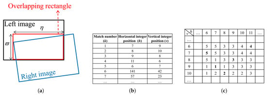
Figure 2.
Encoding scheme: (a) the overlapping rectangle, (b) an example list of some putative correspondences, which are identified by their indices, and their positions relative to the overlapping rectangle and (c) a part of the 2D lookup table constructed using Equation (6); the bold numbers show the indices of the original matches, and the regular numbers show the indices assigned to the other pixels.
Given this encoding, to reach the coordinates of the i-th gene inside an individual (i.e., ), the index is used. However, the genetic operators are applied to and . One may note that applying the genetic operators to and can result in new integers, where no correspondence might be located. To resolve this issue, a 2D lookup table is produced, by which an index is assigned to any empty pixel of the overlapping rectangle based on its proximity to the putative correspondences. In other words, the lookup table, T, finds the closest match to any arbitrary coordinates, (), inside the overlapping rectangle:
The lookup table in Equation (6) is identical to the indices in the Voronoi diagram of the points in the left image, measured with Manhattan distances. As an example, consider the matches in Figure 2b and their corresponding lookup table in Figure 2c. An instance of an encoded gene would be . Now, consider the application of the mutation operator to this gene. The mutation operator randomly changes the values of the genes. Assume that the application of the mutation operator to (indeed to values of and ) has resulted in new integers and . From the lookup table (Figure 2c), it can be seen that these integers correspond to . Therefore, the mutation operator changes to .
4.2. Sampling GA Individuals
The first step to initiate GA is to generate a random population of individuals. As mentioned in Section 3.1, at least eight points are required to form a minimal sample set from which the fundamental matrix can be calculated. As discussed in Section 2, random sampling can be either done uniformly or with an order based on the quality of the correspondences. However, none of these sampling strategies avoids degenerate configurations. To decrease the degenerate solutions, guided sampling based on the spatial distribution of the correspondences is proposed in this paper. To this end, first, the overlapping rectangle (shown in Figure 3a) is divided into 12 sub-regions of equal area as in Figure 3b. Then, the density of each region is calculated as the number of correspondences enclosed by it, normalized by the total number of correspondences.
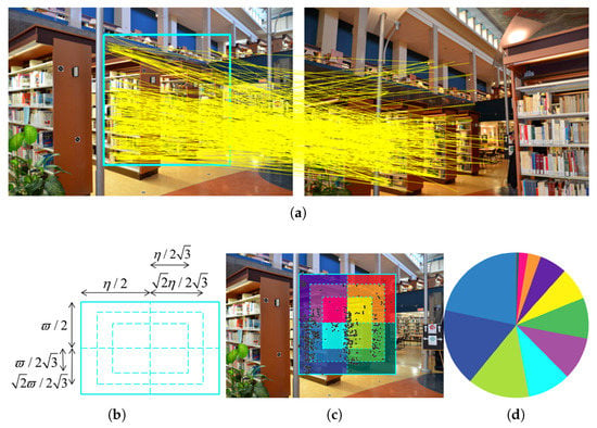
Figure 3.
Guided sampling: (a) a stereo pair and the putative correspondences; the bounding rectangle on the left image represents the overlapping rectangle; (b) dividing the overlapping rectangle into 12 sub-regions of equal area; (c) the minimal rectangle and the distribution of putative matches over the sub-regions; (d) density-based roulette-wheel for region selection.
For the first half of the population, the 12 correspondences are picked up from the regions that are selected successively in a roulette-wheel selection. The density of a region determines its probability to participate in sampling. In simple words, the wheel is turned 12 times, and every time, a region is selected from which to draw a match. For the other half of the GA population, every individual is made of twelve correspondences in a way that at least one match is sampled from each region. The reason for introducing this two-step sampling is to avoid high-density regions having full dominance in the population. Figure 3c illustrates an example of putative correspondences distributed on the overlapping rectangle, and the roulette wheel corresponding to it is shown in Figure 3d. Once the population is formed, the correspondences of every sample set in the population should be substituted into Equation (2) to determine the fundamental matrix (F). Then, each fundamental matrix is evaluated using the cost function in Equation (5), and its fitness is decided; the lower the value of the cost function, the fitter the individual.
The primary goal of the proposed scheme for subdividing the overlapping rectangle is to decrease the risk of sampling ill-configured points. Evidently, more than 12 sub-grids could be considered for sampling. However, the greater the number of points, the higher the risk of encountering outliers and the lower the probability of reaching outlier-free sample sets. Besides, 12 data points are already proposed by other studies such as [38,51]. Of course, there would still be a probability that the sampled points are too close to each other and cause ill-configurations. Such cases might especially happen when the points are selected from the regions close to the same edges or the same corners of the grid cells. It can be shown that the gridding scheme of Figure 3b is up to two-times more robust to this type of ill-configuration compared to a simple regular grid.
4.3. Genetic Operators
Once the individuals are evaluated, a selection operator is applied to the population to allocate the instances of fitter individuals for entering a mating pool as parents to reproduce a new generation (a generation in the context of genetic algorithms is equivalent to an iteration in the context of RANSAC). The tournament selection is used here due to its higher computational efficiency over other selection techniques [50]. Afterwards, new individuals are generated from the selected parents by applying crossover and mutation operators during a reproduction process. Crossover means creating two new individuals (called offspring) by combining two selected parents. Mutation means randomly changing the genes inside a chromosome. These procedures are explained below.
Let and be two selected parents. Furthermore, let the followings auxiliary variables be defined as and . The parameter is defined via Equation (7) in order to respect the bounds of correspondences on the images.
In Equation (7), includes two uniformly-distributed random numbers between zero and one, and . The crossover operator combines the two parents to produce two offspring, and , via Equations (8) and (9).
The mutation operation should be applied with caution to not highly distort sound solutions [52]. Furthermore, it should take into account the fact that usually inliers tend to be closer to each other than outliers (as assumed in the N Adjacent Points Sample Consensus (NAPSAC) robust estimation method by [53]). Therefore, mutation should perform a random local search for possibly finding more inliers in the vicinity of the currently-sampled points. A mutated solution, is created from a recently-produced offspring solution using Equation (10):
where and . In Equation (10), , includes two random uniformly-distributed numbers between zero and one; follows a power distribution with having random values between zero and one.
At any iteration, a random exploration is also performed by generating a fixed number of individuals based on the proposed guided sampling strategy in Section 4.2. Generating random solutions as a fixed portion of the population reduces the chance of converging to local optima.
The replacement strategy applied in this study can be considered as a combination of steady-state and elitist replacement methods. It helps to keep the best solutions from older generations and to maintain the population diversity to avoid premature convergence. Assume that is the population of the last generation, is the population of the selected parents from and is the population of the reproduced offspring using . Accordingly, demonstrates the least fitness value among the best third quartile of individuals in . Therefore, the new population starts forming by the fittest individuals of (elites). Among the elite individuals with similar fitness, those who are formed by correspondences coming from more distinct regions of the overlapping rectangle have priority in replacement. This way, the chance of ending with the local optima is highly reduced. In fact, this factor is used to distinguish models with similar fitness values. The rest of the spots available at are occupied by the following replacement condition:
where means the i-th individual in the population, . Equation (11) implies that an offspring whose quality is worse than 75% of the previous solutions is not qualified enough to replace its parents. The genetic algorithm iterates the procedures mentioned above until there is no improvement in the average of the elites’ fitness values during a specified number of generations.
4.4. Inlier Classification
Once the genetic algorithm terminates, the inlier set of minimum cardinality, , is found, and the final fundamental matrix, , is re-estimated using these points by performing iterative least squares adjustment using the Gauss–Helmert model as:
where the vector observations, , include the coordinates of correspondences, , , which are normalized by T and as Hartley normalizing transformation as such , . The vector of parameters is ; note that one element of the fundamental matrix, here , is assumed fixed based on the direct result of F obtained from the GA.
Now, inliers can be distinguished as the correspondences with residuals from that are less than a given threshold. The important issue would be determining this threshold. Standard RANSAC algorithms determine this quantity using maximum likelihood estimation based on the median of the residuals associated with the best tentative model. In this paper, the uncertainty of the final fundamental matrix is considered to calculate an adaptive threshold as follows. First, the covariance matrix of the estimated parameters can be derived using the covariance law as in Equation (13):
where and are Jacobian matrices calculated at re-estimated coordinates of the correspondences , and is the vector of estimated residuals. From Equation (12), . We can determine the uncertainty of the estimated fundamental matrix using the rules of error propagation as follows.
For each match belonging to the inlier set of minimum cardinality, the Sampson distance and its variance can be calculated via Equation (15).
The average of these distances, , and their standard deviation, , can represent the distribution of the residuals for inliers. Considering Chebyshev ’s inequality, at least 95% of the population is within -times the standard deviation from the mean, no matter what kind of probability distribution they are following. Therefore, every match with index j is an outlier by the confidence of 95% if its residual, , is greater than . To ensure a maximum set of inliers and avoid possible false positives or negatives, this whole procedure can be repeated a few times using the new set of detected inliers.
5. Experimental Results and Discussion
To demonstrate the efficiency of our algorithm and its individual components, we performed several experiments on simulated and real data. The variables that are tested with these experiments include: (i) the performance of our sampling scheme; (ii) the accuracy of our adaptive thresholding method for inlier classification; (iii) the effect of GA population size on the performance of the algorithm and (iv) the performance of the overall algorithm under different levels of noise, outliers and degeneracy. Table 1 summarizes the criteria used to assess these variables.

Table 1.
Criteria for performance assessment.
The experimental results obtained from the proposed technique are compared with those of the following state-of-the-art techniques: RANSAC, MSAC, MLESAC, LO-RANSAC (Lebeda et al., 2012), StaRSAC, Cov-RANSAC, Multi-GS-RANSAC and least median of squares (LMedS). Note that for implementing these techniques, the programs were prepared by the authors of this manuscript except for the following ones. The MATLAB built-in computer-vision toolbox was used for LMedS. For measuring the uncertainty of the fundamental matrix in Cov-RANSAC, the code was provided by the original authors [54]. The code for Multi-GS sampling was also provided by the authors [27].
5.1. Experiments on Synthetic Data
Several synthetic datasets were used to evaluate the performance of our algorithm. Using the synthetic data allowed us to control the imaging geometry, the fraction of outliers and the image noise. Besides, it let us assess the accuracy of inlier detection and model estimation in comparison with the ground-truth. Instead of creating random correspondences without having any particular geometric or physical form, real 3D point clouds were used to generate synthetic images. The synthetic outliers were produced in a relatively small range of error because large gross errors can be easily detected by statistical tests. Thus, we are interested in testing the performance of the proposed method in dealing with medium ranges of errors (smaller than 40 pixels). The synthetic datasets are described in Table 2. Different scenarios were chosen to cover diverse real-world cases including close-range and aerial photography, narrow and wide baselines and degenerate configurations. The following paragraphs briefly explain the reasons for which each dataset was selected for these performance tests.

Table 2.
Description of synthetic datasets.
The Table dataset: This is mainly generated to simulate a degenerate configuration, where a large number of correspondences is located on a planar object. Therefore, the performance of the sampling technique under degeneracies (Section 5.2.1) was tested on this dataset.
The Church dataset: This does not have any degenerate configurations. This close-range stereo-pair contains a small number of correspondences, which allows the application of the Multi-GS-RANSAC method. Furthermore, a low level of noise is simulated, which is usually the case of close-range images with static imaging platforms. The relative orientation of two cameras is quite challenging from the photogrammetric point of view (a narrow baseline and large relative rotations). Therefore, the performance of the sampling technique under varying outlier ratios (Section 5.2.2), the stability and the effect of GA population size were tested on this dataset.
The Urban dataset: This represents the case of aerial imagery, where the level of image noise is considerably higher compared to close-range imagery. The lower spatial resolution of the images and the motion blur caused by movements of an airborne platform are the main reasons to make such an assumption. Therefore, this dataset was used to test the performance under various noise levels.
The Multiview dataset: This dataset was designed to be unbiased and representative of general photogrammetric applications. This dataset includes stereo images with short, long and moderate base-lines. There is no specific degenerate configuration or any particular structuring pattern in the scene. Some of the images are simulated at very low altitudes (similar to close-range imagery), while the others are at higher altitudes (similar to aerial imagery); this also causes high variations of scale across the images. Therefore, the performance under various outlier ratios (Section 5.4) was tested on this dataset. The results obtained from the StaRSAC method were not represented in the graphs of Section 5.4 since they were not as good as the results of the other methods, and their representation would have caused mis-scaling of the graphs. The Multi-GS-RANSAC was not tested on this dataset since most stereo pairs contained thousands of correspondences, the processing of which with Multi-GS would have been too time consuming.
Furthermore, a stereo pair from this dataset with a large number of matches (4510 matches) and a low level of noise was used to test the performance of inlier classification (Section 5.3). There is no specific structuring pattern in this stereo pair. Furthermore, there is no challenge or complexity regarding the relative poses of the cameras; i.e., the baseline is neither too short, nor too long, and the relative rotation between images includes yaw differences only.
5.2. Performance of the Guided Sampling Technique
5.2.1. Performance under Degeneracies
To verify the efficiency of our sampling algorithm to avoid planar degeneracy, the Table dataset was used. In each instance of these data, 258 synthesized correspondences were placed on the surface of the monitor, and the number of matches from other objects of the scene was varied to get the ratio . For instance, at , the total number of correspondences was 645, from which 258 correspondences were located on the monitor plane. It should be noted that synthetic images were captured so that all of the objects of the scene were visible in the images, and the monitor plane only occupied a small area in each image. For any instance of the dataset at different ratios , we limited the total number of hypotheses to 1000 and compared the results of our method with those of RANSAC and Multi-GS-RANSAC. That is, each algorithm was stopped when exactly 1000 sample sets were drawn. This limited number of sample sets is approximately six-times more than the theoretical number of sample sets for achieving 95% probability of drawing at least one outlier-free random sample set from the data containing 40% outliers, which is the maximum outlier ratio in the dataset instances. The performance criteria used for this experiment were (i) the percentage of outlier-free (an outlier-free sample set is a set of matches where all of the matches are inlier) sample sets among the 1000 sample sets; (ii) the percentage of non-degenerate (a degenerate sample set (due to planar degeneracy) has more than five points from the dominant plane (in this example, the monitor plane); see Section 2) and outlier-free sample sets among the 1000 sample sets that we denote as non-degenerate sample sets for simplicity and (iii) estimation accuracy (). The medians of the results obtained after five trials are represented in Figure 4.
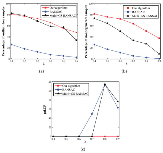
Figure 4.
Performance of sampling methods on the Table dataset as the ratio increases: (a) percentage of outlier-free sample sets, (b) percentage of non-degenerate sample sets and (c) estimation accuracy.
The proposed algorithm drew up to 75-times more outlier-free sample sets in comparison with RANSAC within a limited budget of 1000 sample sets (Figure 4a). The percentages of outlier-free samples for our algorithm and Multi-GS-RANSAC were very close. This showed that the Multi-GS sampling strategy performed well in the absence of degeneracy. However, Multi-GS sampling failed to draw non-degenerate sample sets as the ratio increased (Figure 4b). For ratios higher than , both RANSAC and Multi-GS-RANSAC failed to estimate the model correctly (Figure 4c), while the proposed algorithm estimated the model robustly even in the presence of serious degeneracy ().
5.2.2. Performance under Varying Outlier Ratios
A similar test was performed to assess the performance of the sampling algorithm under various ratios of outliers. To this end, the Church dataset was used. The limited sampling budget was set to 1000 and 5000 sample sets for outlier rates less than or equal to 50% and higher than 50%, respectively. The percentage of outlier-free sample sets among the budgeted sample sets (either 1000 or 5000) and the estimation accuracy () are presented in Figure 5.
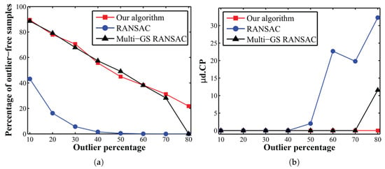
Figure 5.
Performance of sampling methods on the Church dataset as the outlier ratio increases: (a) percentage of outlier-free sample sets, (b) estimation accuracy.
For most of the outlier ratios, the outlier-free sampling rates of the proposed algorithm and those of Multi-GS were very close. RANSAC drew quite less outlier-free sample sets in comparison with the other two methods. For outlier ratios higher than 50%, RANSAC completely failed to detect outlier-free sample sets and to estimate the model correctly. For an outlier ratio of 80%, only the proposed algorithm kept good performance by drawing at least 22% outlier-free sample sets, given the limited sampling budget. As a conclusion, the sampling strategy based on the spatial distribution of correspondences along with the evolutionary search not only increased the speed of reaching an outlier-free sample set, but also decreased the probability of ending up with a degenerate solution.
5.3. Performance of Inlier Classification with Adaptive Thresholding
In order to verify the performance of the proposed thresholding method for inlier classification (Section 4.4), a stereo pair from the Multiview dataset at the baseline of 20 m was used. To eliminate the effect of other components of the algorithm, such as sampling and the objective function, no outlier was introduced to the images; i.e., the dataset was outlier-free. The results from our method were compared with those of the median-based and covariance-based algorithms. To this end, each algorithm was applied 500 times. In any trial, a minimal sample set of eight points was randomly drawn, and the fundamental matrix was estimated with the normalized eight-point algorithm. For our algorithm, the technique of Section 4.4 was applied to determine the inlier thresholds. For the median-based algorithm, the robust standard deviation of residuals was defined as . Since the dataset was outlier-free, n was equal to the total number of matches, and was the residual of any correspondence with respect to the estimated fundamental matrix. Then, the inlier threshold was calculated as . For the covariance-based algorithm, which is the core component of Cov-RANSAC, first, the uncertainty of the estimated model was used to narrow down the total set of matches to the set of potential inliers. Then, the median-based algorithm was applied to the potential inliers for determining the inlier threshold.
In order to evaluate the performance of these algorithms, the fraction of runs (from a total of 500 runs) in which a correspondence was classified as inlier was calculated, namely the inlier probability of that match. The inlier probabilities (sorted in ascending order) are shown in Figure 6. Knowing that the dataset was outlier-free, the inlier probability for all of the points was ideally one. Our thresholding algorithm resulted in the most stable and robust solutions. That is, for 92% of the points, the inlier probability was higher than . For the median-based algorithm, this percentage was only 15%. The covariance-based algorithm had poor performance in comparison with both of the other methods. Our algorithm resulted in inlier ratios higher than 90% for more than 88% of the runs. However, the median-based and covariance-based algorithms yielded inlier ratios greater than 90% at only 32% and 15% of the runs, respectively.
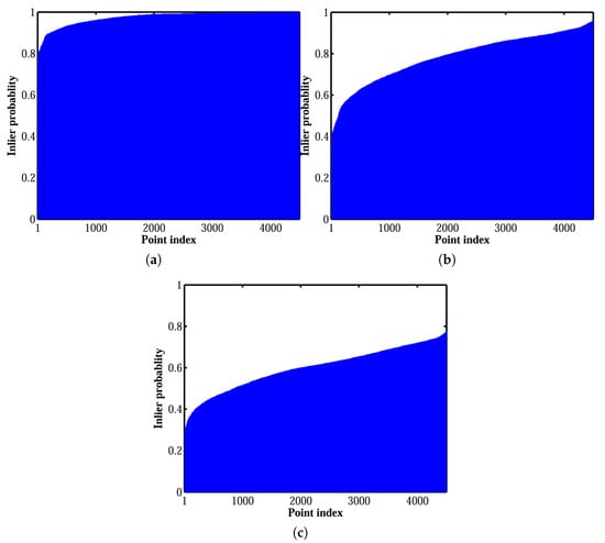
Figure 6.
Inlier probability of correspondences obtained using (a) our adaptive thresholding method: (b) median-based algorithm; (c) covariance-based algorithm.
To investigate the reason behind the performance of each algorithm, the threshold values determined at each run are illustrated versus the run index as black points in Figure 7. Then, the true residuals, which are residuals of the matches from the true fundamental matrix, were calculated. Note that the true fundamental matrix is the one based on which the matches are synthesized. The maximum and the median of the true residuals are shown in Figure 7 as the red and green lines, respectively. Then, the parameter using true residuals was used to calculate the true median-based threshold. The blue line illustrates this value in Figure 7.
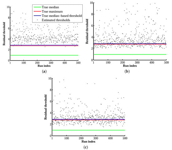
Figure 7.
Inlier thresholds determined by (a) our adaptive thresholding method; (b) the median-based algorithm and (c) the covariance-based algorithm.
The true median-based threshold was slightly higher than the true maximum residual, and it would be an ideal choice of threshold only if the fundamental matrix were perfect. However, in these tests, the fundamental matrix was calculated from a minimal sample set of eight correspondences, which had different values of noise and did not necessarily have an ideal spatial configuration either. Because of the uncertainty of the fundamental matrix and the noise value of the points participating in the estimation of the fundamental matrix, the threshold value should be larger than the ideal one to detect all of the inliers correctly. Although the covariance-based method tried to consider this effect, it underestimated the potential inliers. The main reason was that the uncertainty of the fundamental matrix was estimated only from the minimal sample set. As shown in Figure 7, our algorithm calculated the threshold adaptively. Frequently, the estimated threshold value was slightly higher than the ideal median-based threshold. This was reasonable since the calculated fundamental matrix, although determined from an outlier-free sample set, was not necessarily perfect. However, for the other two methods, the threshold values were approximately around the true median-based threshold, which could be suitable threshold values only if the estimated fundamental matrices were as accurate as the true one.
5.4. Performance under Various Outlier Ratios
To assess the performance of the overall algorithm under different ratios of outliers, the Multiview dataset was used. In the following experiments, the stall generation of the GA was set to 60. The upper bound to the standard deviation of image noise () was set to three pixels. The GA population size was set to 27. The parameter was set to in all of our experiments. The algorithm was implemented in the MATLAB environment directly without using its optimization toolbox. The average of the results over all of the stereo pairs versus the outlier ratios are presented in Figure 8.
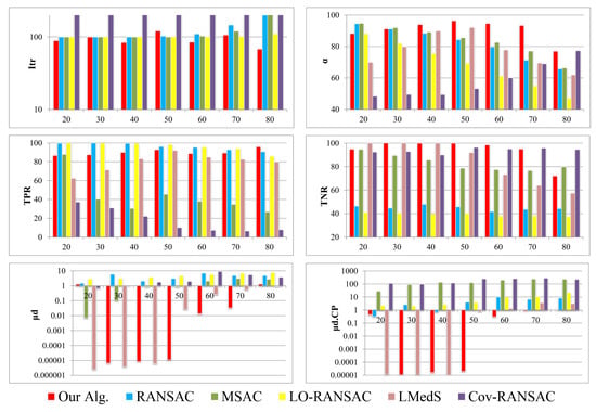
Figure 8.
Performance of different algorithms under various percentages of outliers for the Multiview dataset. In the graphs, the x-axis represents the percentage of synthetic outliers in the dataset.
The results can clearly illustrate the performance of the proposed algorithm. For instance, to reach 95% accuracy in inlier detection from a dataset with 70% outliers, at least 45,658 sample sets must be drawn in random sample consensus. However, the proposed algorithm reached 95% accuracy by drawing only 2100 sample sets. Similarly, our algorithm achieved 78% accuracy over the 80% contaminated dataset with only 1440 hypotheses, while 591,455 random sample sets would be theoretically required to reach that accuracy. There was a combination of reasons caused by the evolutionary search and the sampling strategy that boosted this improvement. Furthermore, for all of the outlier ratios, the number of GA iterations was lower than other algorithms (average Itr of 93). However, it should be noted that any iteration of GA corresponds to the maximum of 27 hypothesis generation. In the case of data with a low percentage of outliers, there are many correct solutions that each can be slightly fitter; such slightly fitter solutions may violate the termination criterion mentioned in Section 4.3. Therefore, an additional condition based on the rate of improvement achieved by the new elites must be considered to avoid unnecessary iterations. One can use the following method; whenever the elite solutions of two generations have fitness values within 10% of one another, then the fitter solution should duplicate itself, and the less fit solution should be removed to ensure a low standard deviation over the stall generations.
From the accuracy point of view, the proposed algorithm was more robust to outliers in comparison with other algorithms, especially when the outlier percentage grew over 40%. On average, the proposed technique achieved 91% ± 6% accuracy for inlier detection. The considerably high estimation accuracy (average of ) confirmed this, as well. The improvement obtained by the proposed algorithm was also evident regarding the true negative rate (average TNR of 94%), which showed the efficiency of the algorithm to distinguish outliers from inliers. Figure 8 also indicates that LMedS performs robustly for outlier ratios less than 50%. However, model estimation and, particularly, inlier detection for higher outlier rates is the bottleneck of this algorithm. The Cov-RANSAC resulted in better TNR compared to our algorithm. However, the spatial configuration and the level of noise in the sampled points are ignored in this method. As a result, the estimation of model uncertainty becomes impractically too large or too small. Consequently, the number of inliers is usually over- or under-estimated. That is why this technique resulted in very low TPR. .
5.5. Performance Stability
Another variable that should be tested under various outlier ratios is the stability of the results obtained by running the algorithm multiple times. To this end, the Church dataset was used. The algorithm was repeated 50 times for each instance of the data. For outlier ratios ranging from 10 to 70%, the variations of accuracy was not considerable ( = 99% 2%). However, at an 80% outlier rate, the average accuracy decreased to 92% ± 8%. Although this was a noticeable change in the performance of the algorithm, the median of the accuracies was yet reasonably high (95%). Regarding the number of models hypothesized before termination, a large range of changes was observed at lower outlier ratios. As explained earlier, this happened due to the stopping criterion in GA. However, this was itself an advantage for large outlier ratios (more than 50% outliers).
5.6. Performance under Various Noise Levels
The Urban dataset was used to evaluate the robustness of the proposed algorithm against noisy image observations. To this end, the effects of image noise along with varying percentages of outliers were tested using 81 instances of the Urban dataset. The results are illustrated in Figure 9.
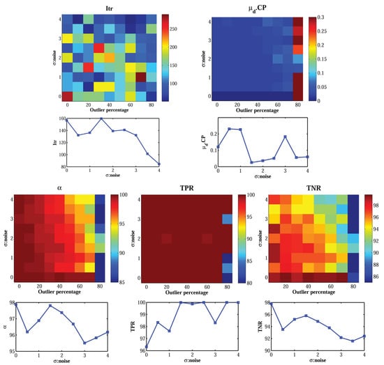
Figure 9.
Performance of the proposed algorithm with noisy images. The graph at the bottom of each surface-plot represents the average of respective performance criterion versus the amount of noise.
From the accuracy point of view, the accuracy of estimation (described by ) did not decrease by increasing the noise level. The different noise synthesized on putative matches varies between zero and four pixels. The robustness of the algorithm to noise means that the sample sets whose points have a lower level of noise can be recognized through the LTS-based objective function. Thus, the estimation of the fundamental matrix would be based on the least-noisy correspondences of the dataset. Regarding the accuracy of inlier detection, the true positive rate was not affected by the noise. However, the true negative rate decreased slightly by increasing the noise level. Since the outliers were synthesized by adding gross errors as low as 10 pixels to correspondences, distinguishing real outliers from noisy inliers at higher noise levels became a more difficult task, and the false positive rate increased. In terms of convergence speed, increasing the magnitude of image noise decreased the number of iterations. The total number of iterations required to find the final solution changed only from 80 to 250 as the ratio of outliers increased to 80% and the level of noise increased to four pixels. This shows the high computational efficiency of the overall algorithm in the presence of high ratios of outliers and noise.
5.7. Effect of the GA Population Size
To evaluate the effect of GA population size on the performance of the algorithm, the Church dataset was applied. The GA population size was varied from 20 to 70 by steps of five individuals, and the performance of the algorithm was assessed under various outlier ratios. The results obtained from this experiment are illustrated in Figure 10.
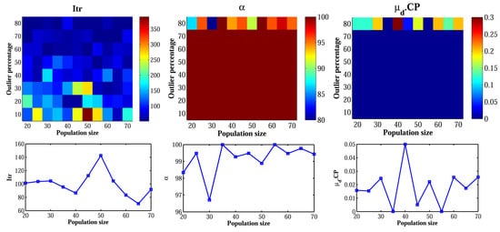
Figure 10.
Performance of the proposed algorithm with varying GA population size. The graph at the bottom of each surface-plot represents the average of the respective performance criterion versus the population size.
There was no considerable correlation between the accuracy and the size of the population. The average accuracy of inlier-detection () with different population sizes was % with a standard deviation of only %. The accuracy of estimation () also remained below , which confirmed the stable accuracy of model estimation. The number of iterations before termination (Itr) seemed to be more dependent on the outlier percentage rather than the population size. The average number of iterations at outlier ratios less than 50% was 122, while it was only 62 at higher outlier ratios. The number of generated hypotheses () increased by either decreasing the outlier ratio or increasing the GA population size, since it depended both on the population size and the number of iterations. Showing that the accuracy does not have any distinct correlation with the population size, the moderate size of the population is suggested to both avoid the unnecessary generation of hypotheses and to keep the number of iterations small.
5.8. Experiments on Real Data
The proposed algorithm of robust estimation and inlier detection was compared with other RANSAC-like techniques for 15 stereo pairs (Table 3). These examples were chosen to cover various cases, such as close-range and aerial photography, narrow and wide baselines, degenerate configurations, scale variation, multi-platform photography and highly contaminated data. The first seven pairs and their putative matches were gathered from [40]. For these data, the percentages of true inliers in the dataset () were manually determined in the reference article. For the 8th, the 9th and the 10th stereo pairs, we used signalized targets to provide ground control data when acquiring the images. The reference fundamental matrices were calculated from these control points. The 11th stereo pair belongs to the ISPRS datasets for urban classification www2.isprs.org/commissions/comm3/wg4/detection-and-reconstruction.html. The 14th stereo pair belongs to the ISPRS benchmark for multi-platform photogrammetry http://www2.isprs.org/commissions/comm1/icwg15b/benchmark_main.html [55]. For these last two pairs, the exterior and interior orientation parameters provided by ISPRS were used as reference values for evaluation. For the last five stereo pairs, SIFT key points were detected and matched using the VlFeat www.vlfeat.org feature-based matching library. For the second and the 12th stereo pairs, we could not apply Multi-GS, since the low inlier ratio and a high number of correspondences made that algorithm too slow to be executable.

Table 3.
Performance of the proposed algorithm and other techniques on real data.
It can be noticed from the results that our algorithm generally yielded solutions that were compatible with the ground-truth in terms of either inlier-detection accuracy or estimation accuracy. For the eight and the ninth images, a dominant plane existed in the scene. Therefore, most of the algorithms ended up with a degenerate solution. However, the degeneracy could be avoided quite efficiently by our algorithm. This was mainly due to the guided sampling based on the spatial distribution of matches. Finally, it was noticed that the algorithm had good performance in challenging cases such as multi-platform photography.
6. Conclusions
In this study, we proposed an integer-coded genetic algorithm for the problem of accurate epipolar-geometry estimation from putative matches, followed by an adaptive thresholding algorithm for inlier classification. The proposed algorithm can be considered as a solution to resolve some of the drawbacks involved in conventional robust estimators, specifically RANSAC-like methods. Based on the experiments, the proposed approach showed robustness to high percentages of outliers, planar degeneracy and image noise. On a general note, the success of the proposed algorithm is due to a combination of elements: (i) the evolutionary behaviour of the search for outlier-free sample sets; (ii) the definition of the objective function to not depend on the maximum number of the inliers, but their minimum number; (iii) the integration of guided sampling and (iv) the uncertainty analysis in the final inlier classification scheme. It should be noted that, except for the first element, other ones could be easily integrated with different iterative robust estimation algorithms, as well. In the future, the proposed sampling and classification techniques will be integrated with the variants of RANSAC, and their improvement will be assessed. In general, the algorithm was able to detect the inliers by more than 85% accuracy, which is a remarkable success for large datasets containing over 80% outliers. Furthermore, the computational expenses of the algorithm were not increasing with either the ratio of outliers or the magnitude of image noise. The efficiency of the proposed algorithm regarding speed was greater than other methods for datasets with a high ratio of outliers (with more than 50% outliers). In the future, the algorithm could also become more robust to degeneracy by extending the proposed two-dimensional guided sampling to three dimensions by finding the probable three-dimensional structures.
Acknowledgments
The authors gratefully acknowledge the substantive contributions of Wolfgang Förstner from Bonn University in reviewing and editing this manuscript and providing the authors with constructive comments. This study is supported in part by grants from the: Centre de Géomatique du Québec (www.cgq.qc.ca), Fonds de Recherche Québécois sur la Nature et les Technologies (www.frqnt.gouv.qc.ca) and Natural Sciences and Engineering Research Council of Canada (www.nserc-crsng.gc.ca). The authors would also like to acknowledge the provision of the datasets (the 12th pair in Table 3) by ISPRS and EuroSDR, released in conjunction with the ISPRS scientific initiative 2014 and 2015, led by ISPRS ICWGI/Vb, as well as the provision of the Downtown Toronto datasets (the 3D point cloud used to simulate the Urban dataset in Table 3 and the 11th pair in Table 3) by Optech Inc., First Base Solutions Inc., GeoICTLab at York University and ISPRS WGIII/4.
Author Contributions
Mozhdeh Shahbazi performed the theoretical developments. Unless otherwise mentioned in the paper, she programmed the software packages for performing the experiments and analysing the results. Furthermore, she prepared the first draft of this manuscript. The manuscript was revised and modified by the other authors. All of the authors assisted in planning the experiments and analysing the results. Gunho Sohn and Jérôme Théau provided the direction and supervision of this study. They provided their constructive comments and consults to perform this study.
Conflicts of Interest
The authors declare no conflict of interest.
References
- Schmidt, A. The EKF-based visual SLAM system with relative map orientation measurements. In Proceedings of the International Conference on Computer Vision and Graphics, Warsaw, Poland, 15–17 September 2014; Springer: Cham, Switzerland, 2014; pp. 570–577. [Google Scholar]
- Hartmann, J.; Klüssendorff, J.H.; Maehle, E. A comparison of feature descriptors for visual SLAM. In Proceedings of the 2013 IEEE European Conference on Mobile Robots (ECMR), Barcelona, Spain, 25–27 September 2013; pp. 56–61. [Google Scholar]
- Wendel, A.; Maurer, M.; Graber, G.; Pock, T.; Bischof, H. Dense reconstruction on-the-fly. In Proceedings of the 2012 IEEE Conference on Computer Vision and Pattern Recognition (CVPR), Providence, RI, USA, 16–21 June 2012; pp. 1450–1457. [Google Scholar]
- Kekec, T.; Yildirim, A.; Unel, M. A new approach to real-time mosaicking of aerial images. Rob. Auton. Syst. 2014, 62, 1755–1767. [Google Scholar] [CrossRef]
- Ghosh, D.; Kaabouch, N. A survey on image mosaicking techniques. J. Vis. Commun. Image Represent. 2016, 34, 1–11. [Google Scholar] [CrossRef]
- He, H.; Du, J.; Chen, X.; Wang, Y. Oblique low-altitude image matching using robust perspective invariant features. In Proceedings of the Seventh International Conference on Electronics and Information Engineering, Nanjing, China, 17 September 2016; p. 103221S. [Google Scholar]
- Li, J.; Allinson, N.M. A comprehensive review of current local features for computer vision. Neurocomputing 2008, 71, 1771–1787. [Google Scholar] [CrossRef]
- Apollonio, F.; Ballabeni, A.; Gaiani, M.; Remondino, F. Evaluation of feature-based methods for automated network orientation. Int. Arch. Photogramm. Remote Sens. Spat. Inf. Sci. 2014, 40, 47. [Google Scholar] [CrossRef]
- Lin, W.Y.; Liu, S.; Jiang, N.; Do, M.N.; Tan, P.; Lu, J. RepMatch: Robust Feature Matching and Pose for Reconstructing Modern Cities. In Proceedings of the European Conference on Computer Vision (ECCV 2016), Amsterdam, The Netherlands, 8–16 October 2016; Springer: Cham, Switzerland, 2016; pp. 562–579. [Google Scholar]
- Radhika, V.; Kartikeyan, B.; Krishna, B.G.; Chowdhury, S.; Srivastava, P.K. Robust stereo image matching for spaceborne imagery. IEEE Trans. Geosci. Remote Sens. 2007, 45, 2993–3000. [Google Scholar] [CrossRef]
- Wang, Y.; Huang, J.; Liu, J.; Tang, X. An efficient image-registration method based on probability density and global parallax. AEU-Int. J. Electron. Commun. 2010, 64, 1148–1156. [Google Scholar] [CrossRef]
- Hasler, D.; Sbaiz, L.; Susstrunk, S.; Vetterli, M. Outlier modeling in image matching. IEEE Trans. Pattern Anal. Mach. Intell. 2003, 25, 301–315. [Google Scholar] [CrossRef]
- Adam, A.; Rivlin, E.; Shimshoni, I. ROR: Rejection of outliers by rotations. IEEE Trans. Pattern Anal. Mach. Intell. 2001, 23, 78–84. [Google Scholar]
- Liu, Z.; An, J.; Jing, Y. A simple and robust feature point matching algorithm based on restricted spatial order constraints for aerial image registration. IEEE Trans. Geosci. Remote Sens. 2012, 50, 514–527. [Google Scholar] [CrossRef]
- Fischler, M.A.; Bolles, R.C. Random Sample Consensus: A Paradigm for Model Fitting with Applications to Image Analysis and Automated Cartography. Commun. ACM 1981, 24, 381–395. [Google Scholar] [CrossRef]
- Torr, P.; Zisserman, A. Robust computation and parametrization of multiple view relations. In Proceedings of the Sixth International Conference on Computer Vision, Bombay, India, 7 January 1998; pp. 727–732. [Google Scholar]
- Torr, P.H.; Zisserman, A. MLESAC: A new robust estimator with application to estimating image geometry. Comput. Vis. Image Underst. 2000, 78, 138–156. [Google Scholar] [CrossRef]
- Torr, P.H.S. Bayesian model estimation and selection for epipolar geometry and generic manifold fitting. Int. J. Comput. Vis. 2002, 50, 35–61. [Google Scholar] [CrossRef]
- Torr, P.H.; Murray, D.W. The development and comparison of robust methods for estimating the fundamental matrix. Int. J. Comput. Vis. 1997, 24, 271–300. [Google Scholar] [CrossRef]
- Bab-Hadiashar, A.; Suter, D. Robust segmentation of visual data using ranked unbiased scale estimate. Robotica 1999, 17, 649–660. [Google Scholar] [CrossRef]
- Choi, J.; Medioni, G. Starsac: Stable random sample consensus for parameter estimation. In Proceedings of the IEEE Conference on Computer Vision and Pattern Recognition (CVPR 2009), Miami, FL, USA, 20–25 June 2009; pp. 675–682. [Google Scholar]
- Raguram, R.; Frahm, J.M.; Pollefeys, M. Exploiting uncertainty in random sample consensus. In Proceedings of the 2009 IEEE 12th International Conference on Computer Vision, Kyoto, Japan, 29 September–2 October 2009; pp. 2074–2081. [Google Scholar]
- Sattler, T.; Leibe, B.; Kobbelt, L. SCRAMSAC: Improving RANSAC’s efficiency with a spatial consistency filter. In Proceedings of the 2009 IEEE 12th International Conference on Computer Vision, Kyoto, Japan, 29 September–2 October 2009; pp. 2090–2097. [Google Scholar]
- Chum, O.; Matas, J. Matching with PROSAC-progressive sample consensus. In Proceedings of the 2005 IEEE Computer Society Conference on Computer Vision and Pattern Recognition (CVPR’05), San Diego, CA, USA, 20–25 June 2005; Volume 1, pp. 220–226. [Google Scholar]
- Lai, T.; Wang, H.; Yan, Y.; Xiao, G.; Suter, D. Efficient guided hypothesis generation for multi-structure epipolar geometry estimation. Comput. Vis. Image Underst. 2017, 154, 152–165. [Google Scholar] [CrossRef]
- Ni, K.; Jin, H.; Dellaert, F. GroupSAC: Efficient consensus in the presence of groupings. In Proceedings of the 2009 IEEE 12th International Conference on Computer Vision, Kyoto, Japan, 29 September–2 October 2009; pp. 2193–2200. [Google Scholar]
- Chin, T.J.; Yu, J.; Suter, D. Accelerated hypothesis generation for multistructure data via preference analysis. IEEE Trans. Pattern Anal. Mach. Intell. 2012, 34, 625–638. [Google Scholar] [CrossRef] [PubMed]
- Cheng, C.M.; Lai, S.H. A consensus sampling technique for fast and robust model fitting. Pattern Recognit. 2009, 42, 1318–1329. [Google Scholar] [CrossRef]
- Hu, M.; McMenemy, K.; Ferguson, S.; Dodds, G.; Yuan, B. Epipolar geometry estimation based on evolutionary agents. Pattern Recognit. 2008, 41, 575–591. [Google Scholar] [CrossRef]
- Chai, J.; De Ma, S. Robust epipolar geometry estimation using genetic algorithm. Pattern Recognit. Lett. 1998, 19, 829–838. [Google Scholar] [CrossRef]
- Rodehorst, V.; Hellwich, O. Genetic algorithm sample consensus (gasac)-a parallel strategy for robust parameter estimation. In Proceedings of the 2006 Conference on Computer Vision and Pattern Recognition Workshop (CVPRW’06), New York, NY, USA, 17–22 June 2006; p. 103. [Google Scholar]
- Matas, J.; Chum, O. Randomized RANSAC with Td,d test. Image Vis. Comput. 2004, 22, 837–842. [Google Scholar] [CrossRef]
- Capel, D.P. An Effective Bail-out Test for RANSAC Consensus Scoring. In Proceedings of the BMVC 2005, Oxford, UK, 5–8 September 2005. [Google Scholar]
- Matas, J.; Chum, O. Randomized RANSAC with sequential probability ratio test. In Proceedings of the Tenth IEEE International Conference on Computer Vision (ICCV’05), Beijing, China, 17–21 October 2005; Volume 2, pp. 1727–1732. [Google Scholar]
- Chum, O.; Matas, J. Optimal randomized RANSAC. IEEE Trans. Pattern Anal. Mach. Intell. 2008, 30, 1472–1482. [Google Scholar] [CrossRef] [PubMed]
- Nistér, D. Preemptive RANSAC for live structure and motion estimation. Mach. Vis. Appl. 2005, 16, 321–329. [Google Scholar] [CrossRef]
- Chum, O.; Werner, T.; Matas, J. Two-view geometry estimation unaffected by a dominant plane. In Proceedings of the 2005 IEEE Computer Society Conference on Computer Vision and Pattern Recognition (CVPR’05), San Diego, CA, USA, 20–25 June 2005; Volume 1, pp. 772–779. [Google Scholar]
- Lebeda, K.; Matas, J.; Chum, O. Fixing the locally optimized ransac–full experimental evaluation. In Proceedings of the British Machine Vision Conference, Guildford, UK, 3–7 September 2012; pp. 1–11. [Google Scholar]
- Frahm, J.M.; Pollefeys, M. RANSAC for (Quasi-)Degenerate data (QDEGSAC). In Proceedings of the IEEE Computer Society Conference Computer Vision and Pattern Recognition (CVPR’06), New York, NY, USA, 17–22 June 2006; Volume 1, pp. 453–460. [Google Scholar]
- Raguram, R.; Chum, O.; Pollefeys, M.; Matas, J.; Frahm, J.M. USAC: A universal framework for random sample consensus. IEEE Trans. Pattern Anal. Mach. Intell. 2013, 35, 2022–2038. [Google Scholar] [CrossRef] [PubMed]
- Armangué, X.; Salvi, J. Overall view regarding fundamental matrix estimation. Image Vis. Comput. 2003, 21, 205–220. [Google Scholar] [CrossRef]
- Hartley, R.; Zisserman, A. Multiple View Geometry in Computer Vision; Cambridge University Press: Cambridge, UK, 2003. [Google Scholar]
- Hartley, R.I. In defense of the eight-point algorithm. IEEE Trans. Pattern Anal. Mach. Intell. 1997, 19, 580–593. [Google Scholar] [CrossRef]
- Zhong, H.; Pang, Y.; Feng, Y. A new approach to estimating fundamental matrix. Image Vis. Comput. 2006, 24, 56–60. [Google Scholar] [CrossRef]
- Golub, G.H.; Van Loan, C.F. Matrix Computations; JHU Press: Baltimore, MD, USA, 2012; Volume 3. [Google Scholar]
- Zhang, Z. Determining the epipolar geometry and its uncertainty: A review. Int. J. Comput. Vis. 1998, 27, 161–195. [Google Scholar] [CrossRef]
- Zheng, Y.; Sugimoto, S.; Okutomi, M. A practical rank-constrained eight-point algorithm for fundamental matrix estimation. In Proceedings of the IEEE Conference on Computer Vision and Pattern Recognition, Portland, OR, USA, 23–28 June 2013; pp. 1546–1553. [Google Scholar]
- Chesi, G.; Garulli, A.; Vicino, A.; Cipolla, R. Estimating the fundamental matrix via constrained least-squares: A convex approach. IEEE Trans. Pattern Anal. Mach. Intell. 2002, 24, 397–401. [Google Scholar] [CrossRef]
- Hubert, M.; Rousseeuw, P.J.; Van Aelst, S. High-breakdown robust multivariate methods. Stat. Sci. 2008, 23, 92–119. [Google Scholar] [CrossRef]
- Deep, K.; Singh, K.P.; Kansal, M.; Mohan, C. A real coded genetic algorithm for solving integer and mixed integer optimization problems. Appl. Math. Comput. 2009, 212, 505–518. [Google Scholar] [CrossRef]
- Chum, O.; Matas, J.; Kittler, J. Locally optimized RANSAC. In Joint Pattern Recognition Symposium; Springer: Berlin/Heidelberg, Germany, 2003; pp. 236–243. [Google Scholar]
- Engelbrecht, A.P. Computational Intelligence: An Introduction; John Wiley & Sons: Chichester, UK, 2007. [Google Scholar]
- Myatt, D.R.; Torr, P.; Nasuto, S.J.; Bishop, J.M.; Craddock, R. NAPSAC: High noise, high dimensional robust estimation. In Proceedings of the British Machine Vision Conference, Cardiff, UK, 2–5 September 2002. [Google Scholar]
- Sur, F.; Noury, N.; Berger, M.O. Computing the uncertainty of the 8 point algorithm for fundamental matrix estimation. In Proceedings of the 19th British Machine Vision Conference (BMVC 2008), London, UK, 7–10 September 2008; p. 10. [Google Scholar]
- Nex, F.; Gerke, M.; Remondino, F.; Przybilla, H.; Baumker, M.; Zurhorst, A. ISPRS Benchmark for multi-platform photogrammetry. ISPRS Ann. Photogramm. Remote Sens. Spat. Inf. Sci. 2015, 2, 135–142. [Google Scholar] [CrossRef]
© 2017 by the author. Licensee MDPI, Basel, Switzerland. This article is an open access article distributed under the terms and conditions of the Creative Commons Attribution (CC BY) license (http://creativecommons.org/licenses/by/4.0/).
