An Improved Brain-Inspired Emotional Learning Algorithm for Fast Classification

Abstract

Classification is an important task of machine intelligence in the field of information. The artificial neural network (ANN) is widely used for classification. However, the traditional ANN shows slow training speed, and it is hard to meet the real-time requirement for large-scale applications. In this paper, an improved brain-inspired emotional learning (BEL) algorithm is proposed for fast classification. The BEL algorithm was put forward to mimic the high speed of the emotional learning mechanism in mammalian brain, which has the superior features of fast learning and low computational complexity. To improve the accuracy of BEL in classification, the genetic algorithm (GA) is adopted for optimally tuning the weights and biases of amygdala and orbitofrontal cortex in the BEL neural network. The combinational algorithm named as GA-BEL has been tested on eight University of California at Irvine (UCI) datasets and two well-known databases (Japanese Female Facial Expression, Cohn–Kanade). The comparisons of experiments indicate that the proposed GA-BEL is more accurate than the original BEL algorithm, and it is much faster than the traditional algorithm.

1. Introduction

Classification has been widely used in the area of machine learning, pattern recognition and data mining. Various artificial intelligence methods, such as the artificial neural network (ANN) [1], support vector machine (SVM) [2], decision tree [3], extreme learning machine [4], the linear regression classifier [5] and other classifiers, have been proposed for classification problems. Among these methods, ANN is very popular due to the features of self-learning, self-adaptive and high generalization capability. However, the traditional ANN has been proven to have some significant drawbacks, such as low training speed, high computational complexity, and the convergence rate makes it hard to meet the requirements of real-time classification [6].

Recently, owing to the neurobiology and cognition research of emotion, emotional intelligence is playing an important role in artificial intelligence [7], and it has attracted an increasing interest around the world. Many bio-inspired brain emotional learning (BEL) models have been proposed and successfully applied in intelligent engineering applications [8,9]. These models are based on the amygdala-orbitofrontal model proposed by Morén et al. [10], which was inspired by the LeDoux’s anatomical findings of the limbic system in mammalian brain [11]. According to the LeDoux’ finding, amygdala and orbitofrontal cortex are two main parts of the limbic system, and they interact to process emotional stimulus correctly and rapidly. Therefore, BEL-based models that mimic the high speed of the emotional learning mechanism in the limbic system have the superior features of fast learning and quickly reacting, and they are widely used in classification [12], prediction [13] and control applications [14].

In the amygdala-orbitofrontal model, the reward signal is important to adjust the weights of amygdala and orbitofrontal cortex in the emotional learning process, but it is not clearly defined so far. Many researchers have proposed different versions of BEL models based on the amygdala-orbitofrontal model, as well as different reward signal determinations. Lucas et al. [15] proposed the BEL-based controller and explicitly determined the reward signal as PID formulization, which has been successfully applied in intelligent engineering applications. Abdi et al. [16] applied a BEL model to prediction short-term traffic flow and defined the reward signal as the multiplication of some related weight. Parsapoor [17] presents a BEL-based architecture for chaotic time series prediction. Although these BEL-based models achieve success in applications, they are based on reinforcement learning to adjust the weights of amygdala and orbitofrontal cortex in the BEL model, and they cannot be generalized to other issues for their characteristic of model sensitive. Lotfi et al. [18] proposed a novel BEL-based pattern recognizer, which employed a pattern-target method instead of the reward-based reinforcement learning to update the weights of amygdala and orbitofrontal cortex. Although this is a model free method, it reduces the precision of the learning process, and the classification accuracy needs to be further improved.

In this study, we aim to propose a more accurate BEL algorithm for fast classification. It has been demonstrated that the neural network classification accuracy can be substantially improved by optimizing the weights of the network [19]. There are many optimization methods, such as genetic algorithm (GA) [20], particle swarm optimization (PSO) [21], differential evolution (DE) [22], and so on. Compared to GA, PSO and DE are relatively simple and easily converge, but they are easily trapped into local minimum in the searching process and show a slight compromise in accuracy. While GA can evolve the population to a better area of the search space and it has good global searching ability [19], the BEL algorithm has the advantage of fast learning, but shows a compromise in accuracy. We aim to optimize the BEL algorithm and make it more accurate. Therefore, we adopted the effective GA to optimize the BEL model. The integrated algorithm named as GA-BEL takes advantage of the fast learning and low computational complexity of BEL, as well as the global optimum solution of GA. Thus, GA-BEL is expected to achieve better performances than the original BEL in classification applications. The GA-BEL is tested on eight University of California at Irvine (UCI) classification datasets, for two facial recognition problem. Results indicated the superiority of the proposed GA-BEL in terms of classification accuracy and execution speed.

The rest of this paper is organized as follows. Section 2 offers the brief related work on BEL. The improved BEL neural network and the implementation of GA-BEL algorithm are described in Section 3. In Section 4, the detailed experimental design is described, as well as the empirical results and discussions. Finally, conclusions and future work are summarized in Section 5.

2. Anatomical Foundation and Related Works

The description of the emotional brain is based on the limbic system theory [11]. Figure 1a [18] shows the limbic system in the emotional brain and its components, including the sensory cortex, thalamus, amygdala, orbitofrontal cortex, etc. There are two main parts among these components. One is amygdale, which plays a critical role in emotional learning and reacting. The other is orbitofrontal cortex, which assists amygdala to process emotional stimulus. LeDoux [23] argues that emotional stimuli can reach the amygdala by two different ways, as shown is Figure 1b. One is short and fast, coming directly from the thalamus, and the other is long and slow, coming from the sensory cortex. Amygdala is properly situated to reach the stimuli extremely quickly and produce the required reaction. Due to the existence of a short path in the emotional brain, emotional stimuli are processed much faster than normal stimuli.

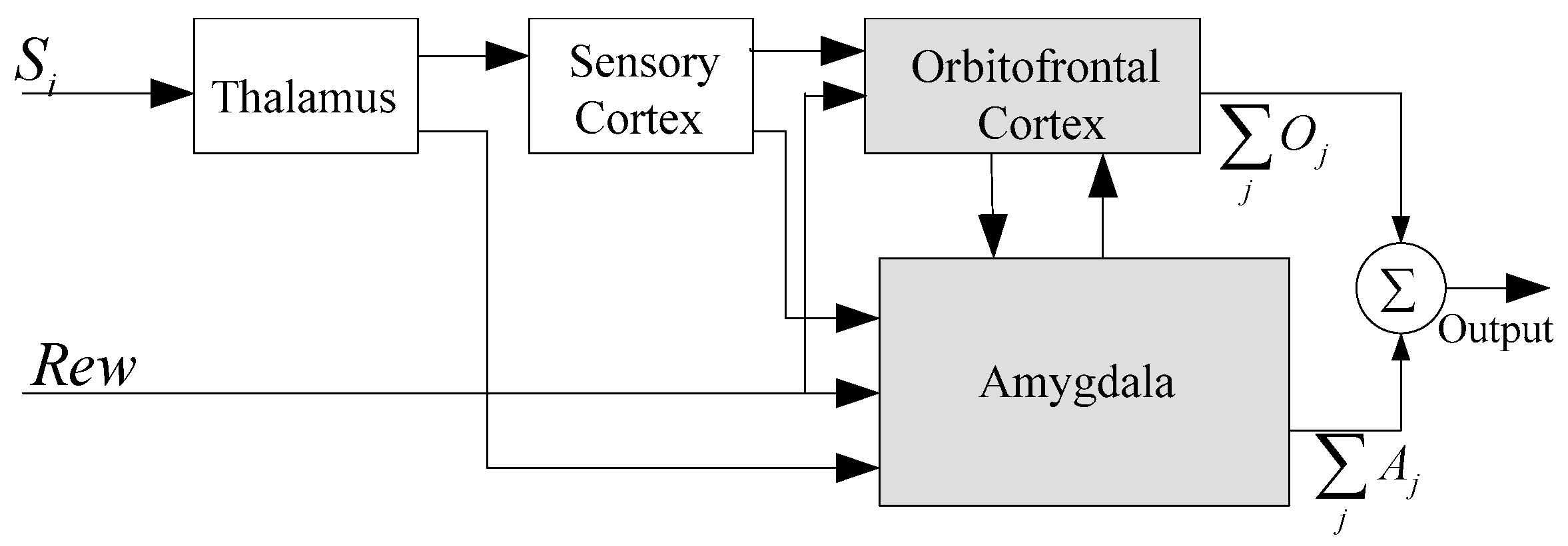
Motivated by LeDoux’s anatomical findings in the emotional brain, Morén et al. [10] proposed the amygdala-orbitofrontal model in 2000, the framework of amygdala-orbitofrontal model is shown in Figure 2. The structure is inherited from some parts of the limbic system (e.g., the amygdala, thalamus, sensory cortex) and imitates the interaction between those parts of the limbic system. In the amygdala-orbitofrontal model, amygdala and orbitofrontal cortex are essential for emotional learning and reacting. Amygdala receives emotional stimuli from the sensory cortex and thalamus, as well as the external reward signal, and it interacts with the orbitofrontal cortex and reacts to the emotional stimuli based on the reward signal. The orbitofrontal cortex receives sensory input from the sensory cortex, as well, and evaluates the amygdala’s response to prevent inappropriate learning connections. They interact frequently to mimic the functionality of the emotional brain responsible for processing emotional stimulus.

In the amygdala-orbitofrontal model, S_i is the sensory input; A_j is the output of the amygdala; O_j is the output of the orbitofrontal cortex. The reward signal Rew is used to update the weights of amygdale and orbitofrontal cortex in emotional learning, and learning rules are expressed as follows [10]:

$$\Delta v_i=\alpha (S_i\max (0,Rew-{\displaystyle \sum _j{A}_j}))$$

(1)

$$\Delta w_i=\beta (S_i{\displaystyle \sum _j(O_j-Rew)})$$

where Δv_i and Δw_i represent the weight of amygdala and orbitofrontal cortex, respectively, and $\alpha$ and $\beta$ are learning rates, which are used to adjust the learning speed. The reward signal Rew is used to adjust the weights of amygdala and orbitofrontal cortex in the emotional learning process.

Various modified BEL models that are based on the amygdala-orbitofrontal model have been proposed, as well as the reward signal determination. In the modified BEL model in [16], the reward signal Rew is defined as follows:

$$Rew={\displaystyle \sum _j{w}_j{r}_j}$$

(2)

where r stands for the factors of the reinforcement agent, and w represents the related weights.

Although these BEL-based models achieve success in the applications, most of them are based on the reinforcement learning to adjust the weights of amygdala and orbitofrontal cortex; they are model sensitive and cannot be generalized to other issues.

Lotfi et al. [18] employed activation functions and the target value (T) of the input pattern to update the weights of amygdala and orbitofrontal cortex in the learning phase, i.e., $Rew=T$. Thus, the supervised learning rules are described as follows:

$$v_j^{k+1}=(1-\gamma )v_j^k+\alpha \max (T^k-E_a^k,0)p_j^k,j=1,2,...,n+1$$

(3)

$$w_j^{k+1}=w_j^k+\beta (E^k-T^k)p_j^k,j=1,2,...,n$$

where $v_j^k$ and $w_j^k$ represent the weight of amygdala and orbitofrontal cortex, respectively, T^k is the target value associated with the k-th pattern pk, $E_a^k$ is the output of amygdala, E^k is the final output, k is a learning step and $\alpha$ and $\beta$ are learning rates. Additionally, $\gamma$ is the decay rate in the amygdala learning rule. The model can be employed to learn the pattern-target relationship of an application by using emotional learning, but this method reduces the precision of the learning process, and the classification accuracy needs to be improved.

3. Implementation

3.1. Improved BEL Neural Network

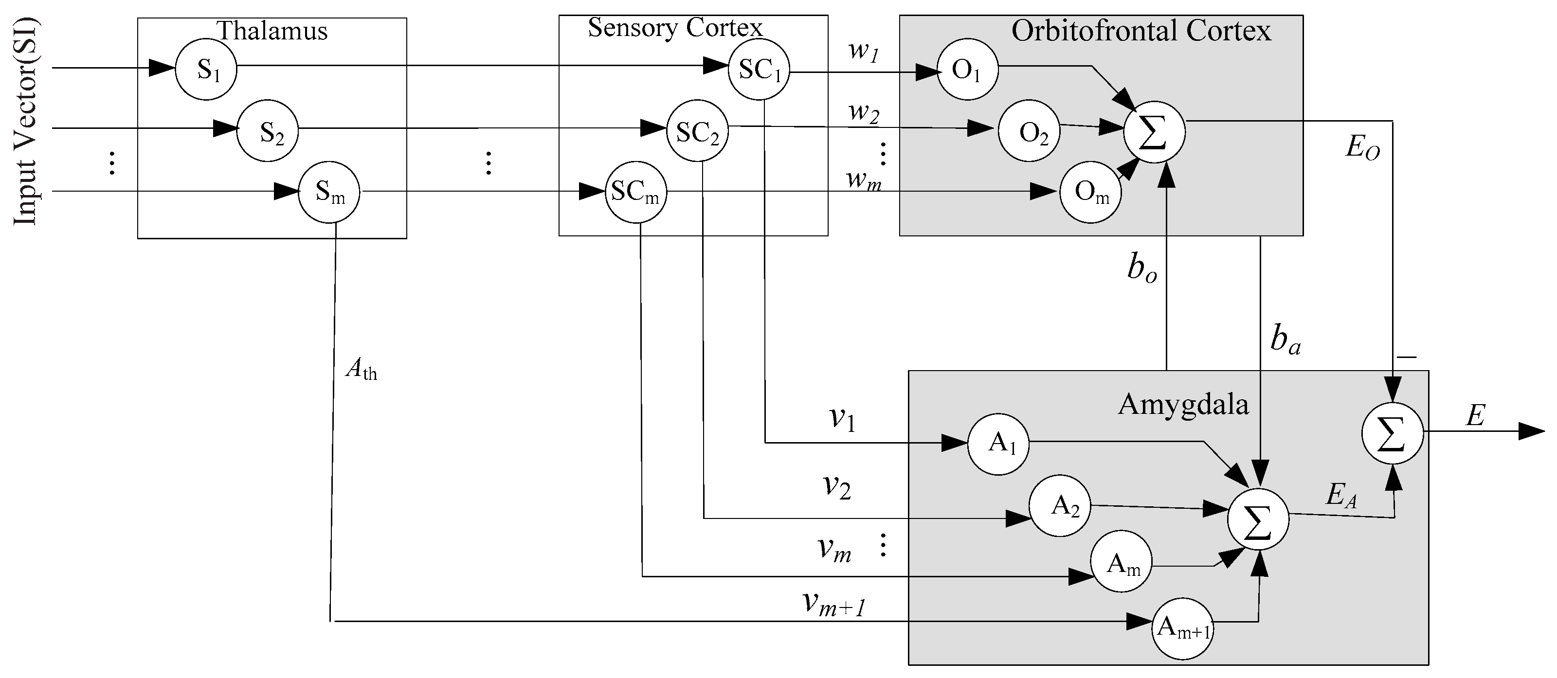
In contrast to previous BEL-based models, we apply the fitness function in GA instead of reinforcement learning to update the weights of amygdale and orbitofrontal cortex in emotional learning. Therefore, we delete the reward signal in the BEL neural network. In addition, according to the biological interaction between amygdale and orbitofrontal cortex in the emotional learning, we add the bias for each part. The improved BEL-based neural network is shown in Figure 3, which consists of four common subsystems including thalamus, sensory cortex, orbitofrontal cortex and amygdala. Amygdala and orbitofrontal cortex are the two main subsystems, which are mainly responsible for emotional learning.

The model is presented as a multiple input-single output architecture; amygdala receives m input vectors SI = [S₁, S₂,…, S_m] from the sensory cortex and A_th from the thalamus; A_th is calculated by Equation (4) [10]:

$$A_{\mathrm{th}}=\max (S_1,S_2,...,S_m)$$

(4)

As shown in Figure 3, v_i is the amygdala weight, and b_a is the bias of amygdala neuron. E_A is the output of the amygdala, and it is calculated by Equation (5) [10]:

$$\begin{array}{l}{A}_i=S_i\cdot v_i,i=1,2,...,m\\ A_{m+1}=A_{th}\cdot v_{m+1}\\ E_A={\displaystyle \sum _{i=1}^{m+1}{A}_i}+b_a={\displaystyle \sum _{i=1}^m{S}_i}\cdot v_i+A_{th}{v}_{m+1}+b_a\end{array}$$

(5)

Furthermore, the orbitofrontal cortex receives the input patterns from the sensory cortex. E_O is the output of the orbitofrontal cortex that is used to inhibit the amygdala’s output, which is calculated by Equation (6) [10]:

$$\begin{array}{l}{O}_i=S_i\cdot w_i,i=1,2,...,m\\ E_O={\displaystyle \sum _{i=1}^m{O}_i}+b_o={\displaystyle \sum _{i=1}^m{S}_i}\cdot w_i+b_o\end{array}$$

(6)

where w_i are orbitofrontal cortex weights and b_o is the bias of orbitofrontal cortex neuron.

Finally, the final output is simply calculated by Equation (7) [10]:

$$E=E_A-E_O$$

(7)

where E is the final output that represents the correct amygdala response.

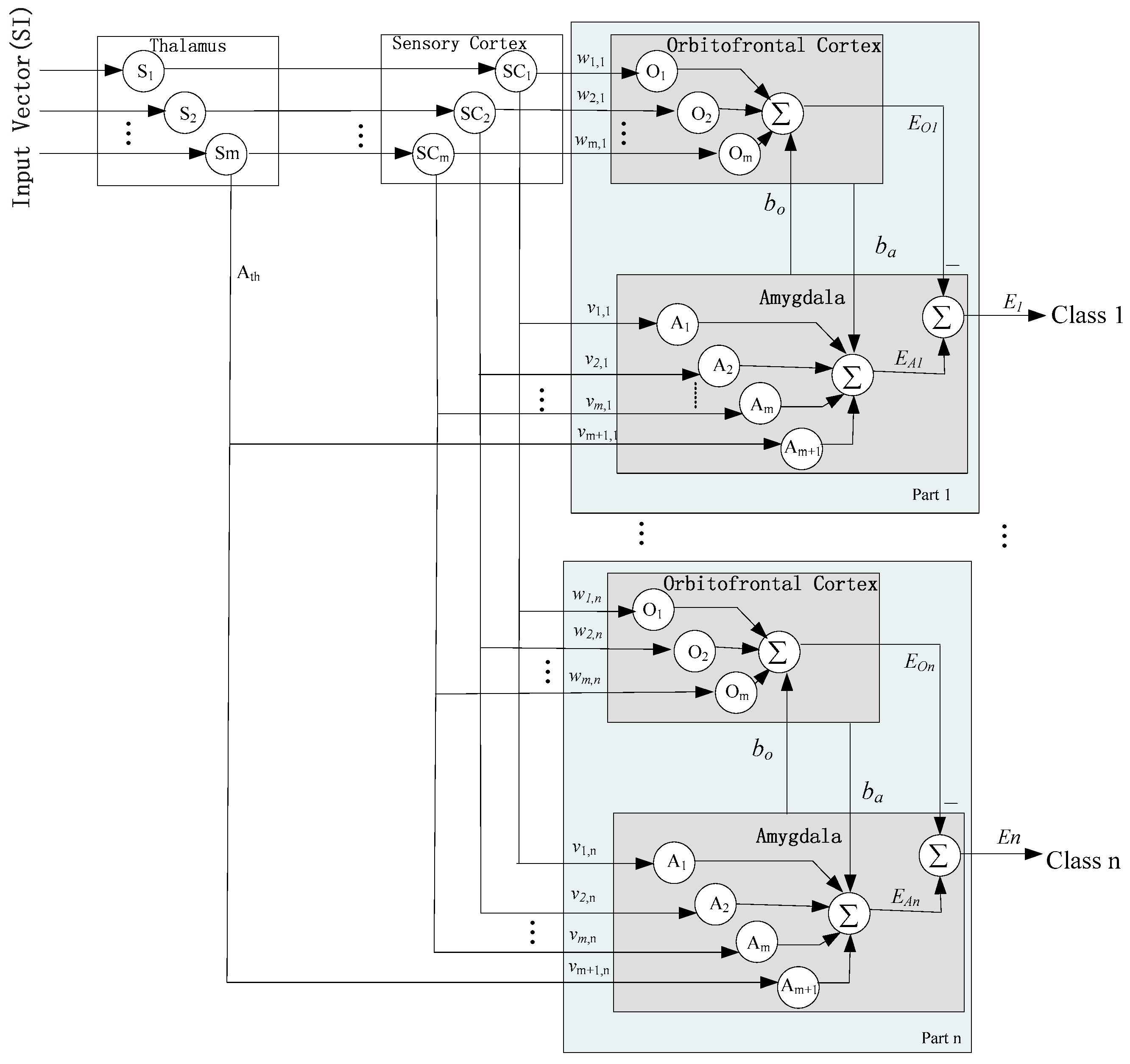
The improved single-output BEL neural network can be learned by pattern-target examples; it is model free and can be utilized in classification application. The number of features in the input vector determines the number of neurons in the thalamus and sensory cortex units, and the number of classes determines the number of orbitofrontal cortex and amygdala units. As a result, the improved BEL model can be extended to generalize in multi-classification applications, and the architecture is shown in Figure 4.

In the proposed m-n BEL network as shown in Figure 4, m is the number of inputs, and n is the number of outputs; there are n amygdala-orbitofrontal cortex parts; in this network, each output unit is associated with one amygdala-orbitofrontal cortex part that interacts separately. Although the distinctive feature of BEL network is fast learning, the network easily is trapped into local minimum. Therefore, the performance of classification accuracy needs to be improved.

3.2. GA-BEL Algorithm

In this paper, GA is adopted to optimize the initial weights and biases of amygdala and orbitofrontal cortex in the BEL neural network. There are three steps in GA-BEL for classification.

● Step 1: Chromosome encoding. For the advantages of high precision, in this paper, real encoding is adopted to acquire optimal results. One real number string presents one chromosome, which consists of the connection weights and bias of orbitofrontal cortex and amygdala. According to the structure of the BEL neural network, each chromosome is initialized as follows:

$$Ch=[w_1,...,w_m,b_o,v_1,...,v_{m+1},b_a]$$

(8)

where w_i and b_o represent orbitofrontal cortex weights and biases, respectively. v_i and b_a represent amygdala weights and bias, respectively. The values of them are usually chosen in [−1, 1]. m is the number of input features; thus, the number of genes in each chromosome is 2m + 3.

● Step 2: Optimization. The value of individual fitness can be calculated by the fitness function. The most optimal fitness value corresponding to the best individual can be found by the selection, crossover and mutation in GA.

(1) Fitness function:

The fitness function is used to evaluate the adaptability of each individual in the whole population, and the individual fitness will provide reference to selection operation. As a consequence, we select the sample variance as the evaluation criteria of weights, and the fitness function is defined as:

$$Fitness(C{h}_k)=\frac{1}{n}\sqrt{{\displaystyle \sum _{k=1}^n{(E_k-T_k)}^2}}$$

(9)

where E_k is the response to the k-th input pattern with given weights in Ch_k, which can be calculated by Equation (7). T_k is the target value; n is the number of pattern-targets. On the definition of the fitness function, the minimum output of the fitness function means the minimum total error for all training samples. Thus, the overall goal of genetic operators is to find the minimum value of the fitness function.

(2) Selection:

The selection operation can choose better individuals for the subsequent iteration. There are several methods of selection in GA, such as the roulette wheel method, the championship method, the optimum maintaining strategy, etc. [24]. In this study, according to the definition of the fitness function, we adopt the roulette wheel method based on the fitness ratio, for the method works by selecting chromosomes with a higher probability of survival, it is intuitive and widely used in GA. According to the definition of the fitness function, the selection probability p_i for each individual i is:

$$\{\begin{array}{l}{f}_i=k/F_i\\ p_i=f_i/{\displaystyle \sum _{j=1}^n{f}_j}\end{array}$$

(10)

where F_i is the fitness value of individual i, k is the coefficient and n is the number of individuals in a group.

(3) Crossover:

To enlarge the diversity and searching space, the crossover operation is used to produce two new individuals by exchanging information between the parent individuals. For crossover mechanisms, single-point crossover, two-point crossover, arithmetic crossover and multipoint crossover are reported [24]. This paper uses a real coded GA strategy in chromosomes. Here, arithmetic crossover is adopted; it is a method with high precision. The rule is given as follows [25]:

$$\{\begin{array}{l}{c}_i^k(n+1)=\alpha c_i^k(n)+(1-\alpha )c_j^k(n)\\ c_j^k(n+1)=\alpha c_j^k(n)+(1-\alpha )c_i^k(n)\end{array}$$

(11)

where $c_i^k$ and $c_j^k$ represent the chromosomes for which occur crossovers in the k-th bit, n denotes the number of iterations and $\alpha$ is a random number uniformly distributed in [0, 1].

(4) Mutation:

To further enhance the local search capability of GA, mutation is another way to create new individuals. The mutation operation is needed to change one or some gene values of the chromosome. For mutation mechanisms, simple mutation, uniform mutation, non-uniform mutation and boundary mutation are reported [24]. Here, we adopt the uniform mutation strategy with a small mutation probability, for it can make a uniform search in the searching space in early generations, and it can also greatly reduce the risk of premature convergence. The mutation operation is defined as [26]:

$$\begin{array}{l}{c}_i^j(g+1)=\{\begin{array}{l}{c}_i^j(g)+(c_i^j(g)-c_{\max })*f(g),r_1>0.5\\ c_i^j(g)+(c_{\min }-c_i^j(g))*f(g),r_1\le 0.5\end{array}\\ f(g)=r_2{(1-g/G_{\max })}^2\end{array}$$

(12)

where $c_i^j$ represents the chromosome for which occurs mutation in the j-th bit, c_max is the upper limit of the allele and c_min is the lower limit, g represents current generation, G_max is the max iteration and r₁ and r₂ are random numbers within the range [0, 1].

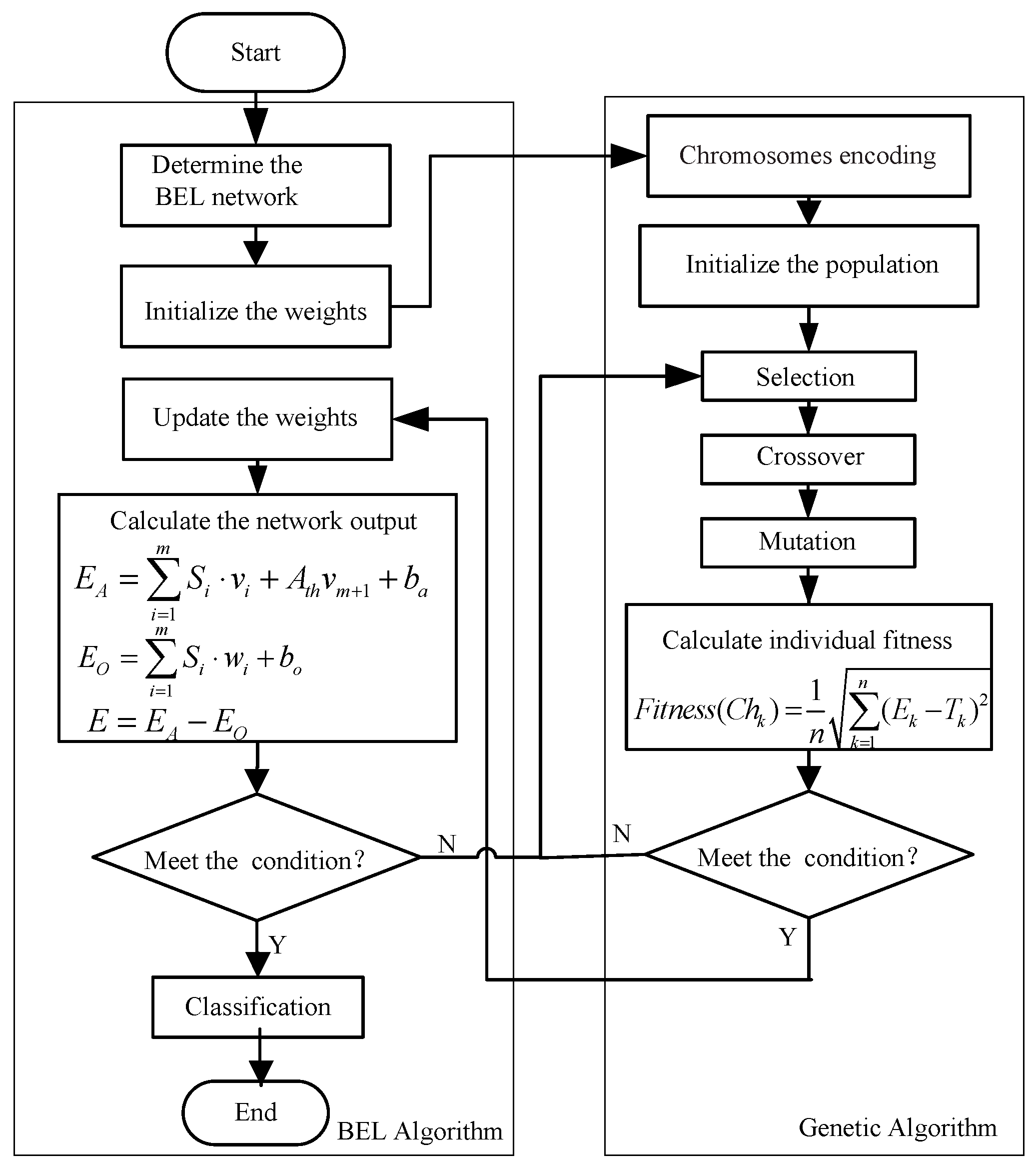
● Step 3: Classification. After the operations of selection, crossover and mutation, the best chromosome can be found that represents the best weights. The original weights and biases are reassigned by the best chromosome, and the trained network is used to classify. The iterative process can be terminated when the result reaches a defined condition. The flowchart of the GA-BEL algorithm is given in Figure 5.

In this paper, the GA-BEL algorithm is implemented by MATLAB. According to the fitness function, the process of optimization is to evaluate the output of the BEL network. Therefore, the main task is the simulation of the BEL network, which can be described as follows:

• /* Matlab code for BEL network simulation */
• function E = sim(net,SI)
• [numSample] = size(SI,2);
• nf = net.numInputs;
• for i = 1:numSample
• E_A = sum(net.amygdalaWeights.* SI(1:nf,i)) + net. AthWeights(1,1) * SI(nf + 1,i) + net. biasA;
• E_O = sum(net.frontalWeights.* SI(1:nf,i)) + net. biasO;
• E(1,i) = E_A - E_O;
• end

4. Simulation Results

In this section, two different experiments are constructed to evaluate the performance of the proposed GA-BEL algorithm. The first experiment is built to show the performance of GA-BEL on the benchmark UCI datasets. The second experiment is arranged to test the GA-BEL on the well-known Japanese Female Facial Expression (JAFFE) and Cohn–Kanade facial expression databases. The comparative experiments are carried out in the two cases. Both experiments are performed in MATLAB R2010b running in an Intel core-i7 3.4 GHz CPU with 8.00 GB RAM and the Windows 7 operation system.

4.1. Case 1: UCI Datasets’ Classification

4.1.1. Datasets’ Description

Eight benchmark datasets are from the University of California at Irvine (UCI) repository [27] of the machine learning database. In this paper, binary and multiclass datasets are both included, which are of relatively high or low dimensions, large or small sizes, and the details are summarized in

Table 1. Datasets’ description.

Attributes	Datasets	#Samples	#Features	#Classes
Low Demensions Small Sizes	Iris	150	4	3
	Breast Cancer	699	9	2
Low Demensions Large Sizes	Banana	5300	2	2
	SVMguide1	7089	4	2
High Demensions Small Sizes	Heart	270	13	2
	Wine	178	13	3
High Demensions Large Sizes	Satimage	6435	36	6
	Segment	2310	19	7

.

4.1.2. Measure for Performance Evaluation

Classification performance can be evaluated by the confusion matrix as described in Figure 6, in which measures such as accuracy, precision and recall are commonly used to assess the performance of bankruptcy classification systems.

where TP is the number of true positives, FN is the number of false negatives, TN is the number of true negatives and FP is the number of false positives. The accuracy, recall and precision are calculated by the following formulas:

$$\begin{array}{l}\mathrm{Accuracy}=\frac{TP+TN}{TP+FP+TN+FN}\times 100\%\\ \mathrm{Recall}=\frac{TP}{TP+FN}\times 100\%\\ \mathrm{Precision}=\frac{TP}{TP+FP}\times 100\%\end{array}$$

(13)

The performance of the execution speed can be evaluated by the computing time in the training and testing process.

4.1.3. Experimental Results and Discussion

4.1.3.1. Classification on Breast Cancer Dataset

The detailed parameter settings in GA-BEL are separate for BEL and GA. For the BEL network, the input patterns determine the number of input neurons, and the classes determines the number of output neurons. Therefore, for the Breast Cancer dataset, the number of the input nodes and output nodes is set to nine and two, respectively. The number of hidden nodes is set to six after many tests. The initialization of the weights and biases is chosen randomly within the range of [−1, 1]. For GA, the value of the population size is based on the chromosome encoding defined in Equation (8), in which the number of genes in each chromosome is 2m + 3; m is the number of features. The Breast Cancer dataset has nine features. Thus, the population size was set to 21 (2 × 9 + 3 = 21). Other parameters’ settings were based on the methods related to artificial neural network optimized by GA [25,26]. Finally, we obtained the best configuration after many tests. Here, the population groups and maximal generation are set to 200 and 100, respectively. The crossover probability and mutation probability are set to 0.8 and 0.03, respectively. Seventy percent of samples are used as training data, and the remaining 30% of samples are used for validation and test purposes. The simulation results are shown in Figure 7.

Figure 7a shows the best and mean fitness corresponding to each generation during the evolution. It can be observed that the fitness curves gradually improved from Generation 1–100 and exhibits no significant improvements after Iteration 90, eventually stopping at Generation 100. This phenomenon demonstrates that GA-BEL comes to convergence and obtains the best chromosome by the evolution.

From the confusion matrix in Figure 7b, we can see that the classification accuracy (Row 3-Column 3) is 96.1% and 97.6% in the training and testing samples, respectively. The precision (Row 1-Column 3) and recall (Row 3-Column 2) of the classification are also given in the two confusion matrices.

As described above, the proposed GA-BEL aims to enhance the BEL classification accuracy by optimizing the parameters of weights and biases in the BEL network. For comparison, we conducted the comparative study between GA-BEL and BEL on the Breast Cancer dataset. Fifty trials have been conducted for each algorithm; the results in terms of precision, recall, accuracy and computing time were recorded. To ensure that the improvements obtained by using the proposed GA-BEL are significant, a statistical validation based on the Kruskal–Wallis (K-W) test [28] was performed. Results including the average precision, recall, accuracy, computing time, as well as the p-value by the K-W test are listed in

Table 2. Experimental results of BEL vs. GA-BEL on the Breast Cancer dataset.

Performance Metric	BEL	GA-BEL	Paired K-W Test p-Value
Precision (%)	97.3	98.5	0.0356
Recall (%)	94.5	95.6	0.0202
Accuracy (%)	94.9	97.5	0.0183
Time (s)	8.27 × 10−3	7.63 × 10−3	0.0316

.

As illustrated in Table 2, the results obtained from GA-BEL outperform BEL. The average accuracy has been improved by 2.6%; the resultant p-value by the K-W test is 0.0183; the value is less than a chosen significance level of 0.05. It can be confirmed that there is statistically significance between the results. The other comparisons in terms of average precision, recall and the computing time are at the statistical significance level of 0.05.

4.1.3.2. Classification on the Heart Dataset

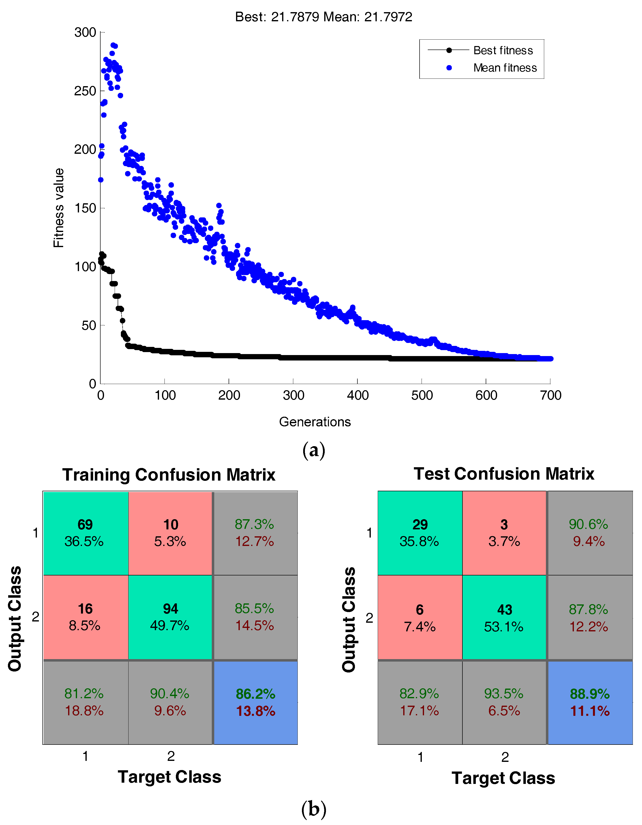
To evaluate the GA-BEL on the relatively small-sized and high dimensional datasets, we chose the Heart dataset for the test. The configuration in the test changed with every dataset. This is because the attributes of the datasets are different. The Heart dataset has 270 samples with 13 features. According to the features of the Heart dataset, the input nodes, hidden nodes and output nodes are respectively set to 13, 6, 2 after many tests. The initialization of the weights and biases is chosen randomly within the range of [−1, 1]. For GA, the population size was set to 29 based on the chromosome encoding defined in Equation (8). The Heart dataset has 13 features. Thus, the population size was set to 29 (2 × 13 + 3 = 29). Other parameters’ settings were based on the methods related to artificial neural network optimized by GA [25,26]. Finally, we obtained the best configuration after many tests. Here, the population groups and maximal generation were set to 800 and 700, respectively. The crossover probability and mutation probability were set to 0.7 and 0.02, respectively. We used 70% of samples as training data, and the remaining 30% of samples were used to serve the validation and test purposes. The simulation results are shown in Figure 8.

Figure 8a shows the best and mean fitness corresponding to each generation during the evolution. It can be observed that the fitness curves gradually improved from Generation 1–700 and exhibits no significant improvements after Iteration 600, eventually stopping at Generation 700. This phenomenon demonstrates that GA-BEL comes to convergence after 700 generations and obtains the best chromosome by the evolution.

From the confusion matrix in Figure 8b, we can see that the classification accuracy (Row 3-Column 3) is 86.2% and 88.9% in the training and testing samples, respectively. The precision (Row 1-Column 3) and recall (Row 3-Column 2) of the classification are also given in the two confusion matrices.

For comparison, we conducted the comparative study between GA-BEL and BEL on the Heart dataset. Fifty trials have been conducted for each algorithm, and the results in terms of precision, recall, accuracy and computing time were recorded. To ensure that the improvements obtained by using the proposed GA-BEL were significant, a statistical validation based on the Kruskal–Wallis (K-W) test was performed. Results including the average precision, recall, accuracy, computing time, as well as the p-value by the K-W test are listed in

Table 3. Experimental results of BEL vs. GA-BEL on the Heart dataset.

Performance Metric	BEL	GA-BEL	Paired K-W Test p-Value
Precision (%)	86.8	88.7	0.0377
Recall (%)	85.7	87.3	0.0313
Accuracy (%)	85.5	87.8	0.0258
Time (s)	5.37 × 10−3	6.93 × 10−3	0.0329

.

As illustrated in Table 2, the results obtained from GA-BEL outperform BEL. The average accuracy has been improved by 2.3%; the resultant p-value by the K-W test is 0.0258; the value is less than a chosen significance level of 0.05. It can be confirmed that there is statistically significance between the results. The other comparisons in terms of average precision, recall and the computing time are at the statistical significance level of 0.05.

4.1.4. Total Comparison and Discussion

To verify the effectiveness of the proposed model, GA-BEL was compared with three other reference algorithms (SVM [29], LS-SVM [30] and BEL [18]) on the eight UCI datasets. In this study, the SVM is performed with Gaussian kernel, and 50 trials have been conducted for each problem.

Table 4. Performance comparisons of different algorithms.

Data Sets	Algorithms	Precision (%)	Recall (%)	Accuracy (%)	Time(s)
Breast Cancer	SVM	97.2	95.6	96.7	5.33 × 10−2
	LS-SVM	98.7	96.9	97.1	2.31 × 10−2
	BEL	97.3	94.5	94.9	8.27 × 10−3
	GA-BEL	98.5	95.6	97.5	7.63 × 10−3
Iris	SVM	96.3	94.4	95.1	3.01 × 10−2
	LS-SVM	97.9	95.3	96.7	1.64 × 10−2
	BEL	97.2	95.8	96.6	2.72 × 10−3
	GA-BEL	99.6	97.3	97.3	2.93 × 10−3
Banana	SVM	89.5	87.8	88.6	8.37 × 10−1
	LS-SVM	88.7	86.3	87.2	5.79 × 10−1
	BEL	91.3	88.5	88.7	3.31 × 10−1
	GA-BEL	91.7	89.2	91.3	7.75× 10−2
SVMguide1	SVM	97.9	95.7	96.4	5.83
	LS-SVM	96.7	94.3	95.3	4.79
	BEL	96.2	94.5	96.5	2.43
	GA-BEL	97.3	95.6	96.9	1.81
Heart	SVM	87.3	85.5	86.1	3.71 × 10−2
	LS-SVM	86.2	84.8	85.7	1.26 × 10−2
	BEL	86.8	85.7	85.5	5.37 × 10−3
	GA-BEL	88.7	87.3	87.8	6.93 × 10−3
Wine	SVM	99.3	97.1	98.2	4.01 × 10−2
	LS-SVM	96.5	96.4	97.9	1.83 × 10−2
	BEL	98.5	96.3	97.4	2.93 × 10−3
	GA-BEL	98.6	96.5	97.1	3.51 × 10−3
Satimage	SVM	90.7	88.5	91.1	13.7
	LS-SVM	91.6	89.9	90.6	9.43
	BEL	92.5	90.3	91.6	3.81
	GA-BEL	94.3	92.6	93.8	2.25
Segment	SVM	96.2	93.7	94.5	5.78
	LS-SVM	96.5	94.8	95.1	1.26
	BEL	96.2	94.7	94.8	3.81 × 10−1
	GA-BEL	97.1	95.7	96.6	2.73 × 10−1

shows the average precision, recall, accuracy and the computing time obtained on the eight classification problems.

As observed from Table 4, comparing to SVM and LS-SVM, the BEL-based methods have the superior feature of fast training, because they mimic the high speed of emotional processing in the emotional brain, and the computational complexity is low. While the training of SVM involves a quadratic programming problem, so the computational complexity is usually high; thus the training speed is lower than the BEL-based method.

Compared with the original BEL algorithm, GA-BEL shows a significant improvement in terms of accuracy. GA-BEL employs GA to optimize the initial weights and biases of amygdala and orbitofrontal cortex in the BEL neural network; it can evolve the population to a better area of the search space and avoid falling into local minima. Moreover, the GA-BEL achieves faster training speed in large-sized datasets for the GA-BEL, which may encourage a grouping effect. Therefore, GA-BEL is more efficient and effective when dealing with large-scale data classification problems.

For further comparison, we list the classification accuracies of the previous methods, which were investigated on the same datasets’ classifications. Because the experiment environment is different, we evaluate the GA-BEL with respect to the average classification accuracy. Datasets are specially chosen for each case, including high or low dimensions, large or small sizes, as shown in

Table 5. Classification accuracies obtained by the proposed method and the previous methods.

Data Sets	Study	Algorithms	Accuracy (%)
Breast Cancer	Miche, Y. [31]	Optimally Pruned Extreme Learning Machine	95.6
	This study	GA-BEL	97.5
Banana	Huang, G.B. [32]	Extreme Learning Machine	89.8
	This study	GA-BEL	91.3
Heart	Lotfi, E. [18]	Brain Emotional Learning	81.3
	This study	GA-BEL	87.8
Satimage	Bai, Z. [33]	Sparse Extreme Learning Machine	90.1
	This study	GA-BEL	93.8

. The results indicate the superiority of the proposed GA-BEL.

4.2. Case 2: Facial Expression Recognition

4.2.1. Experiments on the JAFFE and Cohn–Kanade Databases

Classification is necessary in facial expression recognition; we evaluate the proposed GA-BEL algorithm on two well-known databases, i.e., JAFFE [34] and Cohn–Kanade [35]. The JAFFE database contains 213 grayscale images with 256 × 256 pixel resolution of 10 Japanese females. There are seven facial expressions (angry, surprise, happy, sadness, fear, disgust and neutral), so the facial expression recognition in JAFFE is posed as a seven-class classification problem. The Cohn–Kanade database consists of 2105 digitized image sequences of males and females in the age range of 18–30 years. There are six basic facial expressions (happy, angry, disgust sadness, fear, surprise). Image sequences of each expression are from neutral to peak intensity with the resolution of 640 × 480 or 640 × 490 pixels.

In this study, we used all of the images of the JAFFE and 993 images that represent each expressions in Cohn–Kanade. We adopted the salient patch-based method [36] to extract features from each image. Then, GA-BEL was employed for classifying the statistical features. The selected salient facial patches with a lower number of histogram bins were used to reduce the computation, which contributed significantly to the classification. Ten-fold cross-validation was used to evaluate the proposed approach. It achieved high recognition rates with fast speed; it can successfully meet the requirements of real-time facial expression recognition. Interestingly, the surprise expression was usually difficult to recognize in previous studies. However, in our experiments, there were no difficulties in the surprise expression classification. On the contrary, we obtained pretty good accuracies on the two databases. Figure 9 shows the best record of the surprise expression recognition in JAFEE and Cohn–Kanade via 10-fold cross-validation.

As shown in Figure 9a, the accuracy is stable after 30 generations, and the classification accuracy is 97.19%. Figure 9b shows that the accuracy is stable after 18 generations, and the classification accuracy is 98.32%. However, there are still some difficulties that occur on the classification of the sadness and fear expressions. The results of correctly-classified and misclassified expressions are shown in Figure 10.

To evaluate the performance of GA-BEL, 10-fold cross-validation was used. The average recognition accuracies of each facial expression on two database are given in

Table 6. Confusion matrix for the JAFFE database.

Emotion	Recognition Accuracy (%)
	Happy	Angry	Sadness	Disgust	Fear	Surprise	Neutral
Happy	98.47	0.0	0.43	0.0	0.0	0.68	0.25
Angry	0.0	96.69	1.79	0.0	0.0	1.52	0.0
Sadness	0.0	2.31	94.27	2.30	0.0	0.0	1.12
Disgust	0.0	2.13	2.71	94.31	0.85	0.0	0.0
Fear	0.0	0.0	2.15	2.25	94.29	1.31	0.0
Surprise	1.37	0.53	0.0	0.0	1.73	96.37	0.0
Neutral	1.95	1.13	2.35	0.0	0.0	0.0	94.57
Average Accuracy 95.57

and

Table 7. Confusion matrix for the Cohn–Kanade database.

Emotion	Recognition Accuracy (%)
	Happy	Angry	Sadness	Disgust	Fear	Surprise
Happy	98.63	0.0	0.0	0.0	0.11	1.26
Angry	0.0	96.79	1.43	1.78	0.0	0.0
Sadness	0.0	2.01	94.21	1.43	2.35	0.0
Disgust	0.0	0.46	1.34	95.85	2.35	0.0
Fear	0.0	0.0	2.06	2.40	94.37	1.17
Surprise	1.32	0.0	0.0	0.0	1.53	97.15
Average Accuracy 96.17

.

Table 6 shows the classification confusion matrix on the JAFFE, from which we can see that all of the expressions are recognized with high accuracies. The accuracy of happy is the highest, which is 98.47%. However, there are still some difficulties that occur on the classification expressions of disgust, fear and sadness. Especially, disgust is misclassified as fear with 2.71%. On the Cohn–Kanade database, it is observed from Table 7 that the best result occurs on the happy expression, as well, and the largest difficulty occurs on the classification of the sadness expressions. Explicitly, sadness is misclassified as fear with 2.35%.

4.2.2. Comparison and Discussion

In order to verify the performance of the proposed GA-BEL in terms of recognition accuracy and execution speed, we compare GA-BEL with SVM [29], LS-SVM [30] and the original BEL [18] on JAFEE and Cohn–Kanade. In this study, the Gaussian kernel was used for SVM. The ten-fold cross-validation strategy was employed to perform the comparisons. The detailed results including the average recognition accuracies and the computing time per image are shown in

Table 8. The performance comparisons of different algorithms.

Databases	Classifiers	Time (s)	Accuracy (%)
JAFFE	SVM	2.3481	93.35
	LS-SVM	1.2872	94.56
	BEL	0.3156	94.03
	GA-BEL	0.2736	95.57
Cohn–Kanade	SVM	3.6738	94.81
	LS-SVM	2.7506	95.12
	BEL	0.5591	93.68
	GA-BEL	0.2958	96.17

.

As shown in Table 8, GA-BEL achieved the best performance in JAFFE and Cohn–Kanade. For effectiveness, the average recognition accuracies are 2.22%, 1.01% and 1.54% higher than SVM, LS-SVM and the original BEL on the JAFFE dataset and 1.36%, 1.05% and 2.49% higher than SVM, LS-SVM and the original BEL on the Cohn–Kanade dataset, respectively. For efficiency, the computational cost of the BEL method is significantly less. Especially, GA-BEL takes only 0.2736 s and 0.2958 s to process one image in JAFFE and Cohn–Kanade, respectively, which is much faster than SVM and LS-SVM.

For further comparison, we list the results of the previous methods that investigated the facial expression recognition, as shown in

Table 9. Classification accuracies obtained with the proposed method and other methods.

Data Bases	Study	Classifiers	Measures	Accuracy (%)
JAFFE	Liu S.S. [37]	MLESR	10-fold cross validation	93.42
	Ar A. [38]	OSELM-SC	leave-one-subject-out	94.65
	Saaidia M. [39]	FFNN	Leave-One-Out	93.59
	Zhang Y.D. [40]	FSVM	10-fold cross validation	95.06
	This study	GA-BEL	10-fold cross validation	95.57
Cohn–Kanade	Liu S.S. [37]	MLESR	10-fold cross validation	94.29
	Ar A. [38]	OSELM-SC	leave-one-subject-out	95.15
	Happy S.L. [36]	SVM	10-fold cross validation	94.14
	Ouyang Y. [41]	SRC	random selection	95.64
	This study	GA-BEL	10-fold cross validation	96.17

. The results indicate that GA-BEL can obtain better classification accuracy than other traditional methods.

5. Conclusions

We have proposed an improved BEL model based on GA to cope with the problems of classification and pattern recognition. In contrast to the original BEL model, we apply the fitness function in GA instead of reinforcement learning to update the weights and biases of amygdale and orbitofrontal cortex of the BEL neural network in emotional learning, which provides a more accurate and robust method by learning the pattern-target relationship of an application. GA-BEL is a biologically-inspired method that has the superior features of fast learning and low computational complexity. Two case studies are carried out on benchmark problems, classification on eight UCI datasets and facial expression recognition on the well-known JAFFE and Cohn–Kanade databases. Detailed comparisons of experiments indicate that the proposed GA-BEL achieves better accuracy compared to the original BEL, and it is more effective and more efficient than most traditional methods.

This study introduces emotional intelligence into artificial intelligence; it presents a novel approach to update the learning rules for the BEL model, which presents an important perspective for research related to machine learning. In future work, we will combine GA with particle swarm optimization to further improve the performance of the BEL model and apply it in real-time applications in the real world, such as pattern recognition in video images and big data analysis based on network data.

References

1. Fergus, P.; Idowu, I.; Hussain, A. Advanced artificial neural network classification for detecting preterm births using EHG records. Neural Comput. 2016, 188, 42–49. [Google Scholar] [CrossRef]
2. Grbic, D.; Saenko, S.V.; Randriamoria, T.M. Phylogeography and support vector machine classification of colour variation in panther chameleons. Mol. Ecol. 2015, 24, 3455–3466. [Google Scholar] [CrossRef] [PubMed]
3. Lajnef, T.; Chaibi, S.; Ruby, P. Learning machines and sleeping brains: Automatic sleep stage classification using decision-tree multi-class support vector machines. J. Neurosci. Math. 2015, 250, 94–105. [Google Scholar] [CrossRef] [PubMed]
4. Lu, S.Y.; Qiu, X.; Shi, J.P.; Li, N.; Lu, Z.H.; Chen, P.; Zhang, Y.D. A Pathological Brain Detection System based on Extreme Learning Machine Optimized by Bat Algorithm. CNS Neurol. Disord. Drug Targets 2017, 16, 1–8. [Google Scholar] [CrossRef] [PubMed]
5. Wang, S.H.; Du, S.; Zhang, Y.; Phillips, P.; Wu, L.; Zhang, Y.D. Alzheimer’s Disease Detection by Pseudo Zernike Moment and Linear Regression Classification. CNS Neurol. Disord. Drug Targets 2017, 16, 11–15. [Google Scholar] [CrossRef] [PubMed]
6. Zhao, H.; Zeng, X.; He, Z. Improved functional link artificial neural network via convex combination for nonlinear active noise control. Appl. Soft Comput. 2016, 42, 351–359. [Google Scholar] [CrossRef]
7. Barbey, A.K. Distributed neural system for emotional intelligence revealed by lesion mapping. Soc. Cogn. Affect. Neurosci. 2014, 9, 265. [Google Scholar] [CrossRef] [PubMed]
8. Sharbafi, M.A.; Lucas, C.; Daneshvar, R. Motion Control of Omni-Directional Three-Wheel Robots by Brain-Emotional-Learning-Based Intelligent Controller. IEEE Trans. Syst Man Cybern. C 2010, 40, 630–638. [Google Scholar] [CrossRef]
9. Sharma, M.K.; Kumar, A. Performance comparison of brain emotional learning-based intelligent controller (BELBIC) and PI controller for continually stirred tank heater (CSTH). Lect. Notes Econ. Math. 2015, 335, 293–301. [Google Scholar]
10. Morén, J.; Balkenius, C. A Computational Model of Emotional Learning in the Amygdala. In Proceedings of the 6th International Conference on the Simulation of Adaptive Behaviour; Meyer, J.A., Berthoz, A., Floreano, D., Roitblat, H.L., Wilson, S.W., Eds.; MIT Press: Cambridge, UK, 2000; pp. 115–124. [Google Scholar]
11. LeDoux, J.E. Emotion and the limbic system concept. Concept Neurosci. 1991, 2, 169–199. [Google Scholar]
12. Pasrapoor, M.; Bilstrup, U. An emotional learning-inspired ensemble classifier (ELiEC). In Proceedings of the 2013 Federated Conference on Computer Science and Information Systems, Krakow, Poland, 8–11 September 2013; pp. 137–141. [Google Scholar]
13. Lotfi, E. Wind power forecasting using emotional neural networks. In Proceedings of the IEEE International Conference on Systems, Man and Cybernetics, San Diego, CA, USA, 5–8 October 2014; pp. 311–316. [Google Scholar]
14. Lin, C.M.; Chung, C.C. Fuzzy Brain Emotional Learning Control System Design for Nonlinear Systems. Int. J. Fuzzy Syst. 2015, 17, 117–128. [Google Scholar] [CrossRef]
15. Lucas, C. Danial Shahmirzadi, Nima Sheikholeslami. Introducing Belbic: Brain Emotional Learning Based Intelligent Controller. Intell. Autom. Soft Comput. 2013, 10, 11–21. [Google Scholar] [CrossRef]
16. Abdi, J.; Moshiri, B.; Abdulhai, B. Forecasting of short-term traffic-flow based on improved neurofuzzy models via emotional temporal difference learning algorithm. Eng. Appl. Artif. Intell. 2012, 25, 1022–1042. [Google Scholar] [CrossRef]
17. Parsapoor, M.B. Chaotic Time Series Prediction Using Brain Emotional Learning Based Recurrent Fuzzy System (BELRFS). Intell. Syst. 2013, 2, 113–126. [Google Scholar] [CrossRef]
18. Lotfi, E.; Akbarzadeh, T. Brain emotional learning-based pattern recognizer. Cybernet. Syst. 2013, 44, 402–421. [Google Scholar] [CrossRef]
19. Shen, Z.Q.; Kong, F.S. Optimizing Weights by Genetic Algorithm for Neural Network Ensemble. Adv. Neural Netw. 2004, 3173, 323–331. [Google Scholar]
20. Holland, J.H. Adaptation in Natural and Artificial Systems; MIT Press: Cambridge, UK, 1992. [Google Scholar]
21. Kennedy, J.; Eberhart, R. Particle Swarm Optimization; Springer: New York, NY, USA, 2011. [Google Scholar]
22. Qin, A.K.; Huang, V.L.; Suganthan, P.N. Differential Evolution Algorithm with Strategy Adaptation for Global Numerical Optimization. IEEE Trans. Evolut. Comput. 2009, 13, 398–417. [Google Scholar] [CrossRef]
23. LeDoux, J.E. Emotion circuits in the brain. Annu. Rev. Neurosci. 2000, 23, 155–184. [Google Scholar] [CrossRef] [PubMed]
24. Srinivas, M.; Pattanaik, L.M. Genetic Algorithms: A survey. IEEE Comput. 1994, 27, 17–27. [Google Scholar] [CrossRef]
25. Leng, Z.; Gao, J.; Zhang, B. Short-term traffic flow forecasting model of optimized BP neural network based on genetic algorithm. In Proceedings of the IEEE Control Conference, Xi’an, China, 26–28 July 2013; pp. 8125–8129. [Google Scholar]
26. Yu, F.; Xu, X. A short-term load forecasting model of natural gas based on optimized genetic algorithm and improved BP neural network. Appl. Energy 2014, 134, 102–113. [Google Scholar] [CrossRef]
27. UCI Machine Learning Repository. Available online: http://archive.ics.uci.edu/ml (accessed on 14 January 2017).
28. Kruskal, W.H.; Wallis, W.A. Use of Ranks in One-Criterion Variance Analysis. J. Am. Assoc. 1952, 47, 583–621. [Google Scholar]
29. LIBSVM: A Library for Support Vector Machines. Available online: http://www.csie.ntu.edu.tw/cjlin/libsvm (accessed on 2 February 2017).
30. Sengur, A. Multiclass least-squares support vector machines for analog modulation classification. Expert Syst. Appl. 2009, 3, 6681–6685. [Google Scholar] [CrossRef]
31. Miche, Y.; Sorjamaa, A.; Bas, P. OP-ELM: Optimally pruned extreme learning machine. IEEE Trans. Neural Netw. 2010, 21, 158–162. [Google Scholar] [CrossRef] [PubMed]
32. Huang, G.B.; Zhou, H.; Ding, X. Extreme Learning Machine for Regression and Multiclass Classification. IEEE Trans. Syst Man Cybern. B 2012, 42, 513–529. [Google Scholar] [CrossRef] [PubMed]
33. Bai, Z.; Huang, G.B.; Wang, D. Sparse extreme learning machine for classification. IEEE Trans. Cybern. 2014, 44, 1858–1870. [Google Scholar] [CrossRef] [PubMed]
34. The Japanese Female Facial Expression (JAFFE) Database. Available online: http://www.kasrl.org/jaffe.html (accessed on 2 March 2017).
35. Cohn-Kanade AU-Coded Expression Database. Available online: http://www.pitt.edu/~emotion/ck-spread.htm (accessed on 9 March 2017).
36. Happy, S.L.; Routray, A. Automatic Facial Expression Recognition Using Features of Salient Facial Patches. IEEE Trans. Affect. Comput. 2015, 6, 1–12. [Google Scholar] [CrossRef]
37. Liu, S.S.; Zhang, Y.; Liu, K.P. Facial expression recognition under random block occlusion based on maximum likelihood estimation sparse representation. Proceeding of International Joint Conference on Neural Networks, Beijing, China, 6–11 July 2014; pp. 1285–1290. [Google Scholar]
38. Ar, A.; Demir, Y.; Güzeliş, C. A new facial expression recognition based on curvelet transform and online sequential extreme learning machine initialized with spherical clustering. Neural Comput. Appl. 2016, 27, 131–142. [Google Scholar]
39. Saaidia, M.; Zermi, N.; Ramdani, M. Multiple Image Characterization Techniques for Enhanced Facial Expression Recognition. In Intelligent Systems Technologies and Applications; Stefano, B., Sabu, M., Thampi, P.R.S., Eds.; Springer: Brelin, Germany, 2016; Volume 384, pp. 497–509. [Google Scholar]
40. Zhang, Y.D.; Yang, Z.J.; Lu, H.M. Facial Emotion Recognition based on Biorthogonal Wavelet Entropy, Fuzzy Support Vector Machine, and Stratified Cross Validation. IEEE Access 2016, 99, 1–11. [Google Scholar] [CrossRef]
41. Ouyang, Y.; Sang, N.; Huang, R. Accurate and robust facial expressions recognition by fusing multiple sparse representation based classifiers. Neural Comput. 2015, 149, 71–78. [Google Scholar] [CrossRef]
Figure 1. Limbic system and emotion circuits in the brain. (a) Limbic system; (b) emotion circuits, modified from reference [13].
Algorithms 10 00070 g001
Figure 2. Framework of the amygdala-orbitofrontal model.
Algorithms 10 00070 g002
Figure 3. Improved single-output brain-inspired emotional learning (BEL) network architecture.
Algorithms 10 00070 g003
Figure 4. Improved multiple-output BEL network architecture.
Algorithms 10 00070 g004
Figure 5. The flowchart of the GA-BEL algorithm.
Algorithms 10 00070 g005
Figure 6. Confusion matrix.
Algorithms 10 00070 g006
Figure 7. Simulation results of the GA-BEL on the Breast Cancer dataset. (a) Fitness curve during evolution; (b) classification confusion matrix for training and testing samples.
Algorithms 10 00070 g007
Figure 8. Simulation results of the GA-BEL on the Heart dataset. (a) Fitness curve during evolution; (b) classification confusion matrix for training and testing samples.
Algorithms 10 00070 g008
Figure 9. The best record for the surprise expression recognition during the training stage. (a) Surprise expression recognition in JAFFE; (b) surprise expression recognition in Cohn–Kanade.
Algorithms 10 00070 g009
Figure 10. Facial expressions recognition results. (a) Correctly-classified expression on the JAFEE database; (b) correctly-classified expression on the Cohn–Kanade database; (c) misclassified expressions; the true expressions are angry, angry, disgust and sadness in turn.
Algorithms 10 00070 g010