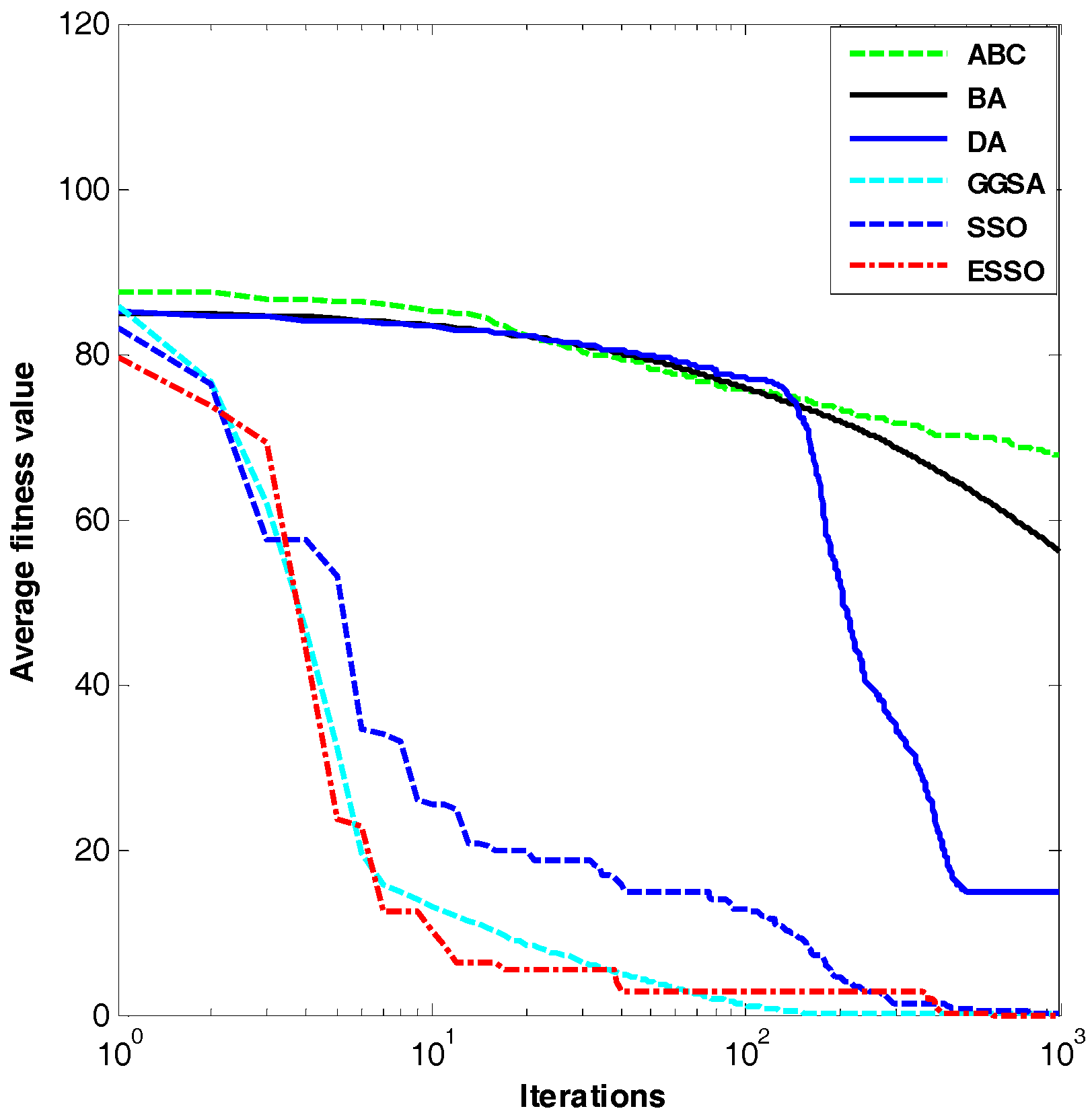
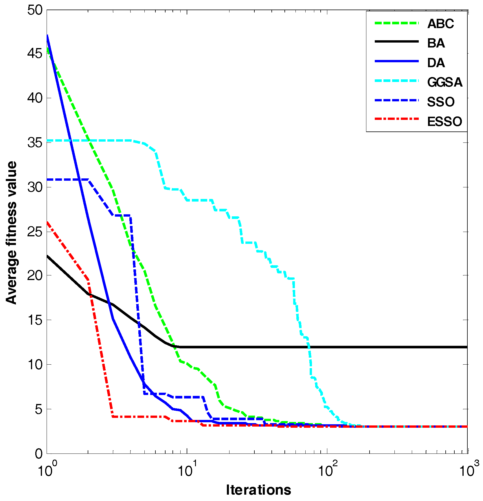
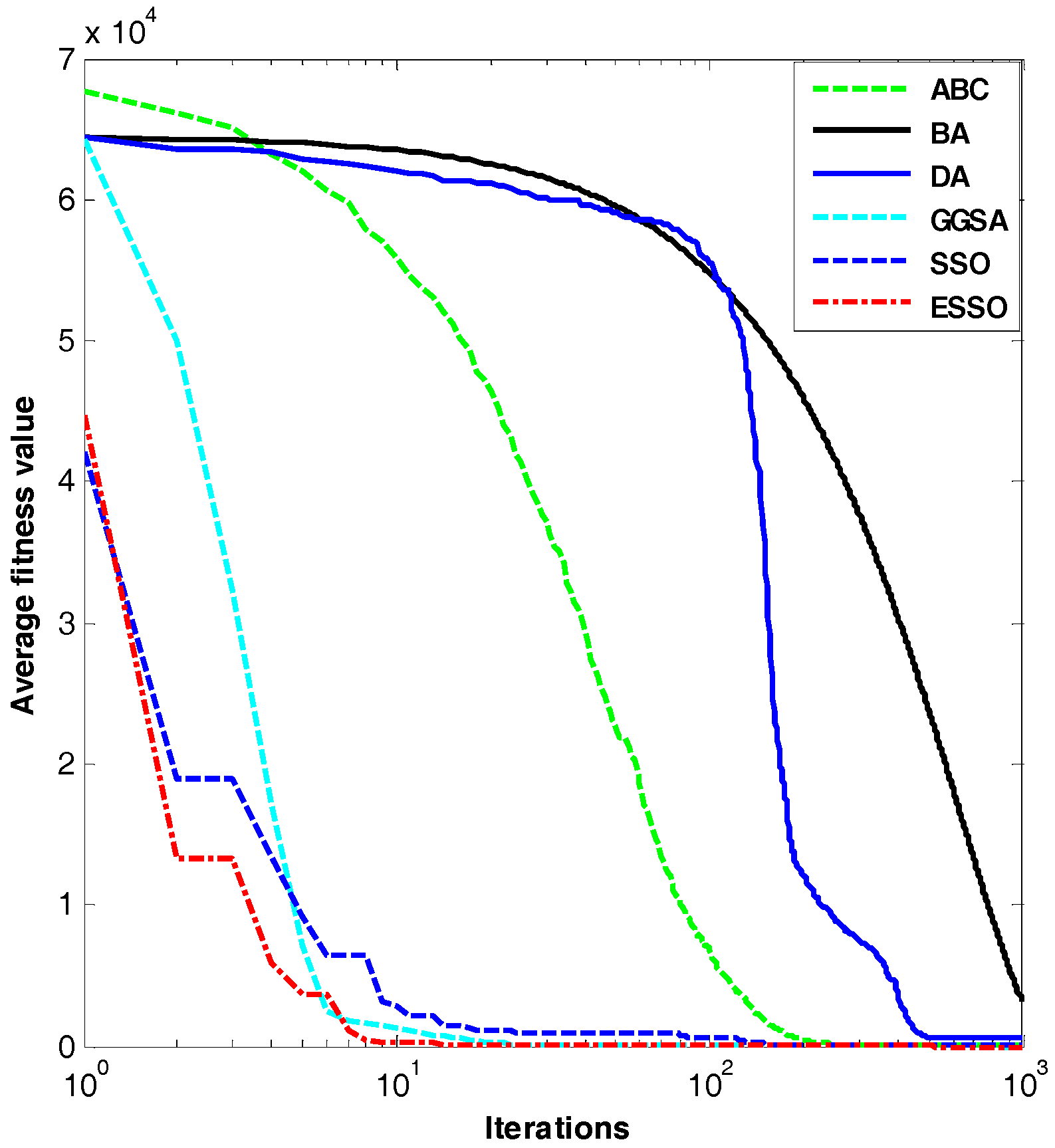
Figure 1.
Dim = 30, evolution curves of fitness value for .
Figure 1.
Dim = 30, evolution curves of fitness value for .
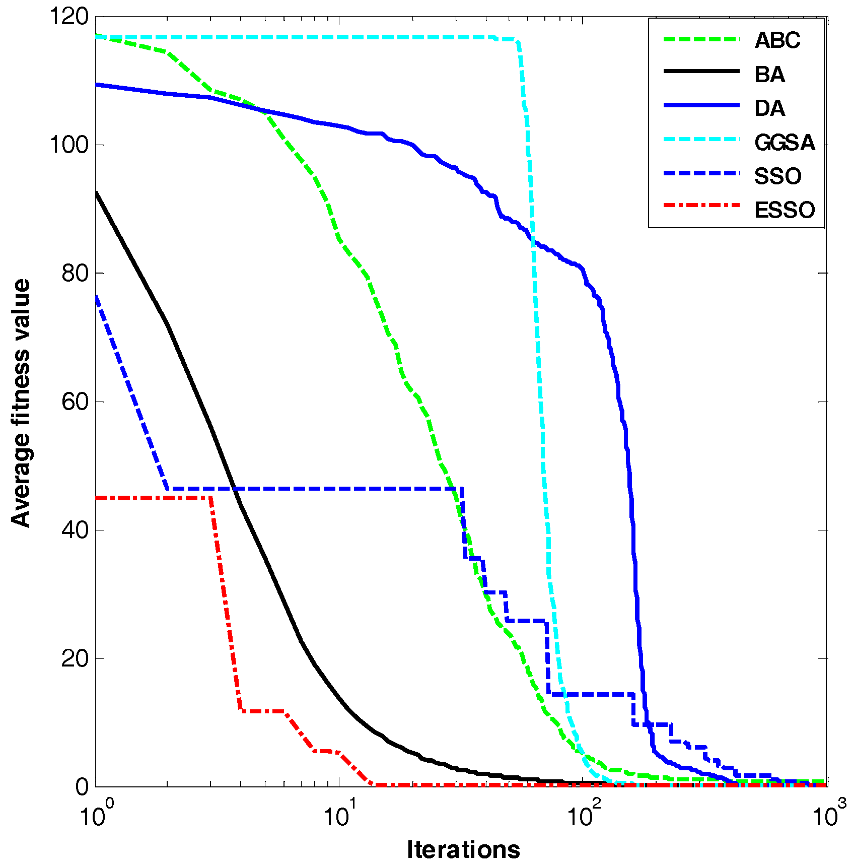
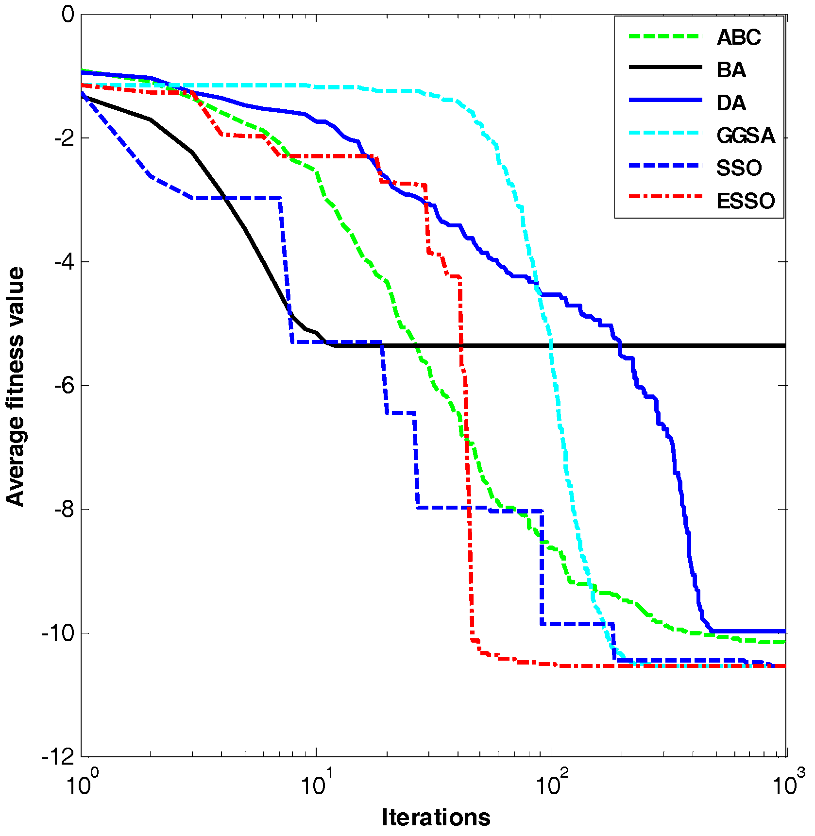
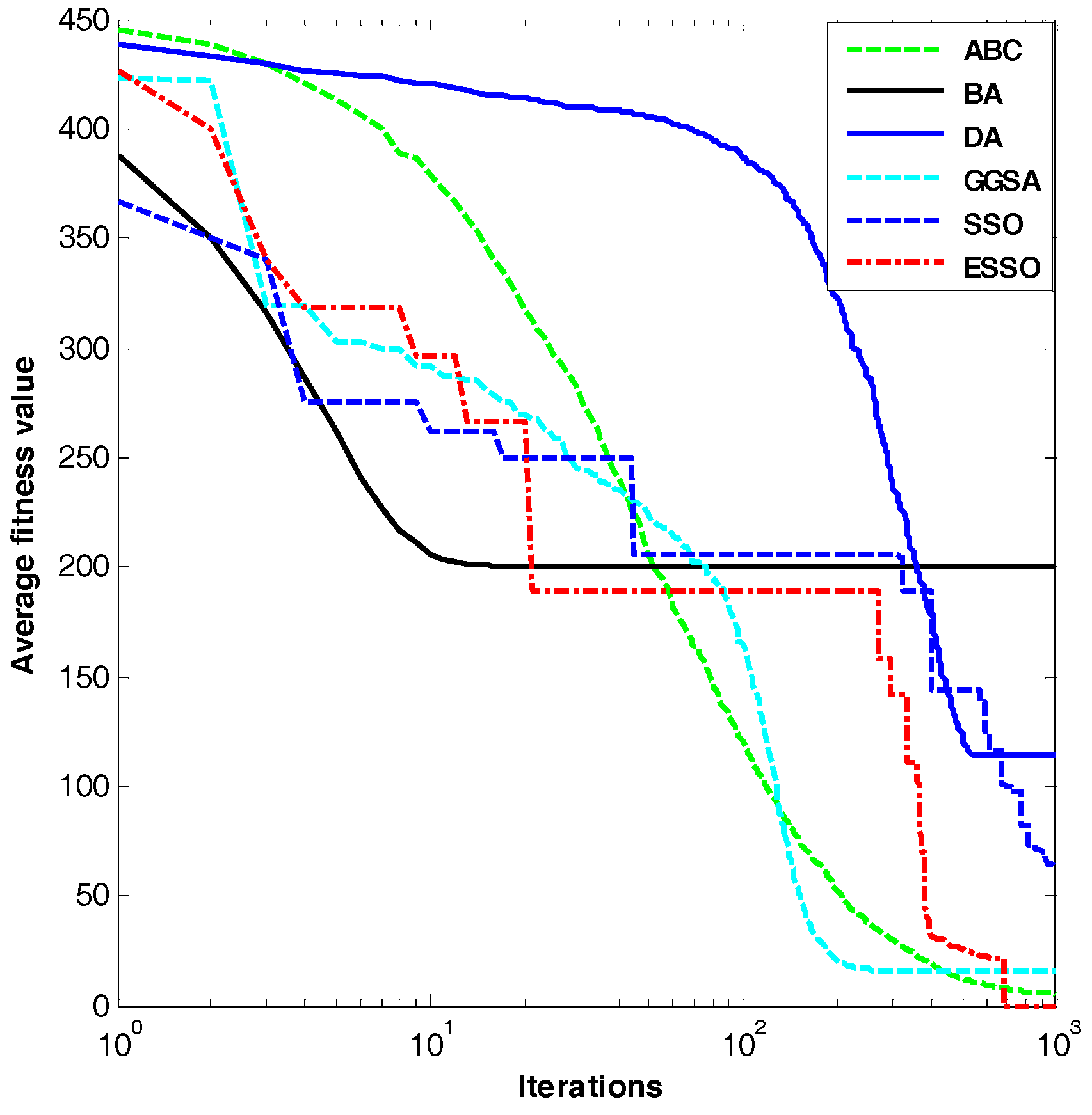
Figure 2.
Dim = 30, evolution curves of fitness value for .
Figure 2.
Dim = 30, evolution curves of fitness value for .
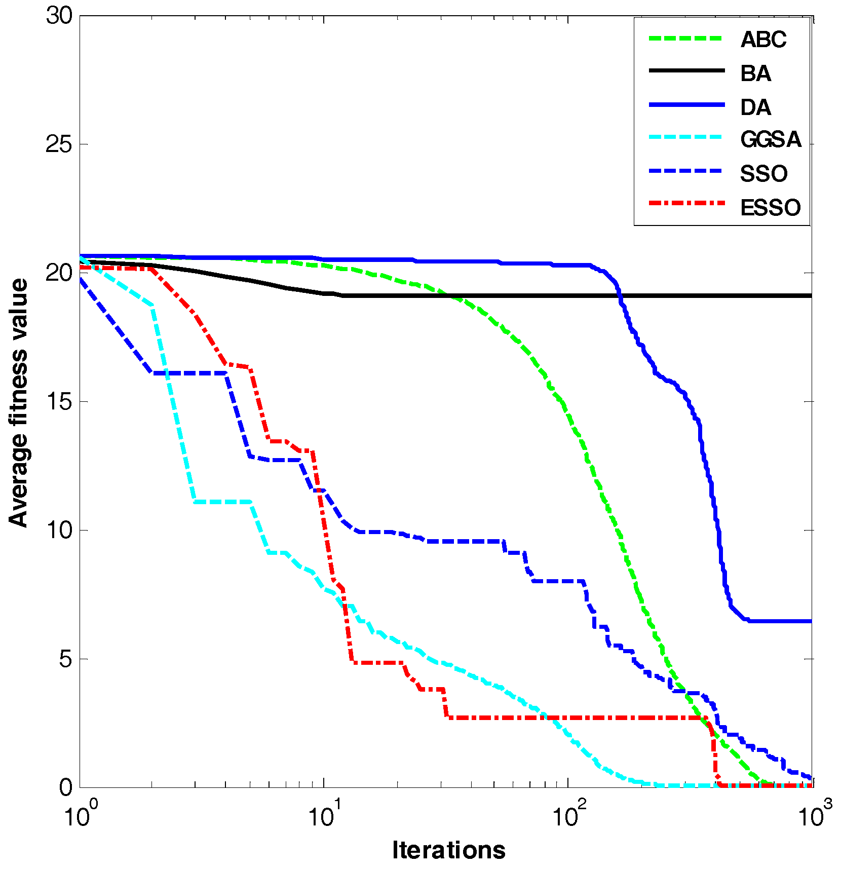
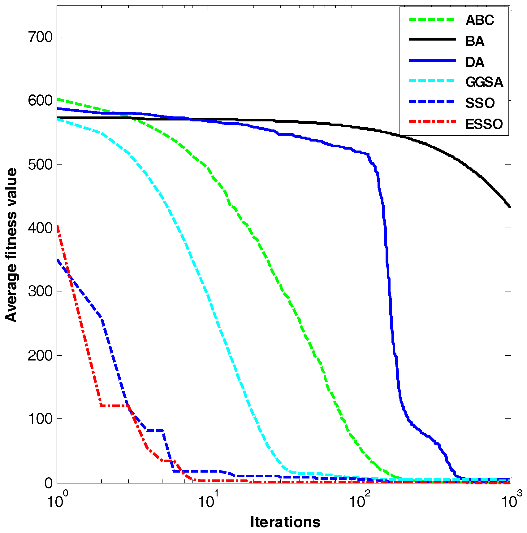
Figure 3.
Dim = 30, evolution curves of fitness value for .
Figure 3.
Dim = 30, evolution curves of fitness value for .
Figure 4.
Dim = 30, evolution curves of fitness value for .
Figure 4.
Dim = 30, evolution curves of fitness value for .
Figure 5.
Dim = 30, evolution curves of fitness value for .
Figure 5.
Dim = 30, evolution curves of fitness value for .
Figure 6.
Dim = 30, evolution curves of fitness value for .
Figure 6.
Dim = 30, evolution curves of fitness value for .
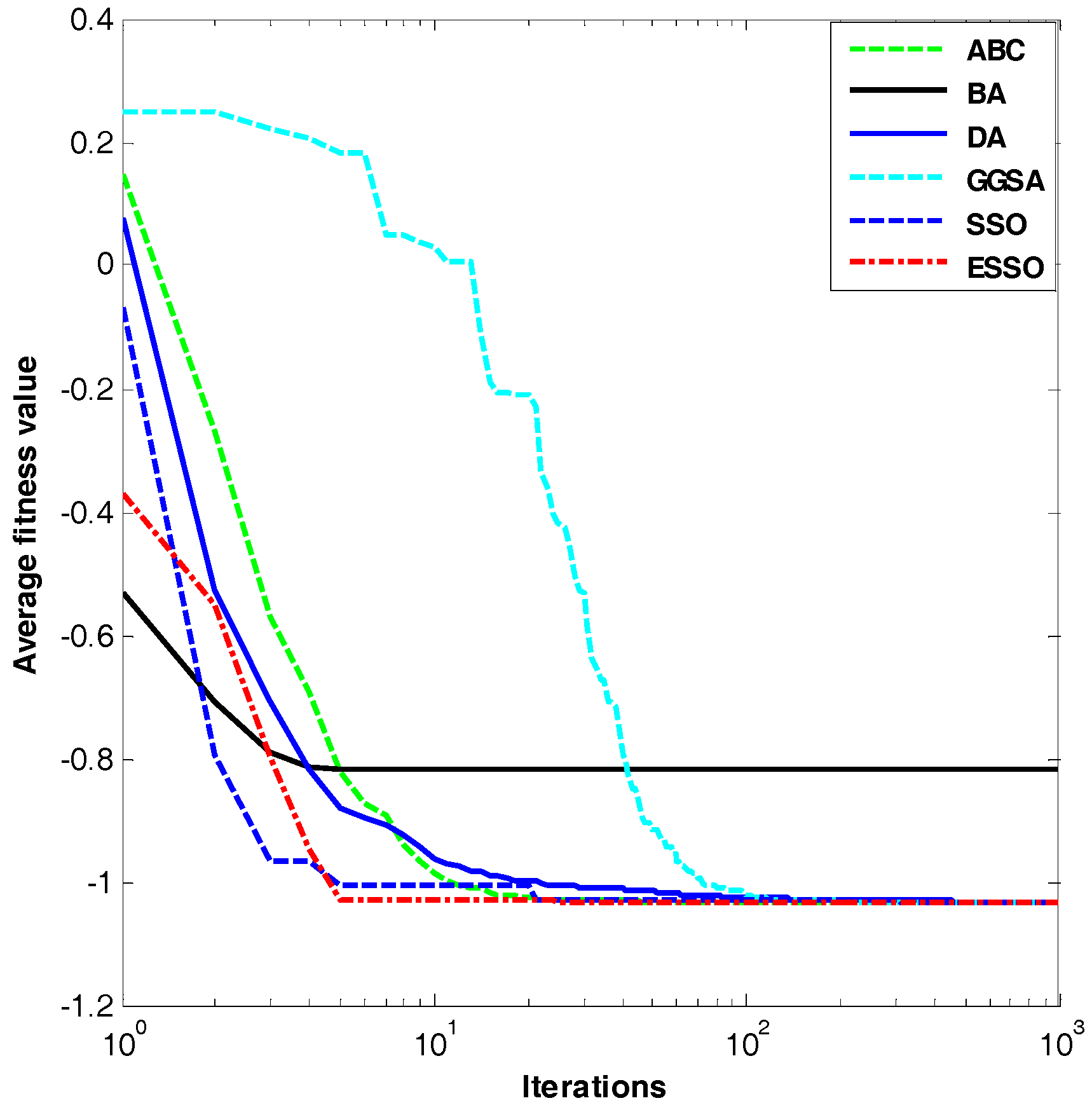
Figure 7.
Dim = 2, evolution curves of fitness value for .
Figure 7.
Dim = 2, evolution curves of fitness value for .
Figure 8.
Dim = 2, evolution curves of fitness value for .
Figure 8.
Dim = 2, evolution curves of fitness value for .
Figure 9.
Dim = 3, evolution curves of fitness value for .
Figure 9.
Dim = 3, evolution curves of fitness value for .
Figure 10.
Dim = 4, evolution curves of fitness value for .
Figure 10.
Dim = 4, evolution curves of fitness value for .
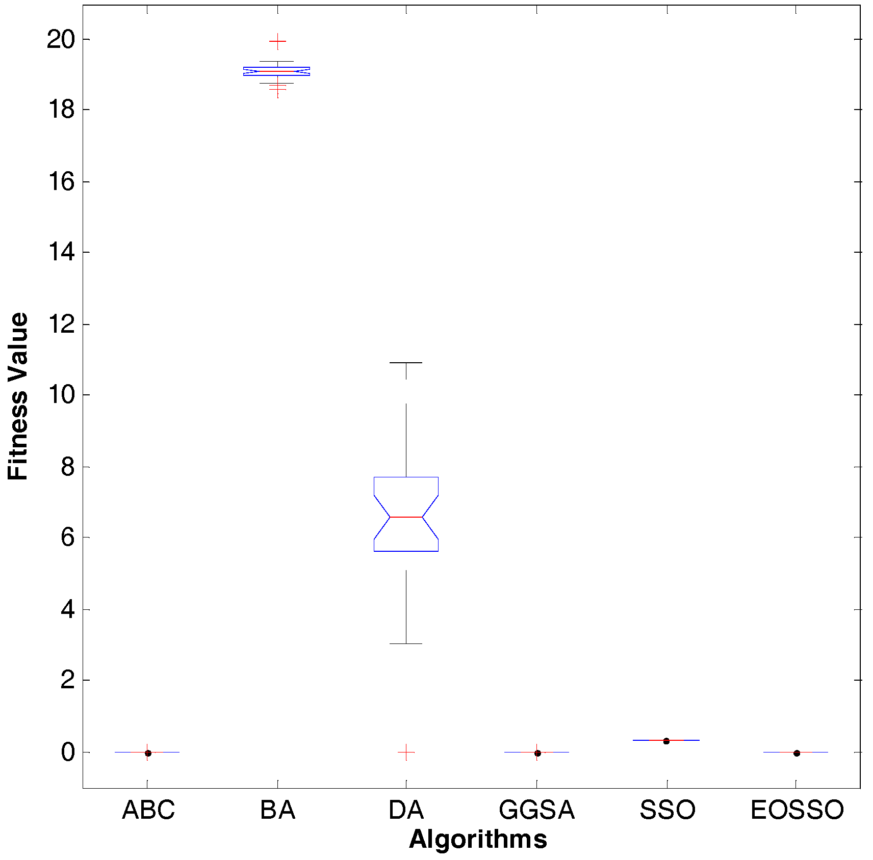
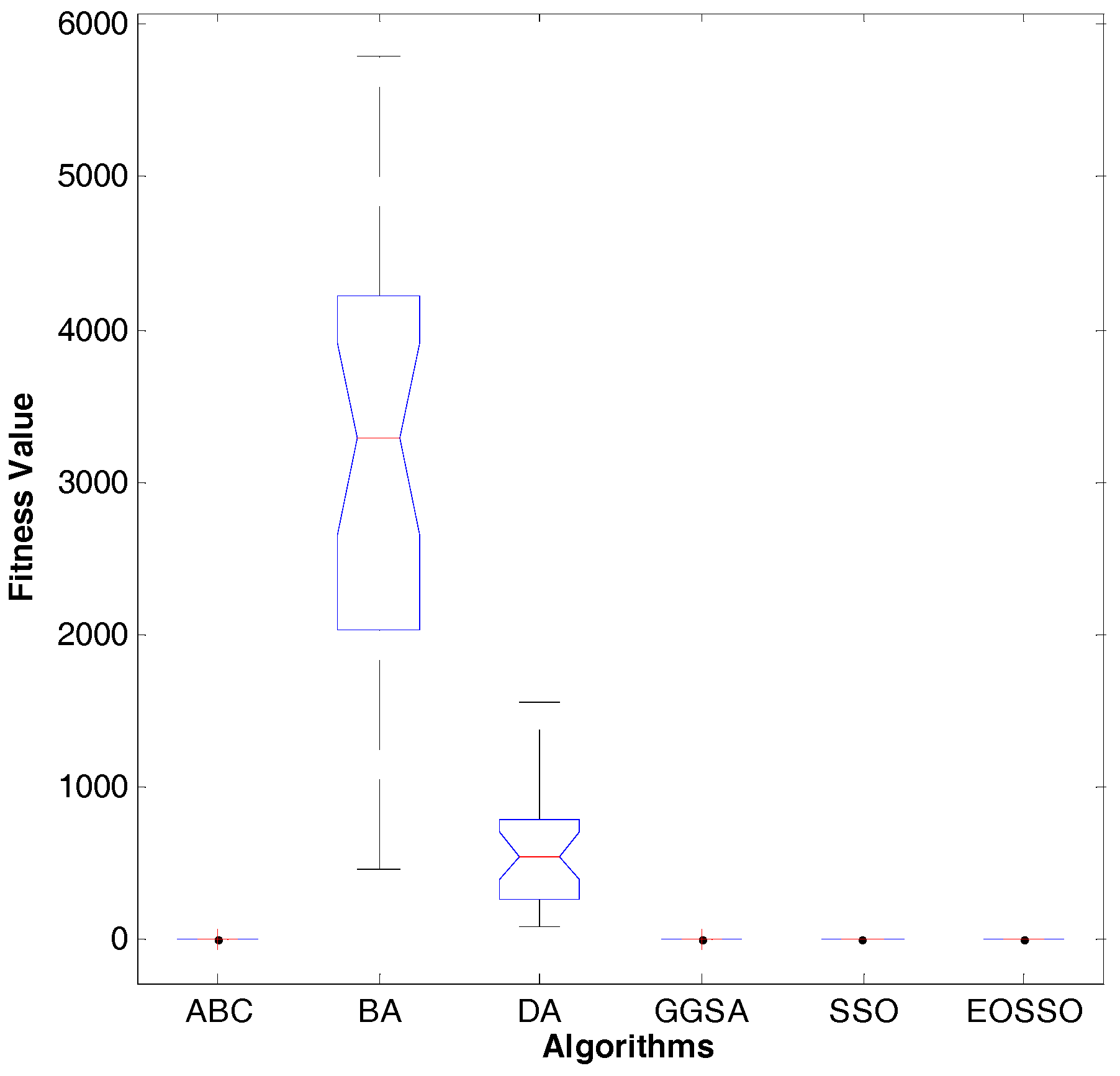
Figure 11.
Dim = 30, variance diagram of fitness value for .
Figure 11.
Dim = 30, variance diagram of fitness value for .
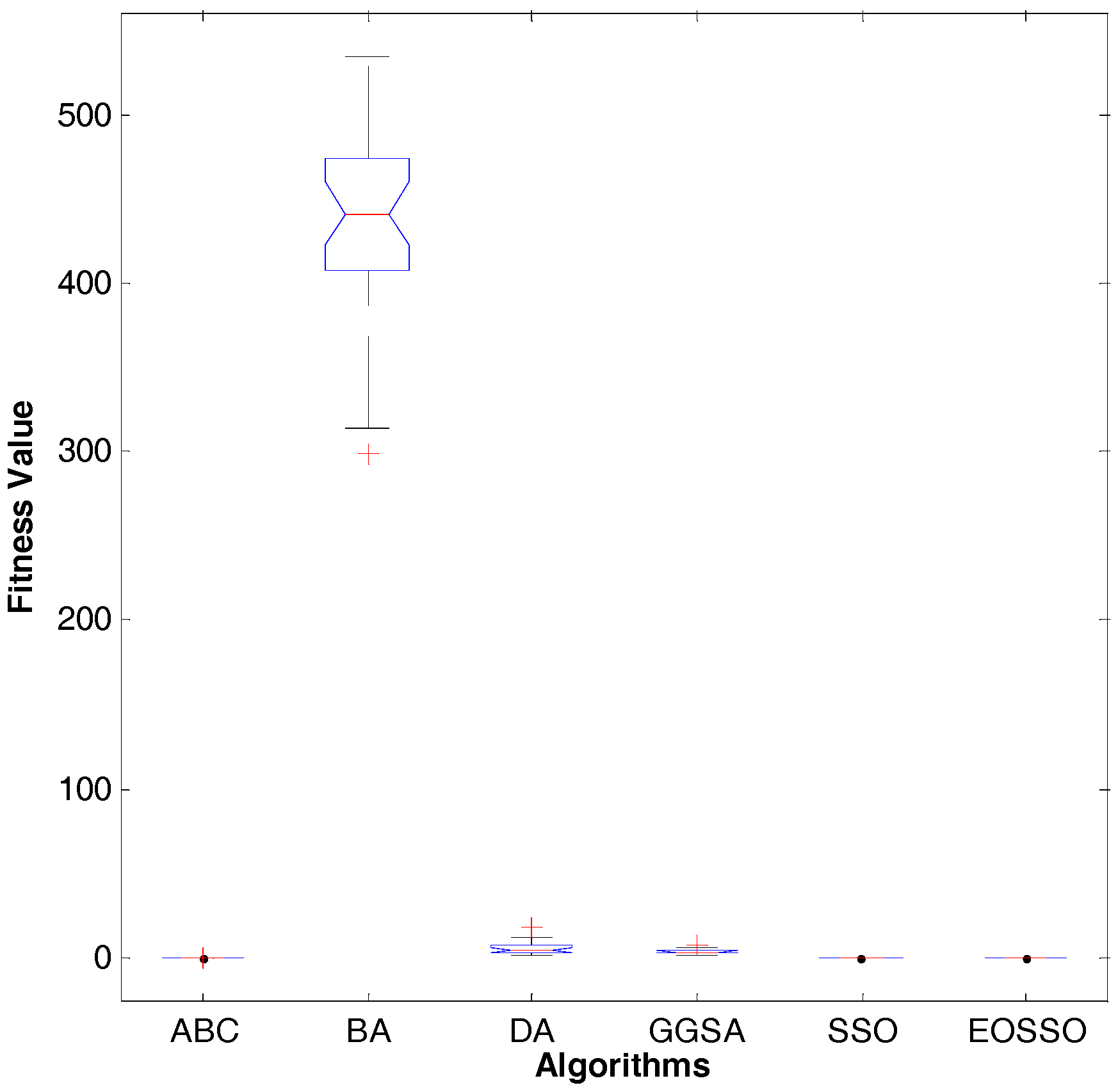
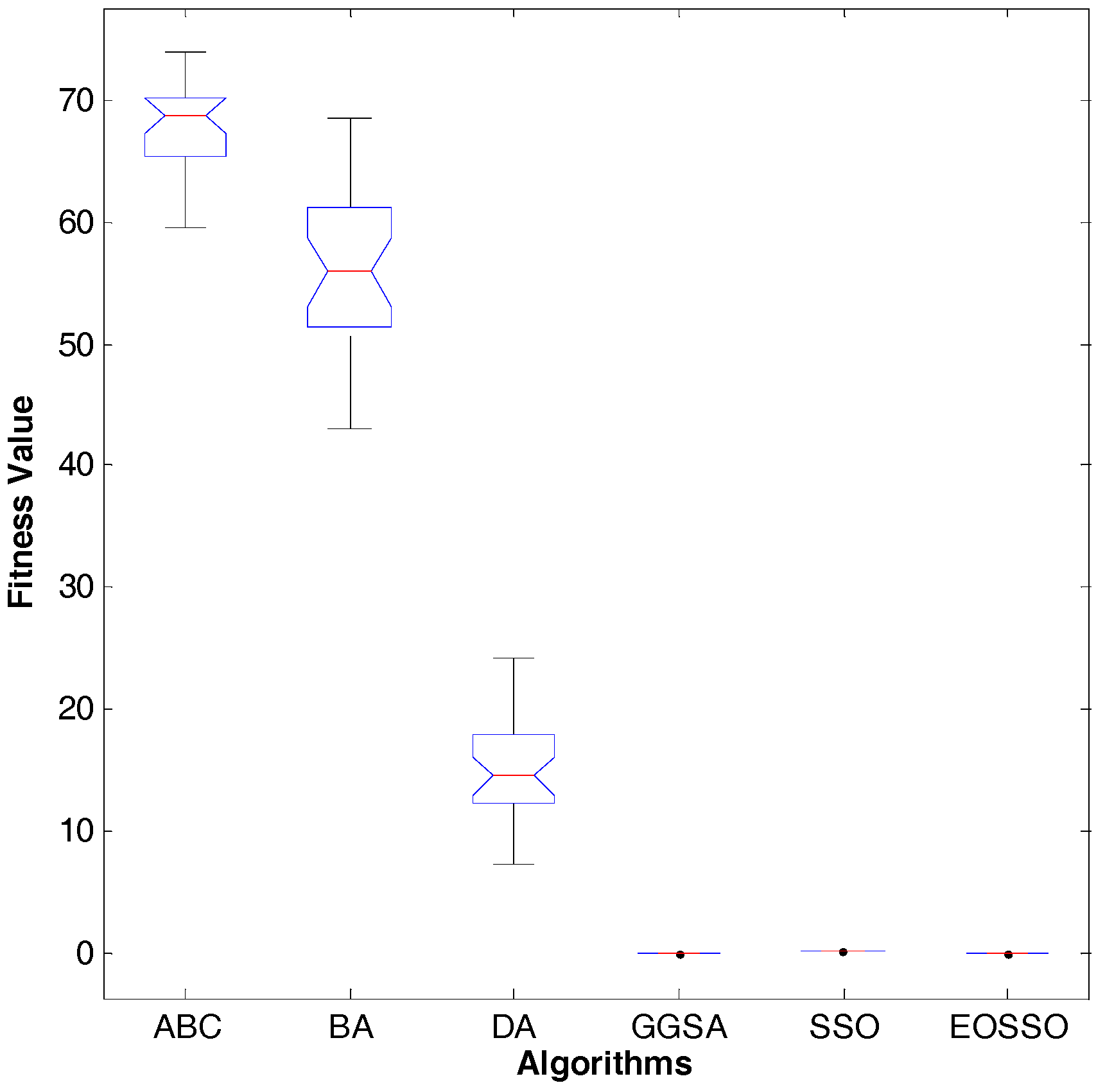
Figure 12.
Dim = 30, variance diagram of fitness value for .
Figure 12.
Dim = 30, variance diagram of fitness value for .
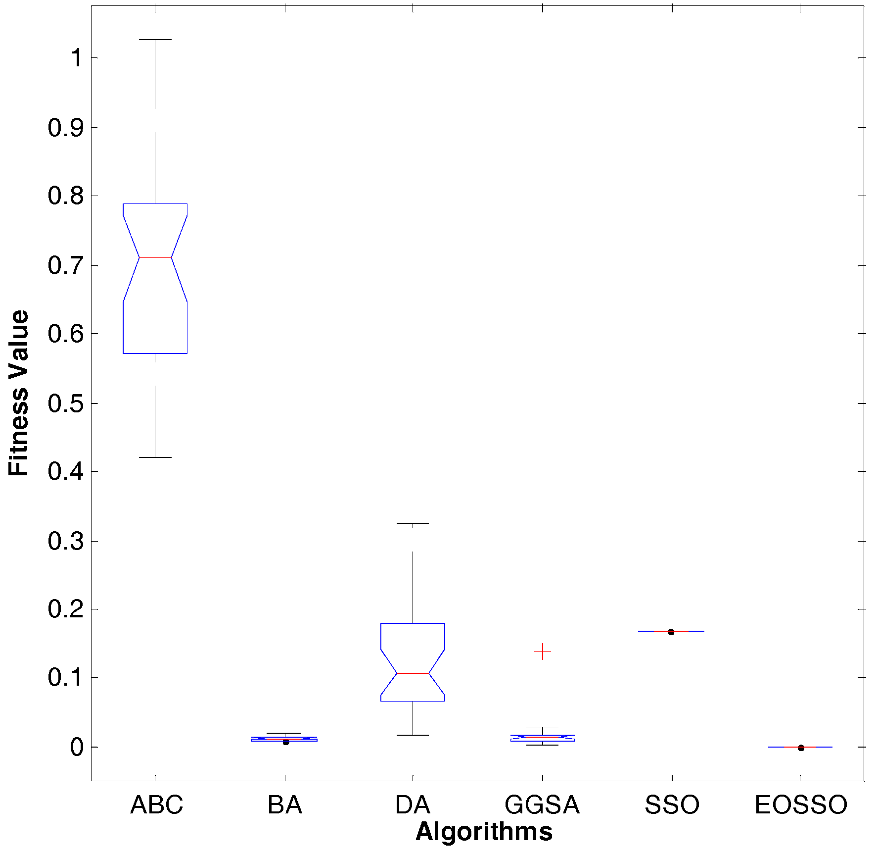
Figure 13.
Dim = 30, variance diagram of fitness value for .
Figure 13.
Dim = 30, variance diagram of fitness value for .
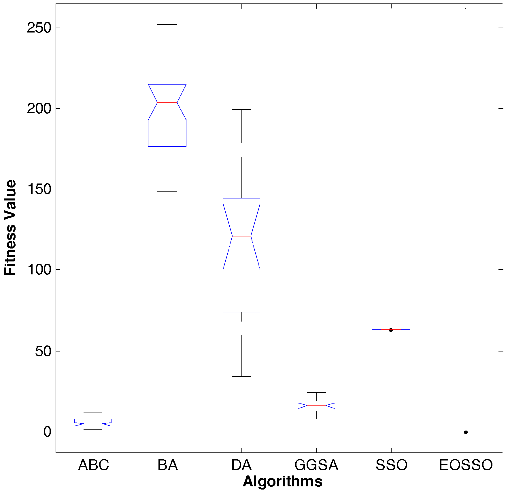
Figure 14.
Dim = 30, variance diagram of fitness value for .
Figure 14.
Dim = 30, variance diagram of fitness value for .
Figure 15.
Dim = 30, variance diagram of fitness value for .
Figure 15.
Dim = 30, variance diagram of fitness value for .
Figure 16.
Dim = 30, variance diagram of fitness value for .
Figure 16.
Dim = 30, variance diagram of fitness value for .
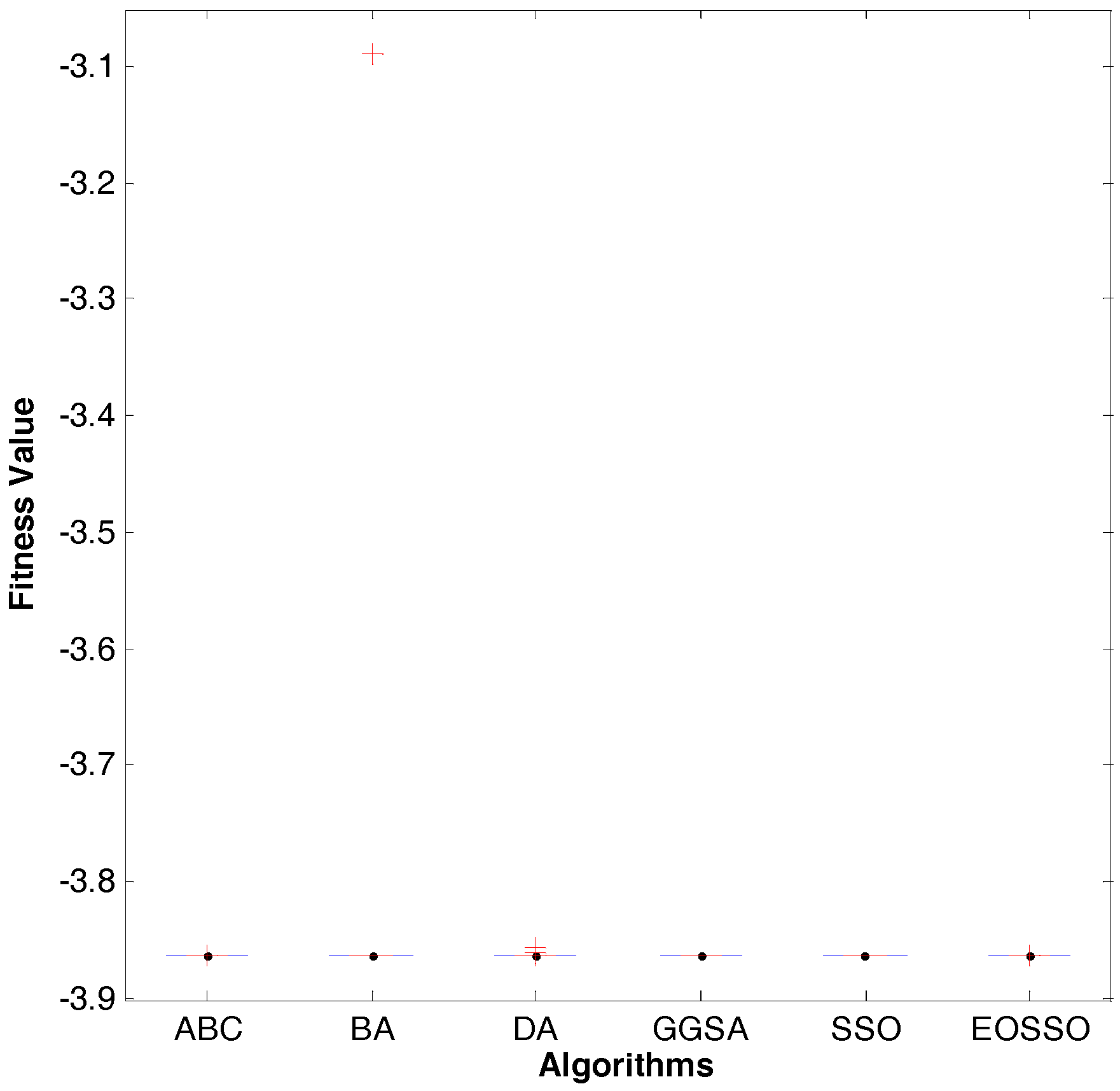
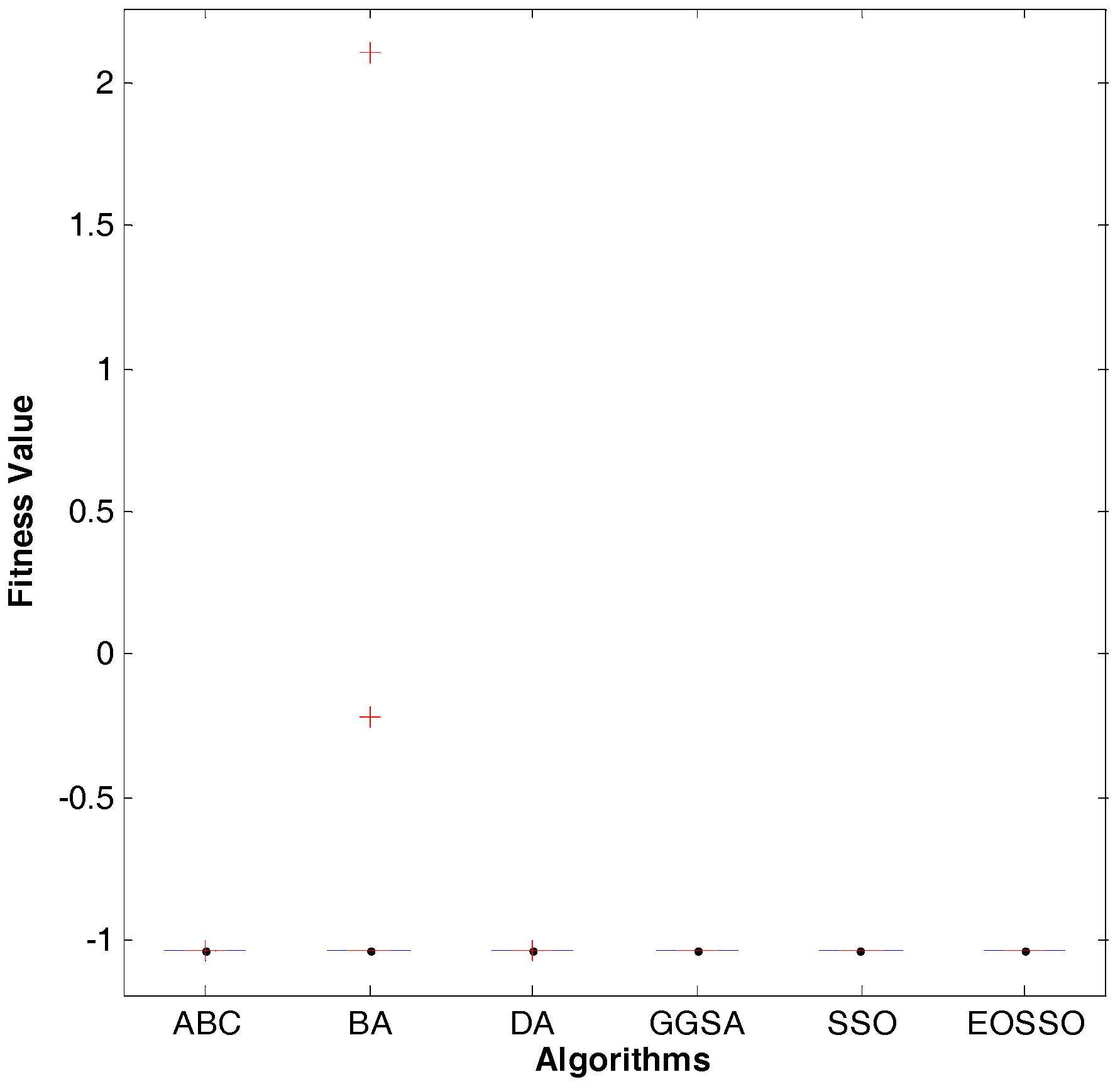
Figure 17.
Dim = 2, variance diagram of fitness value for .
Figure 17.
Dim = 2, variance diagram of fitness value for .
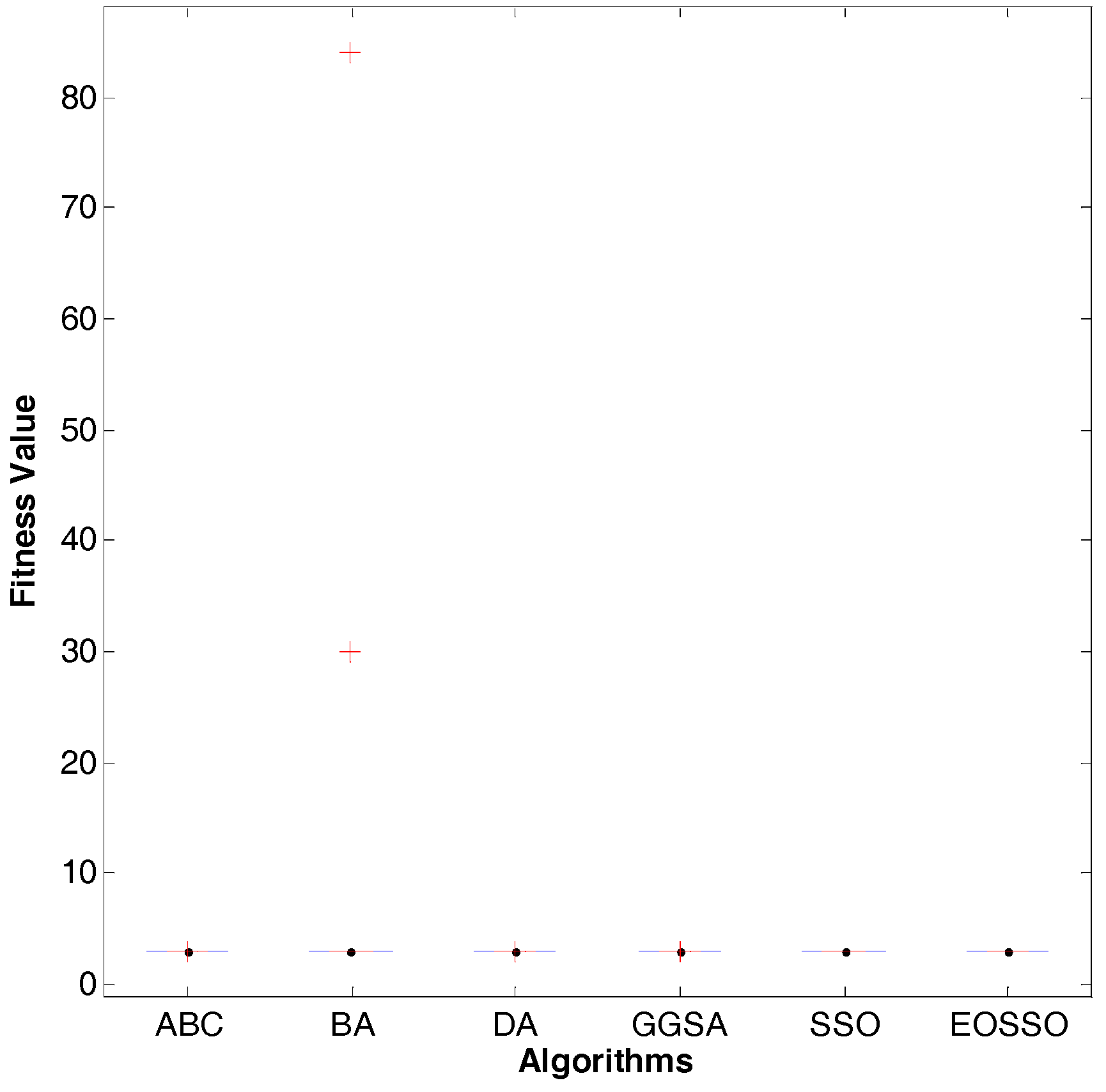
Figure 18.
Dim = 2, variance diagram of fitness value for .
Figure 18.
Dim = 2, variance diagram of fitness value for .
Figure 19.
Dim = 3, variance diagram of fitness value for .
Figure 19.
Dim = 3, variance diagram of fitness value for .
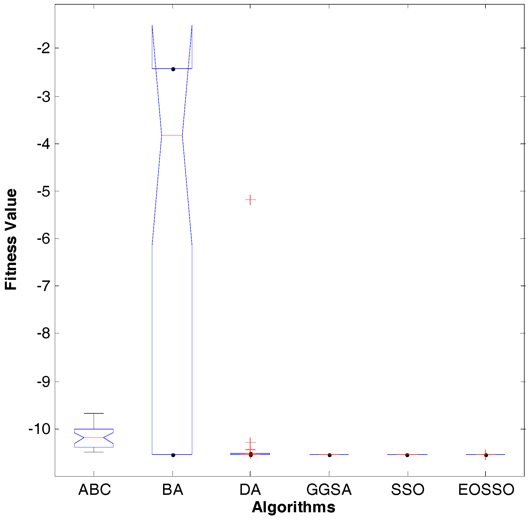
Figure 20.
Dim = 4, variance diagram of fitness value for .
Figure 20.
Dim = 4, variance diagram of fitness value for .
Table 1.
Unimodal benchmark function.
Table 1.
Unimodal benchmark function.
| Function | Dim | Range | fmin |
|---|
| 30 | [−100, 100] | 0 |
| 30 | [−10, 10] | 0 |
| 30 | [−100, 100] | 0 |
| 30 | [−100, 100] | 0 |
| 30 | [−30, 30] | 0 |
| 30 | [−100, 100] | 0 |
| 30 | [−1.28, 1.28] | 0 |
Table 2.
Multimodal benchmark function.
Table 2.
Multimodal benchmark function.
| Function | Dim | Range | fmin |
|---|
| 30 | [−500, 500] | −418.9829*5 |
| 30 | [−5.12, 5.12] | 0 |
| 30 | [−32, 32] | 0 |
| 30 | [−600, 600] | 0 |
| 30 | [−50, 50] | 0 |
| 30 | [−50, 50] | 0 |
Table 3.
Fixed-dimension multimodal benchmark function.
Table 3.
Fixed-dimension multimodal benchmark function.
| Function | Dim | Range | fmin |
|---|
| 2 | [−65, 65] | 1 |
| 4 | [−5, 5] | 0.00030 |
| 2 | [−5, 5] | −1.0316 |
| 2 | [−5, 5] | 0.398 |
| 2 | [−2, 2] | 3 |
| 3 | [1, 3] | −3.86 |
| 6 | [0, 1] | −3.32 |
| 4 | [0, 10] | −10.1532 |
| 4 | [0, 10] | −10.4028 |
| 4 | [0, 10] | −10.5363 |
Table 4.
Simulation results for test unimodal benchmark function.
Table 4.
Simulation results for test unimodal benchmark function.
| Function | Dim | Algorithm | Best | Worst | Mean | std. |
|---|
| 30 | ABC | 3.69 × 10⁻⁸ | 2.32 × 10⁻⁶ | 5.34 × 10⁻⁷ | 5.40 × 10⁻⁷ |
| BA | 4.58 × 10² | 5.79 × 10³ | 3.13 × 10³ | 1.39 × 10³ |
| GGSA | 4.45 × 10⁻²⁰ | 4.17 × 10⁻¹⁹ | 1.72 × 10⁻¹⁹ | 9.49 × 10⁻²⁰ |
| DA | 73.2 | 1.54 × 10³ | 5.50 × 10² | 3.37 × 10² |
| SSO | 8.63 × 10⁻² | 8.63 × 10⁻² | 8.63 × 10⁻² | 0 |
| EOSSO | 3.53 × 10−67 | 3.53 × 10−67 | 3.53 × 10−67 | 2.01 × 10−82 |
| 30 | ABC | 9.47 × 10⁻⁶ | 6.56 × 10⁻⁵ | 2.75 × 10⁻⁵ | 1.27 × 10⁻⁵ |
| BA | 1.14 × 10² | 2.93 × 10⁹ | 1.03 × 10⁸ | 5.35 × 10⁸ |
| GGSA | 8.97 × 10⁻¹⁰ | 3.42 × 10⁻⁹ | 1.88 × 10⁻⁹ | 5.72 × 10⁻¹⁰ |
| DA | 5.81 × 10⁻³ | 20.5 | 8.44 | 52.2 |
| SSO | 1.20 | 1.20 | 1.20 | 2.26 × 10⁻¹⁶ |
| EOSSO | 1.92 × 10−38 | 1.92 × 10−38 | 1.92 × 10−38 | 1.33 × 10−53 |
| 30 | ABC | 1.14 × 10⁴ | 2.45 × 10⁴ | 1.97 × 10⁵ | 3.08 × 10³ |
| BA | 4.33 × 10³ | 1.71 × 10⁴ | 9.12 × 10³ | 3.17 × 10³ |
| GGSA | 1.32 × 10² | 5.37 × 10² | 2.68 × 10² | 90.5 |
| DA | 3.60 × 10² | 1.49 × 10⁴ | 5.39 × 10³ | 3.87 × 10³ |
| SSO | 1.98 | 1.98 | 19.8 | 1.13 × 10⁻¹⁵ |
| EOSSO | 7.61 × 10−76 | 7.61× 10−76 | 7.61 × 10−76 | 6.24 × 10−91 |
| 30 | ABC | 59.6 | 73.9 | 67.8 | 36.2 |
| BA | 42.9 | 68.9 | 56.0 | 65.4 |
| GGSA | 5.25 × 10⁻¹⁰ | 1.96 × 10⁻⁹ | 1.24 × 10⁻⁹ | 4.04 × 10⁻¹⁰ |
| DA | 7.38 | 24.1 | 14.8 | 43.9 |
| SSO | 1.47 × 10⁻¹ | 1.47 × 10⁻¹ | 1.47 × 10⁻¹ | 5.56 × 10⁻¹⁷ |
| EOSSO | 1.20 × 10−37 | 1.20 × 10−37 | 1.20 × 10−37 | 2.12 × 10−53 |
| 30 | ABC | 767 | 89.3 | 37.9 | 20.7 |
| BA | 243 | 5.12 × 10² | 59.4 | 92.4 |
| GGSA | 255 | 1.18 × 10² | 33.0 | 22.0 |
| DA | 30.9 | 2.36 × 10⁵ | 3.41 × 10⁴ | 5.38 × 10⁴ |
| SSO | 35.4 | 35.4 | 35.4 | 0 |
| EOSSO | 26.8 | 26.8 | 26.8 | 1.08 × 10⁻¹⁴ |
| 30 | ABC | 3.43 × 10⁻⁸ | 6.92 × 10⁻⁶ | 1.01 × 10⁻⁶ | 1.67 × 10⁻⁶ |
| BA | 6.99 × 10² | 5.71 × 10³ | 2.82 × 10³ | 1.30 × 10³ |
| GGSA | 0 | 0 | 0 | 0 |
| DA | 1.20 × 10² | 1.56 × 10³ | 4.22 × 10² | 3.16 × 10² |
| SSO | 1.08 × 10⁻¹ | 1.08 × 10⁻¹ | 1.08 × 10⁻¹ | 1.41 × 10⁻¹⁷ |
| EOSSO | 5.01 × 10⁻¹ | 5.01 × 10⁻¹ | 5.01 × 10⁻¹ | 2.26 × 10⁻¹⁶ |
| 30 | ABC | 4.19 × 10⁻¹ | 10.2 | 7.09 × 10⁻¹ | 1.58 × 10⁻¹ |
| BA | 6.93 × 10⁻³ | 2.09 × 10⁻² | 1.23 × 10⁻² | 3.65 × 10⁻³ |
| GGSA | 3.90 × 10⁻³ | 1.39 × 10⁻¹ | 1.73 × 10⁻² | 2.37 × 10⁻² |
| DA | 1.75 × 10⁻² | 3.25 × 10⁻¹ | 1.27 × 10⁻¹ | 8.00 × 10⁻² |
| SSO | 1.68 × 10⁻² | 1.68 × 10⁻² | 1.68 × 10⁻² | 0 |
| EOSSO | 1.22 × 10⁻⁴ | 1.22 × 10⁻⁴ | 1.22 × 10⁻⁴ | 5.51 × 10⁻²⁰ |
Table 5.
Simulation results for test multimodal benchmark function.
Table 5.
Simulation results for test multimodal benchmark function.
| Function | Dim | Algorithm | Best | Worst | Mean | std. |
|---|
| 30 | ABC | −1.21 × 10⁴ | −1.10 × 10⁴ | −1.16 × 10⁴ | 2.81 × 10² |
| BA | −8.45 × 10³ | −5.97 × 10³ | −7.06 × 10³ | 7.40 × 10² |
| GGSA | −3.93 × 10³ | −2.17 × 10³ | −3.08 × 10³ | 3.64 × 10² |
| DA | 7.38 | 24.1 | 14.8 | 4.39 |
| SSO | −7.61 × 10³ | −7.61 × 10³ | −7.61 × 10³ | 2.78 × 10⁻¹² |
| EOSSO | −7.69 × 10³ | −7.69 × 10³ | −7.69 × 10³ | 3.70 × 10⁻¹² |
| 30 | ABC | 1.02 | 11.6 | 5.47 | 2.9 |
| BA | 1.48 × 10² | 2.51 × 10² | 1.99 × 10² | 26.3 |
| GGSA | 7.95 | 23.8 | 16 | 4.57 |
| DA | 34.3 | 1.99 × 10² | 1.14 × 10² | 49.9 |
| SSO | 63.3 | 63.3 | 63.3 | 0 |
| EOSSO | 0 | 0 | 0 | 0 |
| 30 | ABC | 9.16 × 10⁻⁵ | 1.58 × 10⁻³ | 4.79 × 10⁻⁴ | 3.79 × 10⁻⁴ |
| BA | 18.5 | 19.9 | 19 | 2.50 × 10⁻¹ |
| GGSA | 1.48 × 10⁻¹⁰ | 5.26 × 10⁻¹⁰ | 3.09 × 10⁻¹⁰ | 7.42 × 10⁻¹¹ |
| DA | 4.44 × 10⁻¹⁵ | 10.8 | 6.46 | 2.01 |
| SSO | 3.12 × 10⁻¹ | 3.12 × 10⁻¹ | 3.12 × 10⁻¹ | 5.65 × 10⁻¹⁷ |
| EOSSO | 4.44 × 10⁻¹⁵ | 4.44 × 10⁻¹⁵ | 4.44 × 10⁻¹⁵ | 0 |
| 30 | ABC | 2.31 × 10⁻⁷ | 1.34 × 10⁻² | 6.06 × 10⁻⁴ | 2.47× 10⁻³ |
| BA | 2.98 × 10² | 5.34 × 10² | 4.31 × 10² | 60 |
| GGSA | 1.63 | 7.87 | 3.59 | 1.3 |
| DA | 1.56 | 17.5 | 5.05 | 3.4 |
| SSO | 1.26 × 10⁻² | 1.26 × 10⁻² | 1.26 × 10⁻² | 0 |
| EOSSO | 0 | 0 | 0 | 0 |
| 30 | ABC | 1.02 × 10⁻¹⁰ | 1.67 × 10⁻⁸ | 3.32 × 10⁻⁹ | 3.87 × 10⁻⁹ |
| BA | 22.1 | 49.7 | 38.3 | 7.94 |
| GGSA | 4.78 × 10⁻²² | 2.07 × 10⁻¹ | 3.83 × 10⁻² | 6.14 × 10⁻² |
| DA | 1.71 | 52.6 | 12.2 | 12.9 |
| SSO | 1.37 × 10⁻³ | 1.37 × 10⁻³ | 1.37 × 10⁻³ | 2.21 × 10⁻¹⁹ |
| EOSSO | 9.29 × 10⁻³ | 9.29 × 10⁻³ | 9.29 × 10⁻³ | 3.53 × 10⁻¹⁸ |
| 30 | ABC | 1.27 × 10⁻⁸ | 3.55 × 10⁻⁶ | 2.93 × 10⁻⁷ | 6.53 × 10⁻⁷ |
| BA | 80.8 | 1.19 × 10² | 1.04 × 10² | 10.1 |
| GGSA | 5.41 × 10⁻²¹ | 1.09 × 10⁻² | 3.66 × 10⁻³ | 2.00 × 10⁻³ |
| DA | 4.95 | 3.09 × 10⁴ | 1.52 × 10³ | 5.69 × 10³ |
| SSO | 2.04 × 10⁻² | 2.04 × 10⁻² | 2.04 × 10⁻² | 3.53 × 10⁻¹⁸ |
| EOSSO | 6.17 × 10⁻¹ | 6.17 × 10⁻¹ | 6.17 × 10⁻¹ | 3.39 × 10⁻¹⁶ |
Table 6.
Simulation results for test fixed-dimension multimodal benchmark function.
Table 6.
Simulation results for test fixed-dimension multimodal benchmark function.
| Function | Dim | Algorithm | Best | Worst | Mean | std. |
|---|
| 2 | ABC | 9.98 × 10⁻¹ | 9.98 × 10⁻¹ | 9.98 × 10⁻¹ | 1.20 × 10⁻⁵ |
| BA | 9.98 × 10⁻¹ | 22.9 | 10 | 6.97 |
| GGSA | 9.98 × 10⁻¹ | 10.7 | 3 | 2.36 |
| DA | 9.98 × 10⁻¹ | 9.98 × 10⁻¹ | 9.98 × 10⁻¹ | 8.09 × 10⁻¹¹ |
| SSO | 1.99 | 1.99 | 1.99 | 1.36 × 10⁻¹⁵ |
| EOSSO | 9.98 × 10⁻¹ | 9.98 × 10⁻¹ | 9.98 × 10⁻¹ | 4.52 × 10⁻¹⁶ |
| 4 | ABC | 4.16 × 10⁻⁴ | 1.48 × 10⁻³ | 9.93 × 10⁻⁴ | 2.52 × 10⁻⁴ |
| BA | 3.07 × 10⁻⁴ | 5.19 × 10⁻³ | 1.10 × 10⁻³ | 1.17 × 10⁻³ |
| GGSA | 4.80 × 10⁻⁴ | 3.43 × 10⁻³ | 1.78 × 10⁻³ | 6.36 × 10⁻⁴ |
| DA | 4.91 × 10⁻⁴ | 3.44 × 10⁻³ | 1.28 × 10⁻³ | 6.43 × 10⁻³ |
| SSO | 4.18 × 10⁻⁴ | 4.18 × 10⁻⁴ | 4.18 × 10⁻⁴ | 1.65 × 10⁻¹⁹ |
| EOSSO | 3.70 × 10⁻⁴ | 3.70 × 10⁻⁴ | 3.70 × 10⁻⁴ | 2.21 × 10⁻¹⁹ |
| 2 | ABC | −1.03 | −1.03 | −1.03 | 1.25 × 10⁻⁶ |
| BA | −1.03 | 2.1 | −8.18 × 10⁻¹ | 6.19 × 10⁻¹ |
| GGSA | −1.03 | −1.03 | −1.03 | 6.18 × 10⁻¹⁶ |
| DA | −1.03 | −1.03 | −1.03 | 6.27 × 10⁻⁸ |
| SSO | −1.03 | −1.03 | −1.03 | 4.52 × 10⁻¹⁶ |
| EOSSO | −1.03 | −1.03 | −1.03 | 6.78 × 10⁻¹⁶ |
| 2 | ABC | 3.97 × 10⁻¹ | 3.98 × 10⁻¹ | 3.97 × 10⁻¹ | 3.64 × 10⁻⁵ |
| BA | 3.97 × 10⁻¹ | 3.97 × 10⁻¹ | 3.97 × 10⁻¹ | 8.40 × 10⁻⁹ |
| GGSA | 3.97 × 10⁻¹ | 3.97 × 10⁻¹ | 3.97 × 10⁻¹ | 0 |
| DA | 3.97 × 10⁻¹ | 3.97 × 10⁻¹ | 3.97 × 10⁻¹ | 7.62 × 10⁻⁷ |
| SSO | 3.97 × 10⁻¹ | 3.97 × 10⁻¹ | 3.97 × 10⁻¹ | 0 |
| EOSSO | 3.97 × 10⁻¹ | 3.97 × 10⁻¹ | 3.97 × 10⁻¹ | 0 |
| 2 | ABC | 3 | 3.03 | 3 | 8.64 × 10⁻³ |
| BA | 3 | 84. | 12 | 21.6 |
| GGSA | 3 | 3 | 3 | 1.98 × 10⁻¹⁵ |
| DA | 3 | 3 | 3 | 3.28 × 10⁻⁷ |
| SSO | 3 | 3 | 3 | 4.52 × 10⁻¹⁶ |
| EOSSO | 3 | 3 | 3 | 1.81 × 10⁻¹⁵ |
| 3 | ABC | −3.86 | −3.86 | −3.86 | 1.77 × 10⁻⁶ |
| BA | −3.86 | −3.08 | −3.83 | 1.41 × 10⁻¹ |
| GGSA | −3.86 | −3.86 | −3.86 | 2.52 × 10⁻¹⁵ |
| DA | −3.86 | −3.85 | −3.86 | 1.05 × 10⁻³ |
| SSO | −3.86 | −3.86 | −3.86 | 1.36 × 10⁻¹⁵ |
| EOSSO | −3.86 | −3.86 | −3.86 | 4.48 × 10⁻¹⁴ |
| 6 | ABC | −3.32 | −3.31 | −3.32 | 1.03 × 10⁻³ |
| BA | −3.32 | −3.2 | −3.25 | 6.02 × 10⁻² |
| GGSA | −3.32 | −2.81 | −3.29 | 9.71 × 10⁻² |
| DA | −3.32 | −3.07 | −3.26 | 7.34 × 10⁻² |
| SSO | −3.2 | −3.2 | −3.2 | 1.36 × 10⁻¹⁵ |
| EOSSO | −3.32 | −3.2 | −3.2 | 2.17 × 10⁻² |
| 4 | ABC | −10.1 | −9.64 | −9.89 | 1.58 × 10⁻¹ |
| BA | −10.1 | −2.63 | −4.96 | 2.85 |
| GGSA | −10.1 | −5.05 | −5.22 | 9.30 × 10⁻¹ |
| DA | −10.1 | −5.09 | −9.64 | 1.54 |
| SSO | −10.1 | −10.1 | −10.1 | 1.81 × 10⁻¹⁵ |
| EOSSO | −10.1 | −10.1 | −10.1 | 9.70 × 10⁻¹¹ |
| 4 | ABC | −10.3 | −9.78 | −10.1 | 1.90× 10⁻¹ |
| BA | −10.4 | 2.75 | 5.33 | 3.19 |
| GGSA | −10.4 | −5.08 | −7.56 | 2.69 |
| DA | −10.4 | −5.08 | −9.12 | 2.25 |
| SSO | −10.3 | −10.3 | −10.3 | 5.42 × 10⁻¹⁵ |
| EOSSO | −10.4 | −10.4 | −10.4 | 2.02 × 10⁻¹¹ |
| 4 | ABC | −10.4 | −9.67 | −1.01 × 10⁻¹ | 2.06 × 10⁻¹ |
| BA | −10.5 | −2.42 | −5.36 | 3.52 |
| GGSA | −10.5 | −10.5 | −10.5 | 1.32 × 10⁻¹⁵ |
| DA | −10.5 | −5.17 | −9.98 | 1.63 |
| SSO | −10.5 | −10.5 | −10.5 | 3.61 × 10⁻¹⁵ |
| EOSSO | −10.5 | −10.5 | −10.5 | 2.45 × 10⁻¹¹ |


