Article

A Fault Detection and Data Reconciliation Algorithm in Technical Processes with the Help of Haar Wavelets Packets †

Institute of Product and Process Innovation, Leuphana University of Lueneburg, Volgershall 1, D-21339 Lueneburg, Germany
This paper is an extended version of the same author’s paper published in the 2nd International Conference on Advances in Intelligent Systems, Jakarta, Indonesia, 27–28 September 2014.
Algorithms 2017, 10(1), 13; https://doi.org/10.3390/a10010013
Submission received: 30 September 2016 / Revised: 17 December 2016 / Accepted: 7 January 2017 / Published: 14 January 2017

Abstract

:
This article is focused on the detection of errors using an approach that is signal based. The proposed algorithm considers several criteria: soft, hard and very hard recognition error. After the recognition of the error, the error is replaced. In this sense, different strategies for data reconciliation are associated with the proposed criteria error detection. Algorithms in several industrial software platforms are used for detecting errors of sensors. Computer simulations confirm the validation of the presented applications. Results with actual sensor measurements in industrial processes are presented.

1. Introduction

The gross error detection and replacement (GEDR) for many methods based on models or statistics is an important issue in the control field. For instance, a parameter estimation (PE) and data reconciliation (DR) can be taken into consideration very often. At the present time, only a priori noise knowledge based techniques in GEDR are used in industrial applications to detect the outliers that are based on statistical methods. It should be noted that many techniques on the basis of statistical methods could be applied in this context. It becomes more and more essential to clean the data coming from a distributed control system (DCS) because applications in the field of production rely on a great quantity of raw data. Soft sensoring, data reconciliation and parameter estimation need “clean data” [1]. A denoising method based on techniques described in [2] is shown in [3]. This method presented in [4] is based on other methods considered in [2]. The above-mentioned method compares the information theory criterion. A robust version of the Hampel Filter has been developed in [5,6,7]. A new method of de-noising, which is based on methods already introduced in [2], is presented in [3]. It is based on the comparison of an information theory criterion that is the “description length” of the data. In [4,8], this theoretical approach is applied. The description length is calculated for different subspaces of the basis and the method suggests choosing the noise variance and the subspace for which the description length of the data is at a minimum. In the work, based on [4], it is shown that the de-noising process can be done simultaneously. The approach presented in [4,8] is based on “minimum description length” and that’s why it seems to be unsuitable for online detection because it needs a relatively large amount of data. Simultaneous approaches often suffer from the fact that they are based on iterations, which, in turn, impose heavy CPU load requirements on the applications. As a consequence, these approaches often become infeasible for real-time applications, and, therefore, have not been widely used in industry. Real-time approaches dealing with outlier detection and/or de-noising, and featuring easy means of implementation, have also been developed as in [9]. In general, for removing the noise, a lower threshold should be set. This article intends to create an approach treating the outlier detection with denoising in real time without using an a priori noise knowledge technique. Reference [10] demonstrates a procedure that is median function-based, and it is applied in a wavelet-based algorithm. The wavelet-based algorithm proposed in this work is of particular quality due to the adopted a priori noise knowledge free technique. Nevertheless, some misclassifications that may occur are briefly shown at the end of this contribution. The advantage of the presented algorithm consists of its working independently, so no a priori knowledge of the noise level is necessary. Noise level algorithms are considered to be complex and need a great data volume (see [2,3,8]). The advantage of this technique shows that, using a limited stored data, a denoising and fault detection is possible. Figure 1 presents a block diagram of a GEDR package (PCK) interacting with gEST. This paper proposes an algorithm to differentiate discrete signals from their outlier observations using a library of Haar wavelet basis. The algorithm is totally general and can be used in many industrial applications. The effectiveness of the proposed method consists of applying the concept of Lipschitz for using as few samples as possible of the measured signal, and, in the meantime, highlighting the difference between the outliers and the desired signal. The goal is to extract coherent features from the measured signal that will be saved in terms of variance of the Lipschitz constant of the desired signal and outlier signals (or incoherent signal) of which the variance of the Lipschitz constant lies outside this confidential interval. In this sense, the proposed method represents a statistical method that calculates the variance of the Lipschitz constant of the observed signal. The algorithm that has been developed is utilized as a filter to extract features for training neural networks, and it is currently integrated in the inferential modelling platform of the unit for Advanced Control and Simulation Solutions within ABB’s industry division. Industrial applications in fault detection, in which coherent and incoherent signals are univocally visible, are shown.

1.1. Modules

The research of this work is aimed at the gross error detection and replacement (GEDR) and quality module (QM). Nevertheless, the QM is conceptually considered.
  • Process and Instrumentation: The process values can be influenced by sensor aging or incorrect calibration. Biases model effects them, and they are supposed to be smaller in comparison with Gross Errors (GEs).
  • DCS/RTDB (Distributed control system/Real-time database systems): The data logged by DCS/RTDB includes the values from the process and instrumentation block such as noise, outliers and the interference from the measurement; possible effects to the anti-aliasing, analogous digital (AD) conversion, and quantization noise; and possibly LP filtering.
  • Quality Module (QM): DC includes some functions of the QM. In the case of measuring the same physical property by three independent sensors, the value with a “bad” stamp is automatically discarded, and the values of other two sensors will be applied. Other scenarios, including soft sensors, are possible and they depend on the DCS system and configurations. In our case, the QM can bring more performance by means of information from GEDR. Therefore, on input, QM incorporates two streams of information. One of the streams is derived from the DCS/RTDB and the other stream is derived from the GEDR. Properties being referred to the data points combined and gave additional information to other devices: DR, PE, and Data Verification. Series of properties developed by DCS/RTDB can be good/bad, while series of properties developed by GEDR can be replaced/not replaced.
  • GEDR: The data based on the DCS/RTDB block must be elaborated by Gross Error Detection and replacement. The data will be cleared by means of GEDR before proceeding with data (DR) reconciliation (DR) and parameter estimation (PE). The GEs, after being found and deleted, are to be put under analysis made after the DR and PE. It should be done to estimate if they are really GEs and consecutively to configure the filter parameters newly. GE is substituted by GEDR, whose value corresponds to the local behavior of the discovered variable. For this purpose, the average of the last couple of valid data points can be applied. This module is an important part of our research.

1.2. Gross Error Types and Examples

Two types of GEs are taken into account:
  • Type 1 GEs, which are produced by sensor failures and lead to a stable measurement error. Preparation for the detection of type 1 GEs is made. In this case, some user interaction is needed—for example, identifying the number of continuous measurements in type 1 GE. It can succeed for variables such as analyzers, for which clogging may cause such a reaction. In the future, both the number of regular measurements and the dead band must be treated by an expert in this process.
  • Type 2 GEs are caused, for example, by sensor faults, which can have brief, spike-like errors in the measurements as a result.
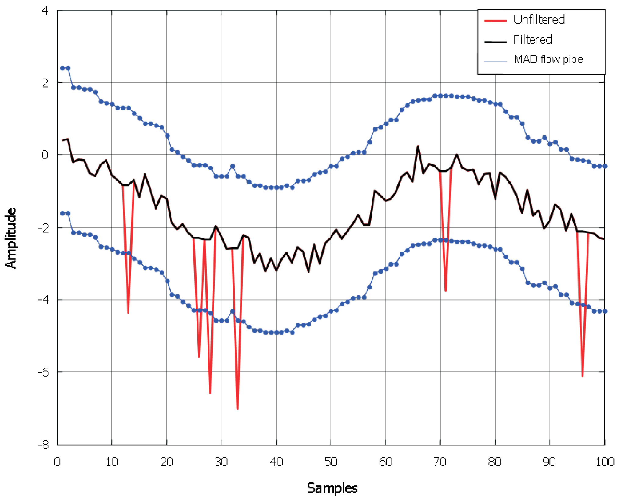
Figure 2 presents the data from a measured temperature, which was contaminated with outliers, and it also presents vague limits min and max temperature, indicated by thick horizontal lines. Some outliers may be easily deleted by the limits. Figure 2 shows data from a temperature measurement contaminated with outliers and hypothetical limits of the min and max values (horizontal thick lines) of the temperature. The limits can be used to perform an easy check to remove some of the outliers. Obviously, not all of the outliers would be removed using the min/max GE check. Another possible easy check could be implemented with a rate limitation. However, this would involve detailed process knowledge of the time constants and noise levels of the measured variables. The GEDR is to remove and replace all of the shown spikes. After detection and replacement, the clean data is shown in the lower part of the figure using a median absolute deviation (MAD) based filter (see [5]), combined together with the wavelet based peak noise level estimation algorithm. Figure 3 shows a graphical representation of the MAD approach with the construction of the MAD flow pipe. This was determined to be the optimal setting, such that the flow pipe is wide enough to accommodate the presence of the noise. However, it is narrow enough to remove a high percentage of outliers. In addition, it can be seen that the “radius” of the flow pipe is invariant under outliers and noise, which, in turn, makes it very robust.
It is clear that not every outlier will be deleted by means of the min/max GE check. There is another possibility of a check which could be applied with a rate limitation. In any case, it requires a deep knowledge on the time constants and noise levels of the variables to be measured. The work presented in [11] is extended by the authors in this contribution. Moreover, some experiments, applying the proposed fault detection method, are considered. This contribution is organized in the following way. Section 2 deals with the problem formulation. Section 4 is devoted to the wavelet based algorithm and some basic definitions of the outliers and evaluation tests. Section 5 considers structured validation evaluation tests of the algorithm. Here, the comparison of the obtained results with another existing algorithm is shown. Finally, industrial application is presented. Finally, conclusions are presented.

2. Problem Formulation

2.1. Mathematical Preliminary

Mathematical Preliminary Measurement errors present a difference between the measured variable and the true value of it:
( y ) k = ( x ) k + ( o ) k + ( b ) k + ( w ) k ,
where ( y ) k is measured, ( x ) k the true value, ( e ) k = ( o + b + w ) k is the error due to the measurement and k denotes the k t h value of the time series. In particular, o k is the outlier, w k is the noise and b k represents any other kind of fault such as, for instance, a sustained error in the measurements, or systematic errors due to the instrumentation. An additive error model similar to an extension of the outlier model presented in [5,12] is also shown in (1). A multiplicative error model in which the errors have been multiplied instead of added is another example of an error model described in the scientific literature. Additive errors are often applied to model errors that occur at the inputs or outputs, while multiplicative errors are applied to model parameter errors (see [5,12]). Consequently, an additive error model is chosen very often. The purpose of the proposed algorithms is associated with the detection of sensor fault related outliers. This leads to a quick GE, characterized by a non-continuous, dynamic response like an impulse or a similar impulse response. Outliers can be differentiated from noise by means of the amplitude of the peaks.

2.2. Outlier Detection Problem (ODP) and Algorithm (ODA)

Consequently, the definition of the outlier index has been made as follows:
Definition 1.
For a set of data ( y ) k = ( x ) k + ( o ) k + ( b ) k + ( w ) k for k = 1 , . . . , n , where ( y ) k is measured. The number of data points n is given. The outlier detection problem (ODP) is to find L = ( l 1 , . . . l n ) for which ( o ) k 0 , that is:
L = ( l ) k = 1 ( o ) k 0 , ( l ) k = 0 e l s e w h e r e .
The index set L itself does not specify what will happen in case of an outlier being actually detected. It is supposed to be a mere specification of the detection problem. ☐
This contribution is not aimed towards proving some of the intrinsic characteristics of a data cleaning filter for solving ODP. It has already been accomplished in [5]. In any case, more definitions are required for assessing the performance of the filter, which is used with the noise detection. Carrying out of the outlier detection algorithm (ODA) will label the data points within the time series ( y ) k that are thought to be outliers. This may be represented by the following definition of a mapping F. The map F becomes a value equal to one, if the considered data point satisfies the criteria, as it was implemented in the Hampel filter in [5].
Definition 2.
For a set of data ( y ) k = ( x ) k + ( o ) k + ( b ) k + ( w ) k for k = 1 , . . . , n where ( y ) k is measured. The number of data points, n, is given. For an implementation of a filter represented by the mapping F, the index vector L T may be computed as follows:
L T = ( l T ) k = 1 ( F ( y ) k ) = 1 , ( l ) k = 0 e l s e w h e r e .
 ☐
This inquiry is principally directed towards the peak noise level evaluation. This is due to the fact that the estimator of the peak noise level reconstructs the noise peaks of the signal and then calculates the variance. In this case, talking about a peak noise level means that the result will be occasionally close to the signal standard deviation, and occasionally closer to the present noise level peak. The aim was to get a robust estimator for a great variety of S/N ratios in the presence of outliers, and then a very accurate estimator for a small range of S/N ratio without outliers. The technique that is considered is based on the wavelets. The local variance of the Lipschitz constant of the signal over a sliding time horizon is evaluated by the implemented algorithm. In case of the local Lipschitz being constant lying outside the computed limit, the outlier is identified. A flow pipe for the Lipschitz constant is graphically produced and if the local Lipschitz constant is situated outside the flow pipe, the data point is marked, and, after that, it is substituted.

3. Short Remarks on Haar Wavelets

Wavelets are mathematical functions that are based on time frequency. They analyze physical situations with the signal containing discontinuities and sharp spikes better than traditional Fourier Methods. Wavelets are very often applied in mathematics, quantum physics and electrical engineering. Intersection between these subjects in the last decade caused increasing wavelet applications such as image compression, turbulence, human vision and radar. Currently, Digital Signal Processors implement sampled signals. Only approximated values of the signal projection coefficients can be often calculated by selecting a particular signal approximation. A great number of wavelet functions that have different features exist, and, a short time ago, polynomial structures started to be applied for creating wavelets. In [13], a wavelet having a form of a cubic spline is presented in pre-filtering applications. Haar wavelets have a wide application field in industry. Representation of discrete signals using Haar wavelets is very compact due to the use of microprocessors (see [14]). A brief overview on the Haar wavelets function ψ ( d , j , n ) ( t ) = ψ j ( 2 d t n ) is considered with a support of size 2 d of the Nyquist frequency. Furthermore, d is a scale parameter, j is a phase parameter and n is a time translation parameter. Here, the pyramidal packet is represented by the indices ( d , j , n ) , d is the level of the tree (scaling parameter), j is the frequency cell (oscillation parameter) and n the time cell (localization parameter). Basically, the Haar basis has the following two properties:
  • the ψ ( d , j , n ) h ( t ) are orthonormal,
  • any L 2 ( ) function f ( t ) can be approximated, up to arbitrarily low precision, by a finite linear combination of the ψ ( d , j , n ) h ( t ) .
In particular, to be more precise, coefficients w ( d , j , n ) (the weight coefficients) are calculated as follows:
w ( d , j , n ) = I f ( t ) ψ ( d , j , n ) h ( t ) d ( t ) .
For j = 0 , it is possible to define the following coefficients:
s ( d , 0 , n ) = I f ( t ) ψ ( d , 0 , n ) h ( t ) d ( t ) ,
where f ( t ) is the required signal, I is the considered time interval and ψ ( d , 0 , n ) h ( t ) is the well-known mother function. To conclude:
f ( t ) = n s ( d , n ) ψ ( d , 0 , n ) h ( t ) + j n w ( d , j , n ) ψ ( d , j , n ) h ,
where s ( d , n ) = w ( d , 0 , n ) . It is shown that there are just two independent parameters and that parameter d characterizes the level of the tree. The wavelet packets under consideration are derived from the Haar mother wavelet.
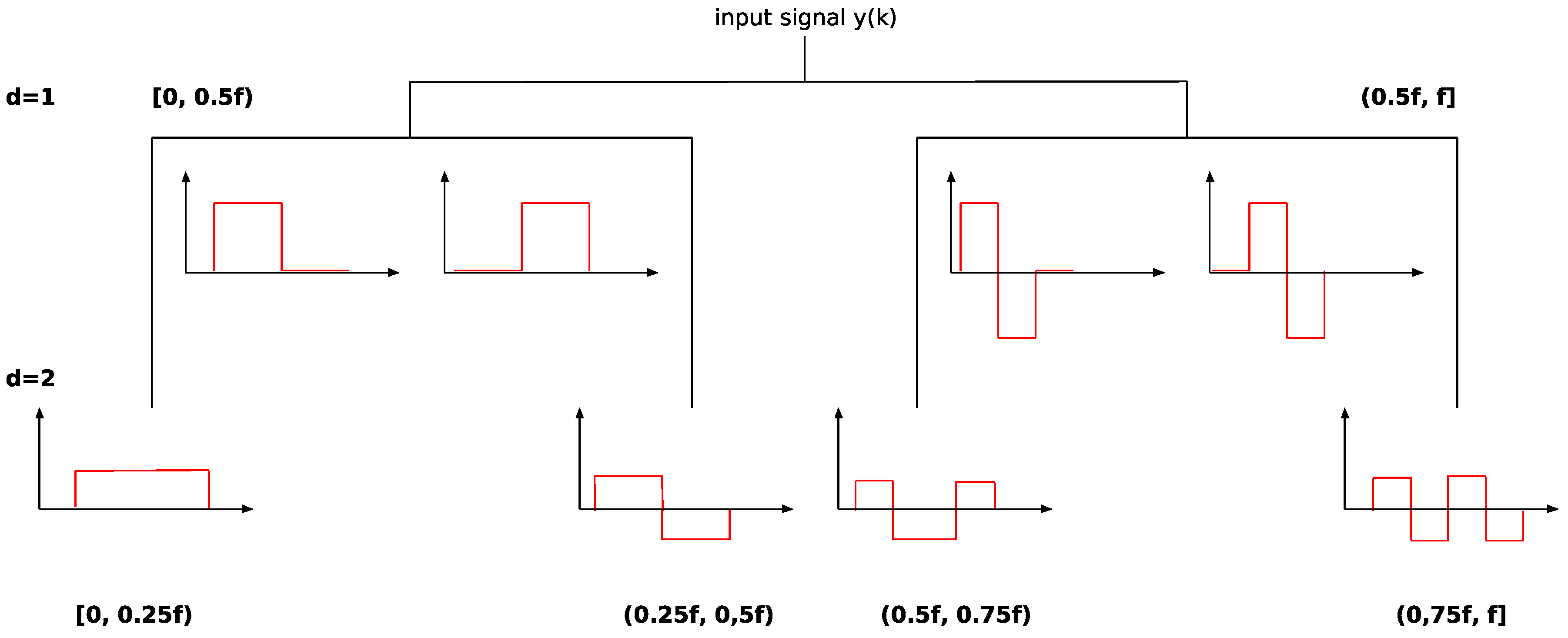
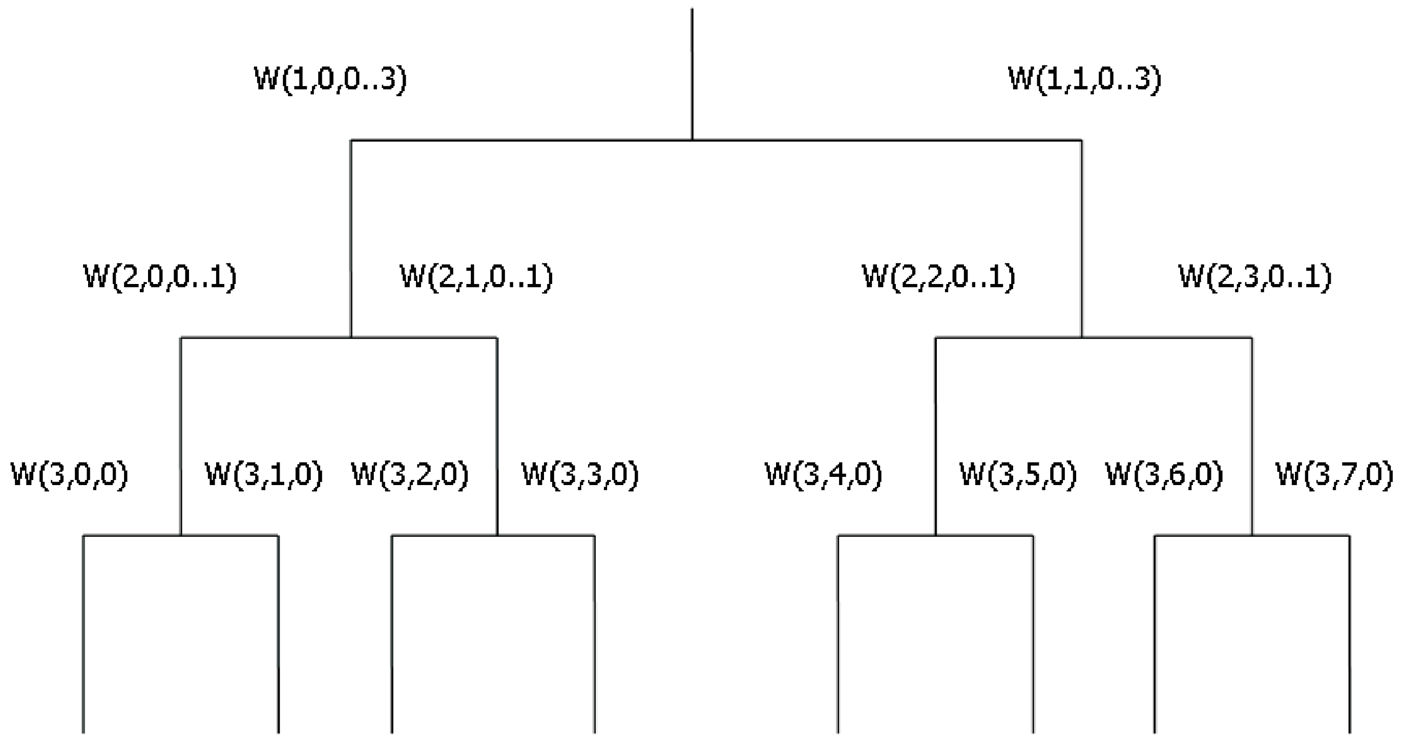
A set of Haar functions are presented in Figure 4. The localisation of the Haar functions through the tree is accomplished by means of the parameter tuple, ( d , j , n ) , as shown in Figure 4. Moreover, there is a relation of parameter j to the frequency shift, a relation of parameter n to the time shift, and the supplementary parameter d is necessary to address the level of the tree directly depending on the number of the examined samples. It means that if eight samples are to be considered, the level of the tree will be three. Wavelet functions are constructed like a tree, so d = 1 is the highest degree of improvement concerning the time. Figure 4 demonstrates four wavelet functions at d = 1 and the four wavelet functions for d = 2 . The appropriate coefficients, w ( d , j , n ) representing the wavelet functions, for a tree consisting of d = 3 is shown in the right part of Figure 5. w ( 1 , 0 , 0 . . 3 ) indicates the coefficients of the first level on the extreme left with time shifts 0 through 3. One of the motivations to choose Haar wavelets is that they are the most structurally simple wavelets to be applied. This means that, with a window of four samples, we can already achieve very good results. This is not the same for other wavelet families because of higher vanishing moments, and some wavelet families are available for application starting with a window of 16 samples. This represents a drawback. In fact, using a long window, the actuality of the information is lost. Another reason to use Haar wavelet family is that, because of the application in micro-controllers, the discrete shape of the signals can be represented basically as a combination of Haar functions. This represents an advantage because the compression of the signal into the Haar basis is a very compact one and can be very useful in the case of localisation of disturbances or identification of dominant or subdominant harmonics.

4. The Proposed Algorithm and Its Verification

Fault evaluation is an important problem both in theory and in practice. Works dedicated to this topic are considered in [15,16]. Some various methods for choosing fitting threshold values have been introduced. The presently applied algorithms used to evaluate the faults with the help of wavelets could be summed up as follows:
  • Obtain the coefficients by applying the Haar wavelet transform to the signal affected by faults;
  • Threshold those elements in the wavelet coefficients, which are considered to refer to faults;
  • Replace the fault in the considered sequence.
The most important point in this approach is represented by the threshold step, which is when wavelet coefficients are supposed to refer to the fault. The fault (outlier) is determinate in case of the local Lipschitz constant being external with respect to the calculated boundary. Two confidential constants are denoted by parameters c 1 and c 2 . A short version of this algorithm is also published in [17], but an analysis in terms of soft, hard and very hard thresholding is done in this paper.

Structure of the Algorithm

  • Step 1 The signal is located in a register and the standard σ of the local Lipschitz (L) constant of its first seven samples is computed by means of the scalar product between two consecutive samples and Haar functions having two samples. Subsequently, one calculates the local Lipschitz constant considering the 7th and 8th sample correspondingly.
  • Step 2a In case of the local Lipschitz constant being calculated considering the 7th and 8th sample of signal which is less than constant c 1 σ , the examined element of the sequence is not an outlier and the local Lipschitz constant is summed up with σ.
  • Step 2b In case of the local Lipschitz constant computed considering the 7th and 8th sample being bigger than constant c 1 σ , then the examined element of the sequence is an outlier and its local Lipschitz constant is not saved. The case of single outliers is reported in Figure 3.
  • Step 3 The local Lipschitz constant is saved and the next step of the sequence is taken under consideration.
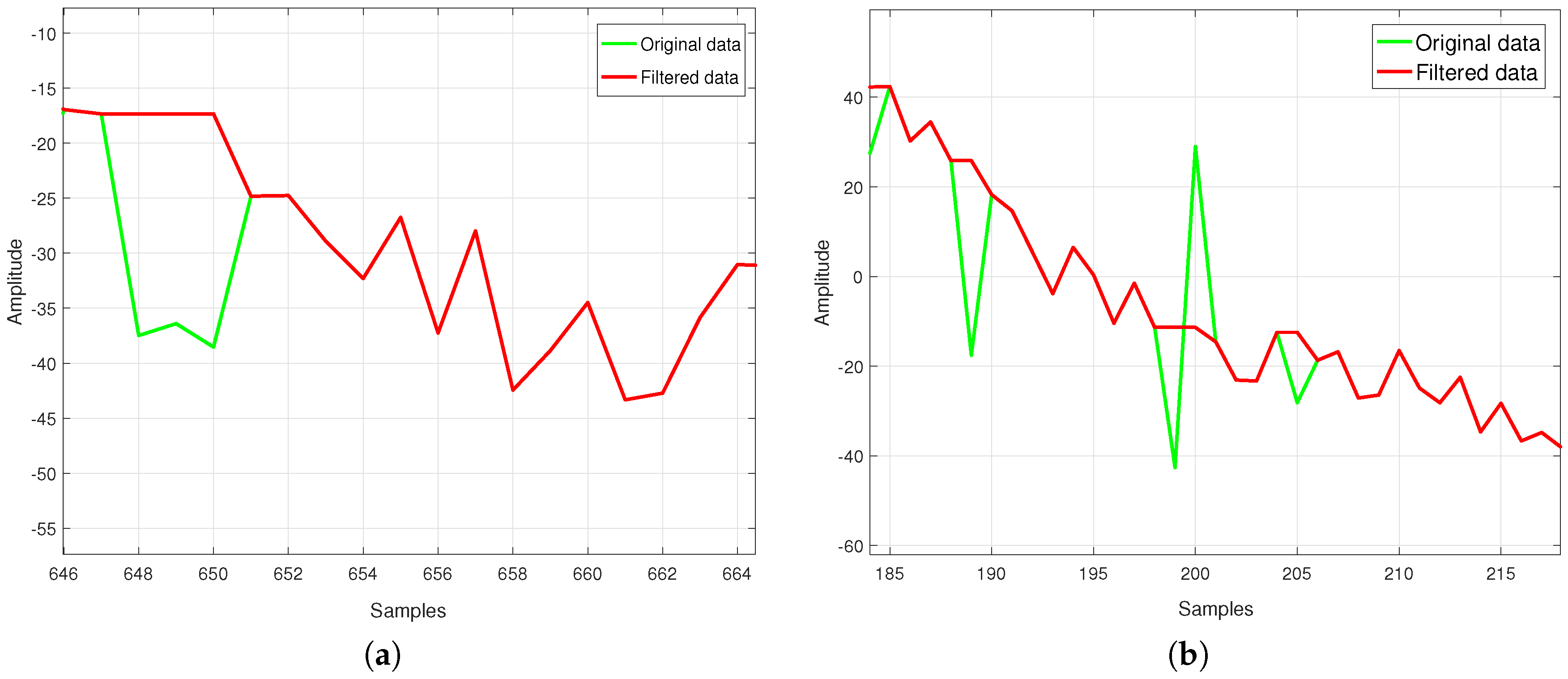
  • Step 4 If the saved local Lipschitz constant value is bigger than c 1 σ , then the sign of the last two computed local Lipschitz constants is analyzed. In case of their not being opposite signs, multi-outliers appear (see Figure 6a).
Assuming that they are opposite signs, the saved local Lipschitz constant value is checked. In the case that this value is not less than c 2 σ , it results in being a single inverse outlier, as it can seen in Figure 6b.
Remark 1.
With help of this algorithm, it is possible to accomplish soft, hard and very hard fault detection strategies simply by choosing parameters c 1 and c 2 together with the replacing term, if an outlier (fault) appears. For c 1 = 1 and c 2 = 2 , together with
R e p l a c e d = E l e m e n t ( k 1 ) + ( O u t l i e r E l e m e n t ( k 1 ) ) 2 ,
a soft detection is obtained. For c 1 = 0.5 and c 2 = 1 , together with
R e p l a c e d = E l e m e n t ( k 1 ) + ( O u t l i e r E l e m e n t ( k 1 ) ) 2 ,
a hard detection is obtained. For c 1 = 0.5 and c 2 = 1 , together with
R e p l a c e d = E l e m e n t ( k 1 ) ,
a very hard detection is obtained.

5. Results

The evaluation of the procedure is made by means of artificial data in which the positions of the outliers are given.
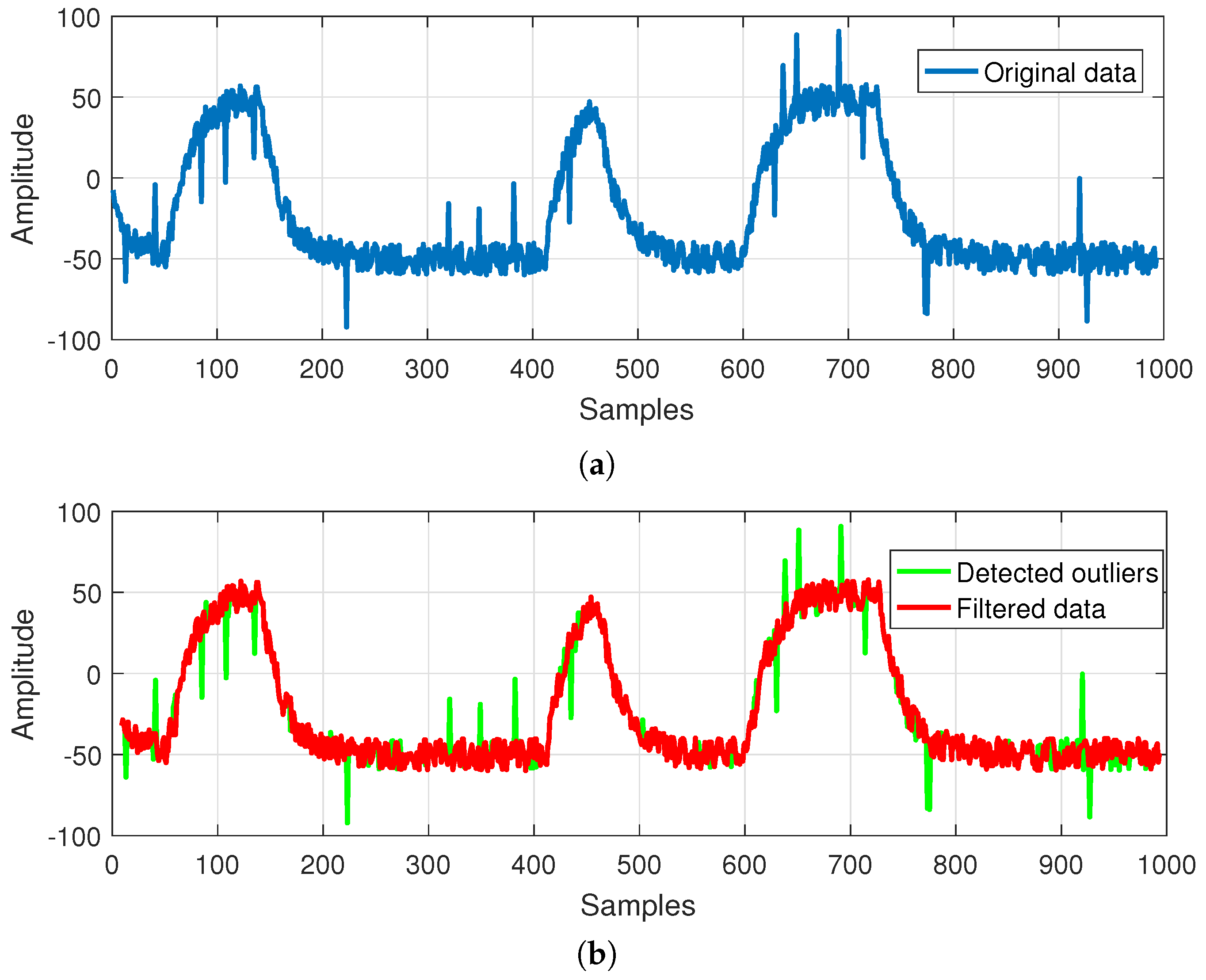
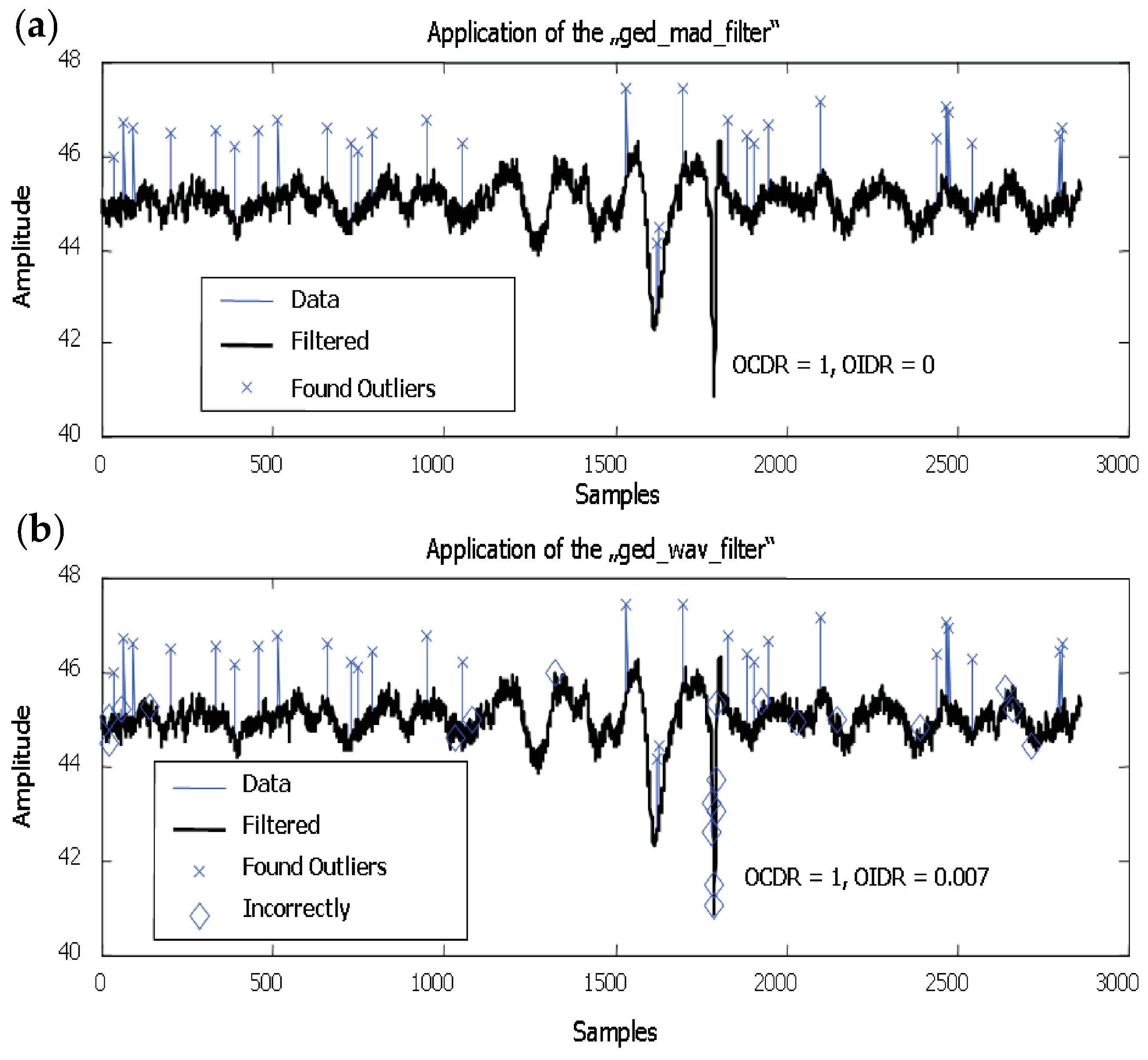
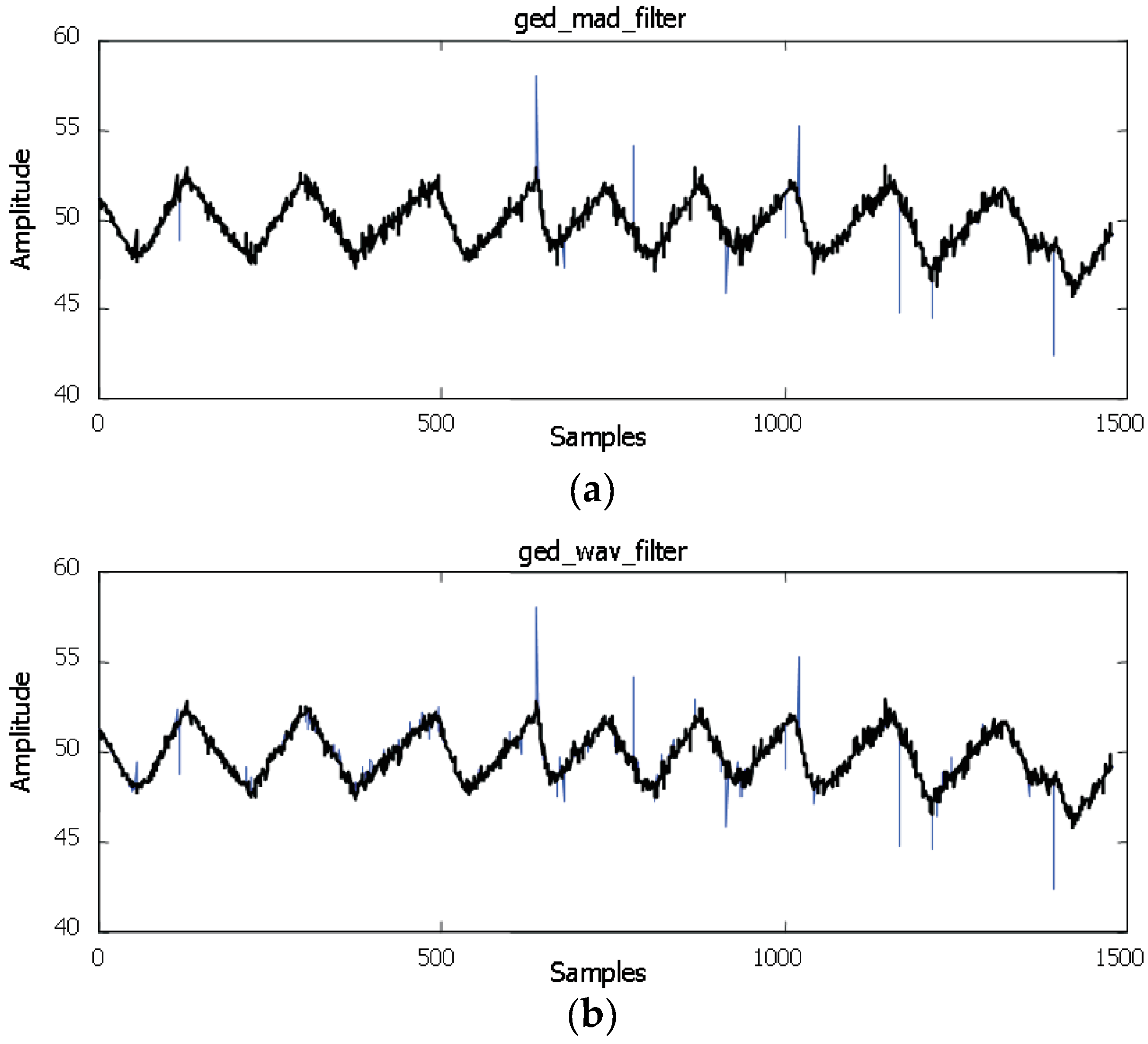
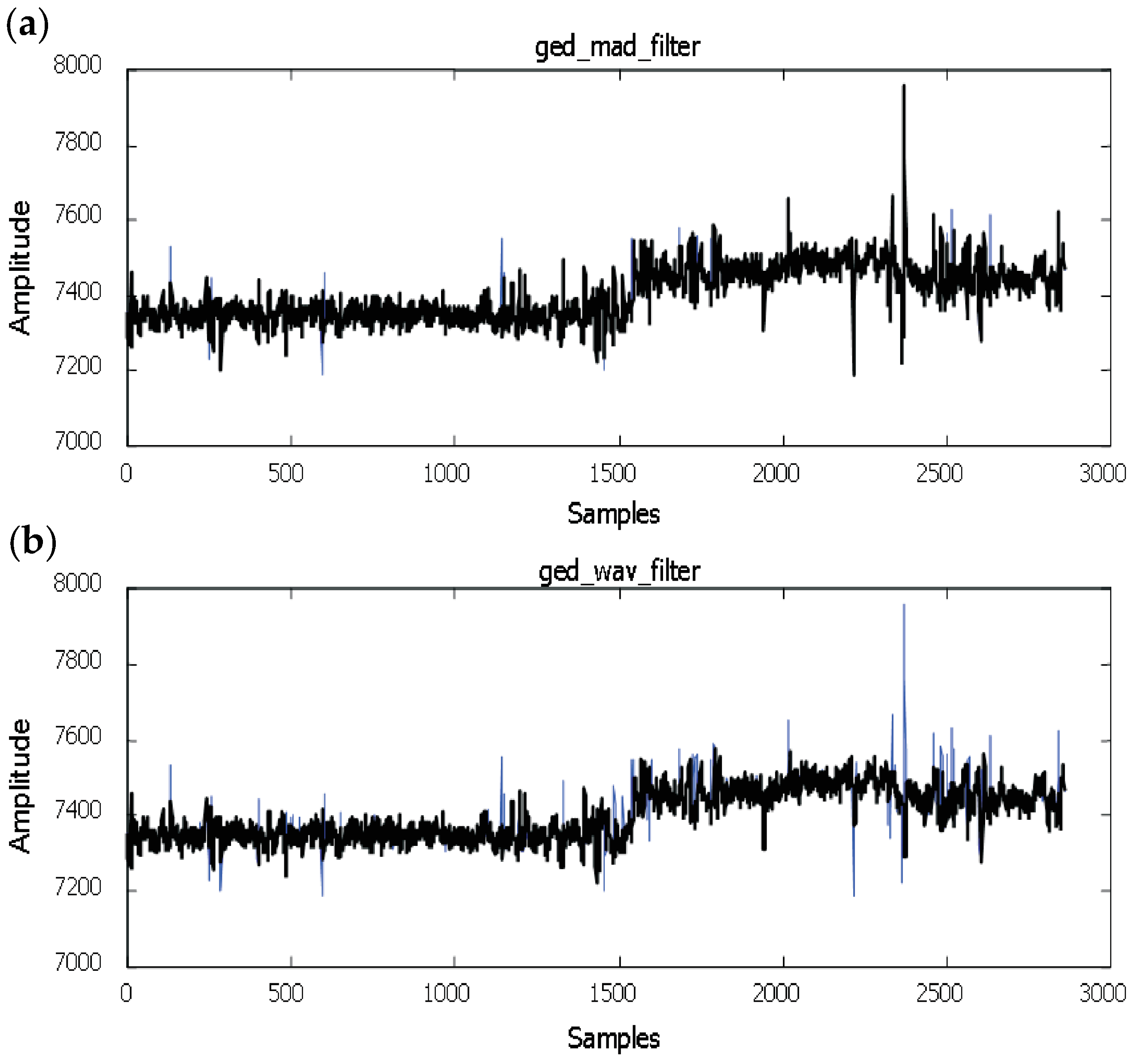
As already mentioned, the developed algorithm is currently integrated into the inferential modelling platform of the unit responsible for Advanced Control and Simulation Solutions within ABB’s (Asea Brown Boveri) industry division. Experimental results using sensor measurements of temperature, and pressure in a Distillation Column are presented in this session. In particular, a process is taken into consideration, and this is represented by a dryer section within a paper mill, and it uses steam at different pressures for the drying. The measured quantities are, as already mentioned, temperature, pressures, flow rates, moisture, and levels, and they include process variables, set point variables, manipulated variables, and disturbances. Figure 7 shows the result obtained from the offline mode to validate the presented algorithm. Figure 7a shows data with artificial outliers. In Figure 7b, all of the outliers are correctly detected, and no misclassifications occur using the proposed algorithm with no priori knowledge of the noise. It is possible to notice that almost 100 % of outliers are detected in the data in the right way. The rate of the incorrect outliers detected in the data can be higher in the first part of the classification because of the initialisation part of the algorithm in which a statistic is built using the local Lipschitz approach already discussed. The initial standard deviation of the local Lipschitz constant is very small when the algorithm starts. The starting phase can take some samples, normally 15–20 samples. It is the weak point of the procedure being a stochastic one, and, in some cases, it can be not robust. The most difficult situation is if the standard deviation of the local Lipschitz constant is small. The algorithm considered in [5] and the one presented in this contribution are compared. The upper parts of Figure 8, Figure 9 and Figure 10 show the results using an algorithm developed in [5] (median filter technique) based on an application of the wavelet filter in the distillation column case. They are compared with the proposed algorithm in which they are shown in the lower parts of the same figures. To summarise the results, it is possible to notice that the proposed algorithm with respect to that proposed in [5] results to be “more aggressive” in the sense that, presumably, it eliminates data that does not belong to the fault set. This is due to the fact that, with respect to the algorithm developed in [5], which is based on a median filter technique, this new method is statistically based, and it is sensible for the chosen threshold (soft, hard and very hard threshold).
More in detail, in Figure 8, a data set from the distillation column case has been contaminated with the outliers. As it can be seen, the MAD algorithm performs much better than the wavelet based one. The MAD algorithm removes all of the outliers and does not remove any measurements that are not outliers. On the other hand, the wavelet based approach removes some of the measurement noise and, more seriously, also some of the signals.
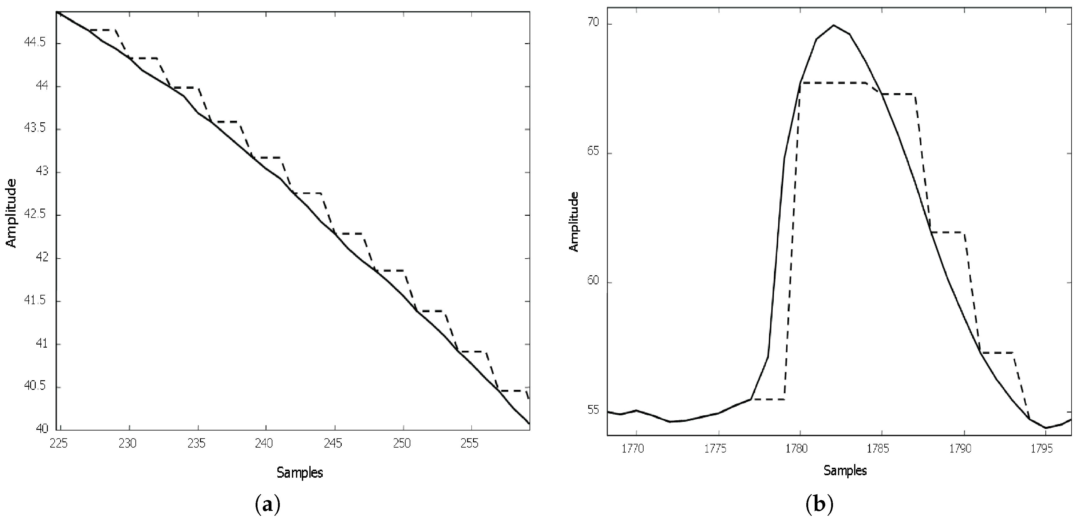
Misclassifications of the outliers can be particularly found in the first part of the data, as it can be seen from Figure 7. The detected rate of the faulty outliers in the data expands in the first part of the classification. The sampling period is usually requested in a linear case to be one-tenth of the "dominating" system time constant. A part of misclassification problems are presented below. It can be clarified by the fact that the chosen sample time of the algorithm is too long if we compare it with the time constant (dynamics) of the considered signal. This algorithm demonstrates other problems, as it can be seen from Figure 11. The algorithm has a problem with following the signal changes when they occur very quickly. In this case, the algorithm can erroneously interpret the changes as sequences of outliers.

6. Conclusions

This work is devoted to the Gross Error Detection applying a wavelet signal based approach. To be more precise, it describes a signal-based algorithm, which can be implemented in industry. This algorithm can be used for solving various problems. Identification of inductance and resistance of an electrical systems is treated in this contribution. A priori knowledge of the noise level is not required for the presented algorithm. Computer simulations and industrial real cases were also treated in this work.

Acknowledgments

The author is grateful to the ABB (Asea Brown Boveri), Ladenburg (Germany) for the technical support of this work. This work could not have been done without their support.

Conflicts of Interest

The author declares no conflict of interest.

References

  1. Albuquerque, J.; Biegler, L. Data reconciliation and gross-error detection for dynamic systems. AIChE J. 1996, 42, 2841–2856. [Google Scholar] [CrossRef]
  2. Coifman, R.; Wickerhauser, M. Entropy based algorithm for best basis selection. IEEE Trans. Inf. Theory 1992, 38, 712–718. [Google Scholar] [CrossRef]
  3. Shao, R.; Jia, F.; Martin, E.; Morris, A. Wavelets and non linear principal component analysis for process monitoring. Control Eng. Pract. 1999, 7, 865–879. [Google Scholar] [CrossRef]
  4. Beheshti, S.; Dahleh, M. On denoising and signal representation. In Proceedings of the 10th Mediterranean Conference on Control and Automation (MED2002), Lisbon, Portugal, 9–12 July 2002.
  5. Menold, P.; Pearson, R.; Allgöwer, F. Online outlier detection and removal. In Proceedings of the 7th Mediterranean Conference on Control and Automation (MED1999), Heifa, Israel, 28–30 June 1999.
  6. Pearson, R. Exploring process data. J. Process Control 2001, 11, 179–194. [Google Scholar] [CrossRef]
  7. Pearson, R. Outliers in process modelling and identification. IEEE Trans. Control Syst. Technol. 2002, 10, 55–63. [Google Scholar] [CrossRef]
  8. Beheshti, S.; Dahleh, M. Noise variance and signal denoising. In Proceedings of the 2003 IEEE International Conference on Acustic Speech, and Signal Processing (ICASSP), Hong Kong, China, 6–10 April 2003; pp. 185–188.
  9. Schimmack, M.; Mc Gaw, D.; Mercorelli, P. Wavelet based Fault Detection and RLS Parameter Estimation of Conductive Fibers with a Simultaneous Estimation of Time-Varying Disturbance. In Proceedings of the 15th IFAC Symposium on Information Control Problems in Manufacturing, INCOM 2015, Ottawa, ON, Canada, 11–13 May 2015; Volume 48, pp. 1773–1778.
  10. Mercorelli, P.; Frick, A. Industrial applications using wavelet packets for gross error detection (Chapter 4). In Computational Intelligence in Information Assurance and Security; Nadjah, A.A.N., Mourelle, L., Eds.; Springer-Verlag: Berlin/Heidelberg, Germany; New York, NY, USA, 2007; pp. 89–127. [Google Scholar]
  11. Mercorelli, P. Using Haar Wavelets for Fault Detection in Technical Processes. In Proceedings of the 13th IFAC and IEEE Conference on Programmable Devices and Embedded Systems, Cracow, Poland, 3–15 May 2015; Volume 48, pp. 37–42.
  12. Donoho, D.L. Denoising by soft thresholding. IEEE Trans. Inf. Theory 1995, 41, 613–627. [Google Scholar] [CrossRef]
  13. Rakowski, W. Prefiltering in Wavelet Analysis Applying Cubic B-Splines. Int. J. Electron. Telecommun. 2014, 60, 331–340. [Google Scholar]
  14. Frick, A.; Mercorelli, P. Spurious Measurement Value Detection Method Uses Wavelet Functions in Defining a Reporting Window for Rejecting Spurious Values in a Continuous Digital Sequence of Measurement Values. DE Patent 10225343 (A1), 18 December 2003. (In German)[Google Scholar]
  15. Donoho, D.L. Denoising and soft Thresholding. IEEE Trans. Inf. Theory 1995, 41, 613–627. [Google Scholar] [CrossRef]
  16. Donoho, D.L.; Johnstone, I.M.; Kerkyacharian, G.; Picard, D. Density estimation by wavelet thesholding. Ann. Stat. 1996, 24, 508–539. [Google Scholar]
  17. Mercorelli, P. A Wavelet Based Algorithm without a Priori Knowledge of Noise Level for Gross Errors Detection. In Advances in Intelligent Systems Research; Atlantis Press: Amsterdam The Netherlands, 2015; ISBN 978-94-6252-000-4. ISSN: 1951–6851. [Google Scholar]
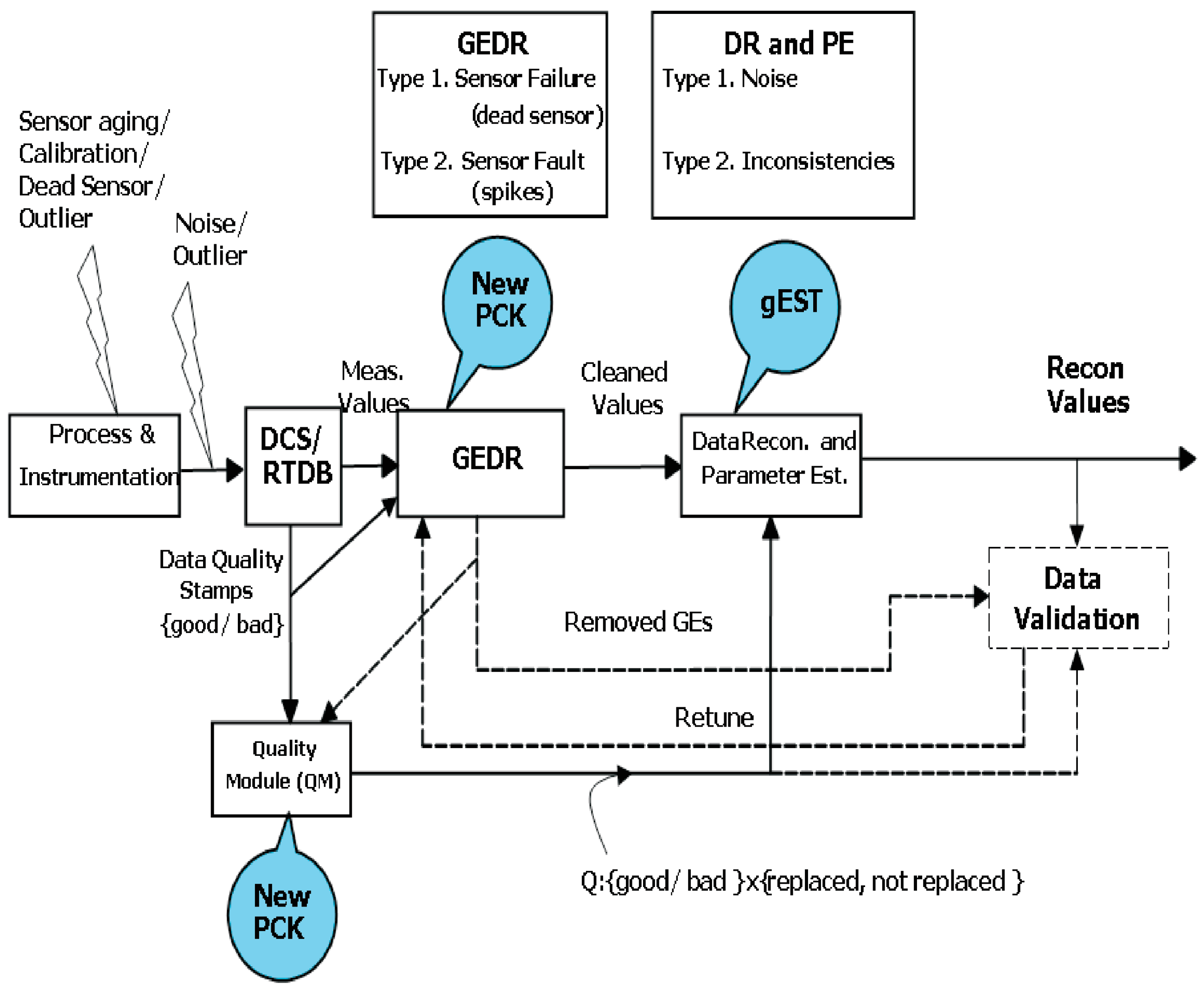
Figure 1. Overview of modules relevant to gross error detection and replacement (GEDR) and quality module (QM).
Algorithms 10 00013 g001
Figure 2. Example of contaminated temperature measurements. With outliers (top) and minimum, maximum limits. The clean temperature data is obtained with help of GEDR.
Algorithms 10 00013 g002
Figure 3. Application of the wavelet based algorithm applied to the mining data.
Algorithms 10 00013 g003
Figure 4. A set of Haar functions.
Algorithms 10 00013 g004
Figure 5. Wavelet coefficients arranged in a tree.
Algorithms 10 00013 g005
Figure 6. (a) multiple outliers; (b) inverse outliers.
Algorithms 10 00013 g006
Figure 7. Simulations by using wavelet algorithms without a priori knowledge on the noise. (a) data with artificial outliers; (b) outliers correctly detected.
Algorithms 10 00013 g007
Figure 8. Comparison between (a) the presented algorithm in [10] and (b) that wavelet based on [5] proposed here.
Algorithms 10 00013 g008
Figure 9. Comparison between (a) the presented algorithm in [10] and (b) that wavelet based on [5] proposed here.
Algorithms 10 00013 g009
Figure 10. Comparison between (a) the presented algorithm in [10] and (b) that wavelet based on [5] proposed here.
Algorithms 10 00013 g010
Figure 11. Problems for the wavelet approach. (a) case of too long sampling time with respect to the dynamics of the system; (b) signal which changes very quickly.
Algorithms 10 00013 g011