Article

Modeling Landscape Evapotranspiration by Integrating Land Surface Phenology and a Water Balance Algorithm

U.S. Geological Survey (USGS), Earth Resources Observation and Science (EROS) Center, Sioux Falls, South Dakota 57198, USA
Algorithms 2008, 1(2), 52-68; https://doi.org/10.3390/a1020052
Submission received: 19 September 2008 / Accepted: 23 October 2008 / Published: 30 October 2008
(This article belongs to the Special Issue Sensor Algorithms)

Abstract

:
The main objective of this study is to present an improved modeling technique called Vegetation ET (VegET) that integrates commonly used water balance algorithms with remotely sensed Land Surface Phenology (LSP) parameter to conduct operational vegetation water balance modeling of rainfed systems at the LSP’s spatial scale using readily available global data sets. Evaluation of the VegET model was conducted using Flux Tower data and two-year simulation for the conterminous US. The VegET model is capable of estimating actual evapotranspiration (ETa) of rainfed crops and other vegetation types at the spatial resolution of the LSP on a daily basis, replacing the need to estimate crop- and region-specific crop coefficients.

Graphical Abstract

1. Introduction

Evapotranspiration (ET) is an important component of the hydrologic budget because it expresses the exchange of mass and energy between the soil-water-vegetation system and the atmosphere. The prevailing weather conditions influence the potential, or reference, ET through variables such as radiation, temperature, wind, and relativity humidity. In addition to these weather variables, actual ET (ETa) is also affected by land cover type, land cover condition, and soil moisture. ETa’s dependence on land cover and soil moisture, along with its direct relationship with carbon dioxide assimilation in plants, makes it an important variable to monitor and estimate crop yield and biomass for decision makers interested in food security, grain markets, water allocation, and carbon sequestration.
Although the estimation of ETa is the ultimate goal of many researchers for hydrological and agronomical applications, it is often difficult to quantify and requires expensive instrumentation. However, different hydrological modeling techniques are used to estimate ETa. The two broad modeling techniques can be grouped as either based on surface energy balance (e.g., [1]; [2]; [3]; [4]; [5]) or water balance principles (e.g., [6]; [7]; [8]). More recently, Wang et al. [9] developed a regression equation to estimate ETa from a combination of net radiation, vegetation index, and temperature.
The choice of the model type depends on the availability of data and on the objective of the project. For example, the presence of cloud cover adversely impacts the surface energy balance models, but it does not impact the water balance model, which explicitly takes cloud information into consideration in the satellite-based rainfall estimation process. This feature guarantees a reliable daily ETa estimation in much of the rainfed vegetation systems regardless of cloud cover. This can be a significant advantage during the growing season in many parts of the world. On the other hand, the surface energy balance model has the advantage of estimating “total” ET irrespective of the water source, whereas the water balance model only estimates “rainfed” ET. This difference creates the opportunity to identify landscapes that meet their ET from external (e.g., stream diversion) or groundwater sources. In this study, a landscape is defined as the modeling spatial unit as determined by the resolution of the Land Surface Phenology (LSP).
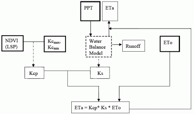
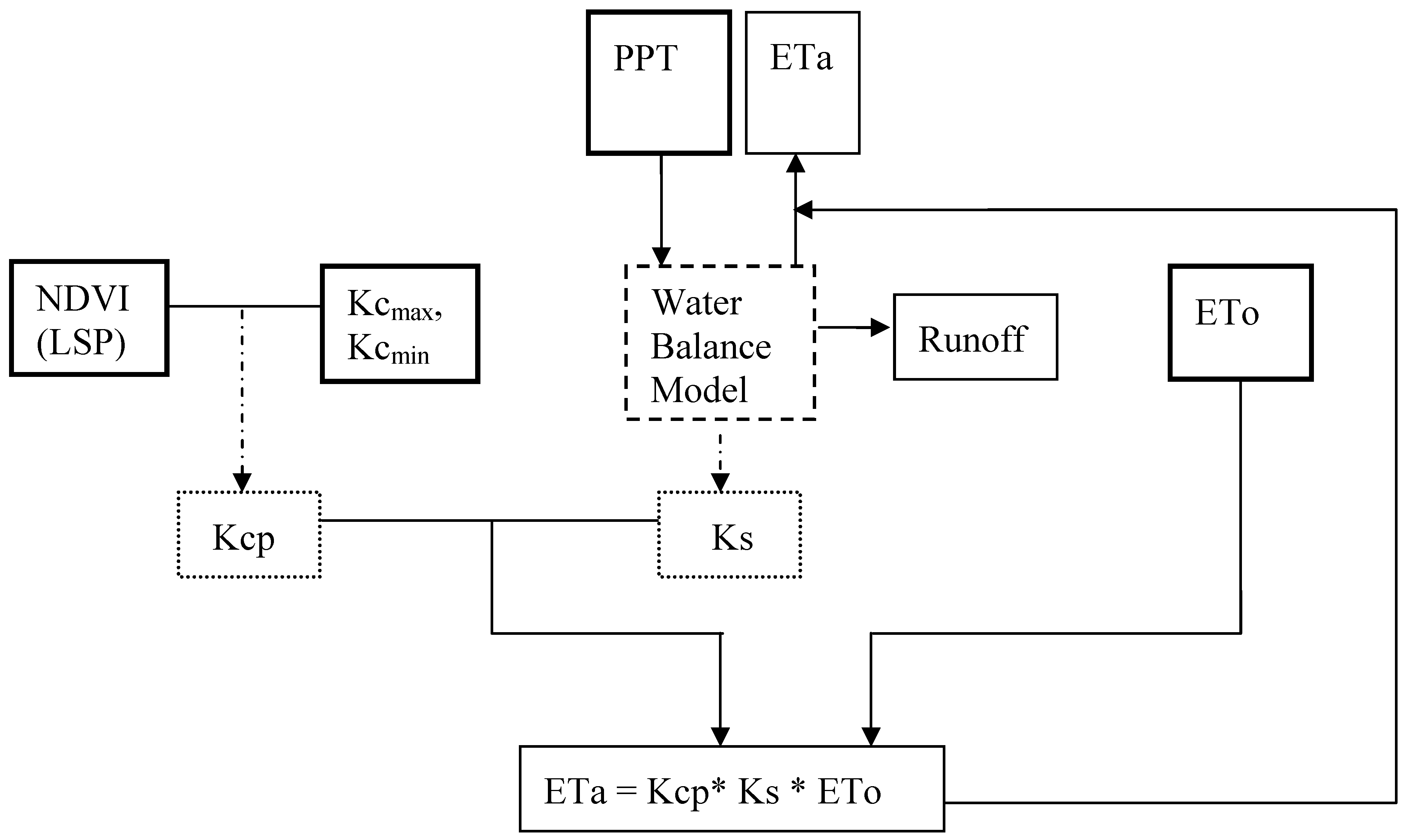
The main objective of this study is to present an improved modeling technique called Vegetation ET (VegET) that integrates commonly used water balance algorithms with remotely-sensed LSP-parameter (Figure 1) to conduct operational vegetation water balance modeling at the spatial resolution of the LSP data set using readily available global data sets.

Background

The most widely used crop water balance technique for operational monitoring is the Food and Agriculture Organization (FAO) water balance algorithm by Doorenbos and Kassam [10] that produces the crop water requirement satisfaction index (WRSI). The WRSI shows the relative relationship (ratio/percent) between the supply (from rainfall and existing soil moisture) and demand (crop demand to meet its physiological needs) using observed data from the beginning of the crop season (planting) until a specified date throughout the growing season.
The Famine Early Warning System Network (FEWS NET) demonstrated a regional implementation of the FAO WRSI in a grid-cell modeling environment [7]. Furthermore, Senay and Verdin [8] enhanced the geospatial model by introducing the concept of maximum allowable depletion (MAD) and soil water stress factor, commonly used in irrigation engineering, for better estimation of ETa as a function of soil water content in an operational setup (http://earlywarning.usgs.gov/adds/). The WRSI crop water balance index has been demonstrated to be a reliable tool for crop performance monitoring of large areas in an operational manner.
However, the use of crop coefficients (Kc) in the model has certain limitations: 1) Kc factors are crop specific and require a prior knowledge of the crop planted in the area, 2) Kc factors are spatially specific since they are influenced by local climate, soils, and other geophysical conditions, and 3) the use of the Kc model requires knowledge (or assumption) of the crop calendar such as the start of season (SOS) and length of growing period (EOS) in each of the four crop developmental stages (initial, vegetative, mature, and senescence).
The VegET modeling approach presented in this paper removes the above constraints by the inclusion of the LSP parameter, which describes the seasonal progression of vegetation growth and development. LSP can be observed by spaceborne sensors and is a key biogeophysical parameter that links the water and carbon cycles with anthropogenic activities, providing an important approach to change detection in terrestrial ecosystems (e.g., [11]; [12]; [13]; [14]).
This paper will discuss the formulation of the LSP-based Kc parameter function in the VegET model and demonstrate its application using two years of daily meteorological data in the conterminous United States. To differentiate the LSP-based Kc from the commonly used “crop coefficient,” the designation Kcp (the “p” denoting the phenology-based coefficient) is used in this study.

2. Materials and Methods

2.1 Study Area and Data

The model development was conducted using data from the conterminous United States because of the availability of field data sets for the validation of some of the model results.
The most important data sets in this study are the Advanced Very High Resolution Radiometer (AVHRR) Normalized Difference Vegetation Index (NDVI) data sets, gridded rainfall, reference ET (ETo), and gridded soil water holding capacity (WHC). In addition, latent heat flux data from AmeriFlux towers were used to validate the results. The average weekly maximum NDVI values (1989–2004) were acquired from the U.S. Geological Survey (USGS) Earth Resources Observation and Science Center (EROS) [15].
Precipitation is a key driver of the water balance model. Daily gridded rainfall data at 5-km spatial resolution was acquired from the National Weather Service (NWS) for 2005 and 2006. The NWS precipitation data is produced as a merged product between WSR-88D NEXRAD (Next Generation Radar) and ground rainfall gauge reports (http://www.srh.noaa.gov/rfcshare/precip_about.php). WHC, in mm per meter depth of soil, is derived from the State Soil Geographic Database (STATSGO) (http://www.ncgc.nrcs.usda.gov/products/data sets/statsgo/) for the United States. Daily ETo is produced at USGS/EROS from 6-hourly meteorological data from the Global Data Assimilation System (GDAS) using the standardized Penman-Monteith equation [2] for the globe [16]. The ETo was scaled down from 1.0 degree to 0.1 degree using the method described in Senay et al. [4]. Model validation data sets on latent heat flux and point-rainfall were downloaded from the AmeriFlux towers sites (http://public.ornl.gov/ameriflux/index.html). Latent heat flux from the AmeriFlux towers is measured using an eddy correlation method. Daily raw 30-minute latent heat flux data (w/m2) downloaded from the Web site were converted into daily ET equivalents using the latent heat of vaporization of water at 2.45 MJ/kg, which is equivalent to using 2.45 MJ of energy to evaporate 0.001 m3 of water (1 mm over 1 m2, assuming 1000 kg/m3 for the density of water). Thus, 1 mm/day of ETa requires an average of 28.356 (2.45 * 106 / (24 * 3600)) w/m2 of power throughout the day. Thus, daily average latent heat flux data in w/m2 from the AmeriFlux towers were converted to ETa equivalents in mm/day using a conversion factor of 0.03525 (1/28.356). In addition, the Moderate Resolution Imaging Spectroradiometer (MODIS) Vegetation Continuous Field (VCF) data was used as an exploratory data set for evaluating the percent vegetation cover in each pixel [17].

2.2 NDVI Climatology vs LSP

The NDVI climatology is defined as a “historical” average NDVI for a given time period. Historical is defined as the average of at least 5 years of NDVI data. Such data is available from AVHRR and MODIS for global applications. In this study, LSPs are simply represented by temporally smoothed (3-period moving average) climatology NDVI data sets. Smoothed NDVI climatology data sets are preferred to produce Kcp functions in order to avoid data noise from yearly NDVI data sets. Currently, NDVI climatology is available for global applications from different data sources such as the Global Inventory Monitoring and Modeling Studies (GIMMS) at a monthly scale at 8-km resolution. In this study, the U.S. weekly maximum composite at 1 km is used [15]. This data set is created by first compositing cloud-free weekly maximum NDVI values for each pixel from 1989 to 2004. The climatology was then created by averaging weekly maximum NDVI values over the 16 years. The weekly climatology NDVI were further interpolated to represent dekadal time periods to conform with other modeling procedures and availability of similar (dekadal) NDVI data sets for other regions of the world. A dekad is nominally composed of 10-day time periods in a month, except for the 3rd dekad of a month where it may assume values of either 8, 9, 10, or 11, depending on the month and year. Depending on the context of the discussion, the terms LSP and NDVI climatology are used interchangeably.

2.3 Crop Coefficient (Kc)

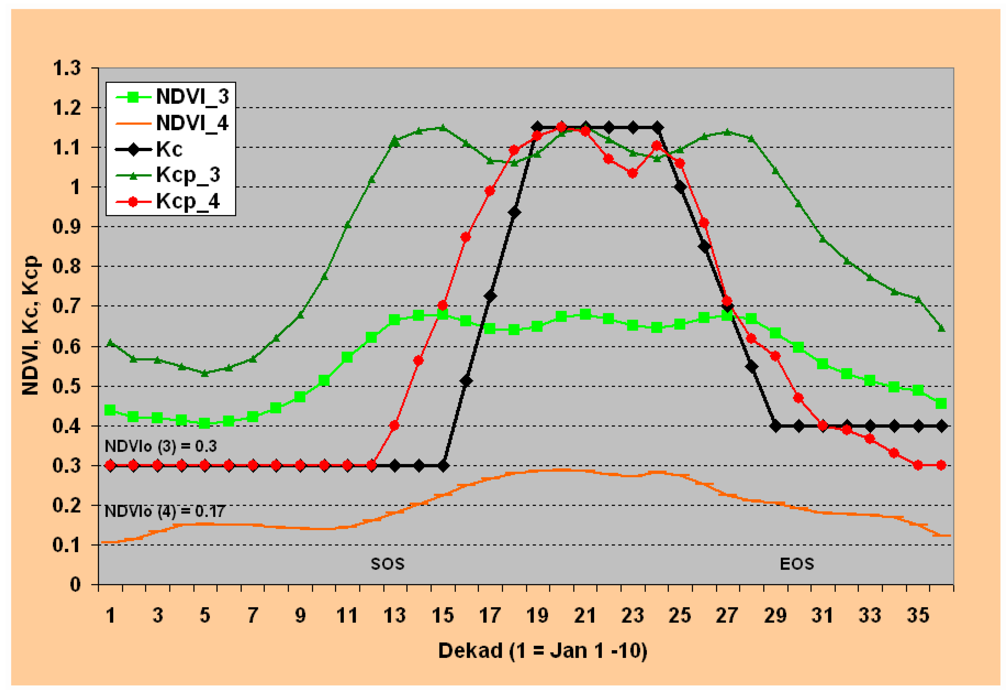
To compare the differences between a generic cereal crop Kc and the spatially dynamic Kcp, a crop coefficient function was developed using the following assumptions. The study assumes a generic cereal crop with a growing length of 170 days. The growing lengths for the initial, vegetative, mature, and senescence growing stages are 30, 40, 50, and 50 days, respectively. The associated Kc values for the initial, mature, and senescence periods are 0.3, 1.15, and 0.4, respectively [6]. The temporal plot of the Kc function is shown in Figure 2 and Figure 3 along with the corresponding Kcp functions. Although the evaluation is shown for generic cereal crops as an example, the procedure is applicable for other crops or vegetation types.

2.4 Model Formulation

2.4.1 Basic Model Setup

VegET monitors soil water levels in the root zone through a daily (or longer time step) water balance algorithm to estimate ETa in rainfed landscapes. The key input data to VegET are precipitation (PPT), ETo, WHC, and Kcp. ETa is calculated as the product of ETo, soil stress coefficient (Ks), and Kcp, as shown in Equation 1. Figure 1 shows a simplified schematic representation of the VegET model.
E T a = K c p K s * E T o
Where ETa is actual evapotranspiration in mm; Kcp is LSP-derived crop coefficient (-); Ks is soil-water stress coefficient (-) and ETo is reference ET in mm.
Ks is determined from a soil water balance model similar to the one developed by Senay and Verdin [8] for USGS/FEWS NET early warning applications using Equation 2. The dimensionless Ks coefficient varies from 0.0 to 1.0 depending on the soil water level in the modeling unit root zone.
K s = S W i M A D S W i < M A D ; K s = 1.0 S W i > = M A D
SWi is soil water of current time step in depth unit. MAD is the Maximum Allowable Depletion level of soil water in the root zone, below which the vegetation ET is less than “potential” and will be constrained by the availability of soil water according to Equations 3. Although MAD varies by crop/vegetation type, a nominal value of 50% of the soil WHC can be used for most generalized crops such as cereals and natural vegetation. Thus, MAD was estimated as 50% of the WHC derived from STATSGO.
The soil water level is determined using a daily soil water balance using Equation 3 where ETa is estimated iteratively employing Equations 1 and 2. The model estimates a combined runoff and deep drainage based on the principle of saturation excess where soil water in excess of the water holding capacity (WHC) of the soil is considered to be unavailable for plant–use in the root zone; thus SWi is set to a maximum of WHC and a minimum of 0.0 during the modeling time-step. More detailed information is available on the setup and initialization of the soil water balance model for operational crop monitoring in Senay and Verdin [8].
S W i = S W i 1 + P P T i E T a i
Where SWi is soil water of current time step (mm); SWi-1 is soil water of the previous time step (mm); PPTi is precipitation (mm) and ETai is actual ET (mm); “i” is the modeling time step.
The innovative approach in VegET is on the calculation of the Kcp (Figure 1). The Kcp is comparable to the Kc widely used by agronomists [6]. The key difference is that Kcp is a parameter derived from remotely sensed data as opposed to site-specific field experiments. Kcp represents both the spatial and temporal dynamics of the landscape water-use patterns on a grid-cell basis. LSPs are characterized and converted into Kcp parameter functions for each modeling grid cell using LSPs generated from NDVI climatology.

2.4.2 Justification for Introducing Kcp

In this formulation, the Kcp parameter will replace the Kc that has been widely used for crop water balance studies around the world to simulate crop water-use patterns during a crop growing season. Researchers have shown that NDVI is linearly related to Kc ([18]; [19]; [20]; [21]). Bausch [22]demonstrated the use of the soil adjusted vegetation index (SAVI) to extrapolate Kc for corn throughout the growing season. In this study, a simple linear relationship is formulated to convert LSPs into water-use patterns for operational applications. The designation Kcp (the “p” denoting the phenology-based coefficient) is used to distinguish it from the Kc that is derived from experimental plots in the FAO method [6].
Figure 1. A simplified conceptual diagram of the VegET model. Major inputs are: precipitation (PPT), reference ET (ETo) and NDVI/Kc. Estimated parameters are phenology-based crop coefficient (Kcp) and soil-water stress factor (Ks). Model outputs are ETa and runoff.
Algorithms 01 00052 g001
Since Kc is a step-function, the following assumptions and simplifications have been introduced to simulate the Kc water-use patterns from LSP profiles. The Kc function is based on four growth stages of the vegetation: early, vegetative, maturity, and senescence. The early and mature stages are constant functions of time, while the vegetative (increasing) and senescence (decreasing) stages are linear functions of time.
Similarly, the Kcp function is developed by assuming a constant water-use pattern in the early and late stages when the LSP value falls below a certain threshold. On the other hand, Kcp values between the initial and mature stages will vary according to the NDVI (LSP) profile, while the Kc values are derived as a linear function of time. The challenge has been the establishment of the threshold values that signal the start of a season that marks the end of the initial period. Although this model parameter can be adjusted to reflect regional or sensor conditions, a trial-and-error method was used to assign the initialization threshold to an NDVI value of 0.30 when using NDVI derived from AVHRR data sets. Although this threshold is appropriate for a large area of the Earth where there is reasonable vegetation cover for parts of the year, the threshold is dynamically adjusted to handle landscapes in mainly arid and some semiarid regions with little or no vegetation cover.
The Kcp parameter has major advantages over the predecessor Kc. Since Kcp is derived from LSPs that are unique to each modeling cell in the world, there is no need to redefine Kcp by region and climate as is the case for Kc. Kcp includes the vegetation calendar, i.e., start of season, length of growing period, and end of season from the LSP. By contrast, crop-specific growth stage, timing, and length have to be assumed in the case of Kc. Because of the embedded vegetation calendar in LSPs, vegetation water balance studies can be initiated without the need to assume or model separately the start of the growing season for operational vegetation and crop monitoring.

2.4.3 Kcp Parameter Function

The Kcp parameter function is defined using NDVI climatology (LSP) and published crop coefficient minimum (Kcmin) and maximum (Kcmax) values. The Kc values provide the lower and maximum limits for the Kcp. The NDVI profile provides the temporal patterns of Kcp. Kcmax and Kcmin values can be defined under two conditions: 1) with the assumption that a specific crop/vegetation type will grow in a modeling cell (in this case, published values from FAO [6] or other sources can be used), 2) with the assumption that the landscape ET is based on different land cover mixtures as captured by the NDVI profile; i.e., a modeling cell will include fractions of different vegetation types and bare cover. In the second case, Kcmax and Kcmin can be a composite value from a weighted average of the cover composition with each modeling cell. The percent cover fractions from the MODIS VCF data will be particularly useful for this application.
Equation 4 shows the formulation of the Kcp parameter as used in Equation 1 to estimate landscape ET, representing a spatial unit as determined by the resolution of the LSP data set (NDVI).
K c p = K c max K c min N D V I max N D V I o ( N D V I i N D V I o ) + K c min
K c p = K c min K c p < K c min
Where Kcmax is the maximum (mature) Kc value for a vegetation/crop type; Kcmin is the minimum (early stage) Kc value; NDVImax is the climatology maximum NDVI value in a year; NDVIi is the climatology NDVI value for a given period “i” (average weekly maximum value in this case); and NDVIo is the minimum reference NDVI value that is associated with the minimum Kc value, which varies depending on the value-range of NDVImax according to Equation 6 or 7.
NDVIo is calculated depending on the NDVImax for each pixel.
CASE 1: NDVImax > = 0.40
N D V I o = 0.3
CASE II: NDVImax < 0.40
N D V I o = 0.33 ( N D V I max N D V I min ) + N D V I min
NDVImin is the climatology minimum NDVI value from the weekly maximum NDVI composite data set.
The justification for establishing the NDVIo value is based on observations of the start of season in crop and grassland phenology. A value of close to 0.3 AVHRR NDVI generally corresponds to the start of the green-up period. This is generally true for areas with crop and grassland systems where the fraction of the vegetation coverage is relatively high. However, in sparsely vegetated areas the magnitude of the NDVI is so low that even the maximum NDVI is sometimes less than the minimum threshold level of 0.3 that is considered an indication of the start of season in predominantly cropland areas (Figure 2 and Figure 3). To better handle sparsely vegetated areas, the NDVIo value is defined in relation to the maximum NDVI value for such regions. By visual inspection of several LSP profiles, pixels with NDVI maximum values less than 0.4 are considered sparsely vegetated. For the conterminous United States, only 18.6% of the area had an NDVImax value lower than 0.4. These areas were mainly concentrated in the arid and semiarid southwest.
For arid pixels, the NDVIo parameter will be calculated dynamically, as shown in Equation 7. The most useful information required is the timing and relative magnitude of water use. Although we move the NDVIo threshold value from 0.3 to some lower number, the timing and relative magnitude of water use will still be achieved (Figure 2 and Figure 3). This is possible because the absolute NDVI magnitude of a pixel is a function of the percent vegetation cover, but the phenology (timing and relative magnitude of water use) is mainly captured by the temporal profile of the NDVI pattern.
Assigning a Kcmax value for Kcp during the peak NDVI is only appropriate if the objective is to simulate crop water use by assuming the entire modeling unit is composed of crop fields. Because crop growers make sure there is good ground coverage (closed canopy) at maturity for most crops, the Kcp function assumes that maximum water use is achieved at maximum NDVI regardless of the magnitude of the maximum NDVI. The NDVI profile provides the timing and relative magnitude of water use. On the other hand, if the exercise is to simulate landscape water use by the natural vegetation, the maximum and minimum Kc (Kcmax, Kcmin) can be adjusted as an area-weighted value to reflect this based on information on percent ground cover from such data sources as MODIS VCF.
A justification of the 0.33 coefficient in Equation 7 is derived from the observation that 0.3 NDVIo value for crop/grassland areas also corresponds to approximately one-third plus the minimum NDVI of the range between the maximum NDVI (0.7) and minimum NDVI (0.1) generally found in crop and grassland systems (0.2 + 0.1). Thus, with a similar logic, the NDVIo for vegetation sparse regions is defined using Equation 7. These thresholds have been shown to produce reasonable results for the United States. However, sensor-specific adjustments may be necessary when using NDVI data sets from sources other than the AVHRR climatology. The main impact of the lower or higher NDVIo value is in the starting of vegetation growth simulation to the earlier or later part of the season, respectively. For example, a change from NDVIo of 0.25 to 0.3 may move the start of season by two weeks later. This kind of error is tolerable when the main objective is to monitor the performance of crops or vegetation at large spatial (> 5 km) and temporal (> monthly) time scales. This error is even more tolerable when the seasonal monitoring is compared with other years as an anomaly product.
The Kcp function only uses these two parameters (NDVImax and NDVIo) to convert smoothed historical NDVI data sets from NDVI to Kcp according to Equation 4 or 5. For example, a generic cereal crop has a published Kc of 0.3 (Kcmin) at the early stage and 1.15 (Kcmax) for the mature stage. Both NDVImax and NDVImin (NDVIo) are calculated from NDVIi data sets where “i” represents a “historical” NDVI time step. NDVIi data sets are available at weekly or longer time steps.

2.5 Analysis Procedure

To demonstrate the applicability of the modeling algorithm under different land cover conditions, four separate locations with different climate and land cover composition were chosen in the United States. The selection was conducted deliberately through a trial-and-error method until NDVI profiles representing grassland, crop, and forest areas were found (Figure 2). The locations of the four study sites are shown in Figure 4a and Figure 4b. The location identifiers are labeled based on the bare percent from the MODIS VCF data set. Therefore, identification marks (IDs) with B0, B1, B21, and B42 labels represent bare percentage of 0.0% in a single pixel in Virginia, 1% in Illinois, 21% in North Dakota, and 42% in Wyoming, respectively. The respective geographic coordinates (lon/lat) for the study sites are: -79.85, 36.92; -89.05, 41.93; -103.35, 48.82; -108.55, 44.82. In addition to the four sites where NDVI profiles have been converted to Kcp parameter functions (Figure 3), two additional sites in Brookings, South Dakota (lon/lat: -96.84, 44.35), and Audubon, Arizona (lon/lat: -110.51, 31.59), were used to validate daily ETa modeling results using AmeriFlux latent heat flux data (Figure 4 and Figure 5). These sites were chosen because of the availability of near-complete data sets (less than 12 days missing) for the entire year in 2005 and their contrast in vegetation dynamics. The contrast between the two sites can be characterized by the differences in maximum and minimum NDVI climatology. The Arizona site has an NDVI climatology range between 0.20 and 0.44, while the corresponding values for the South Dakota site are 0.18 and 0.69.
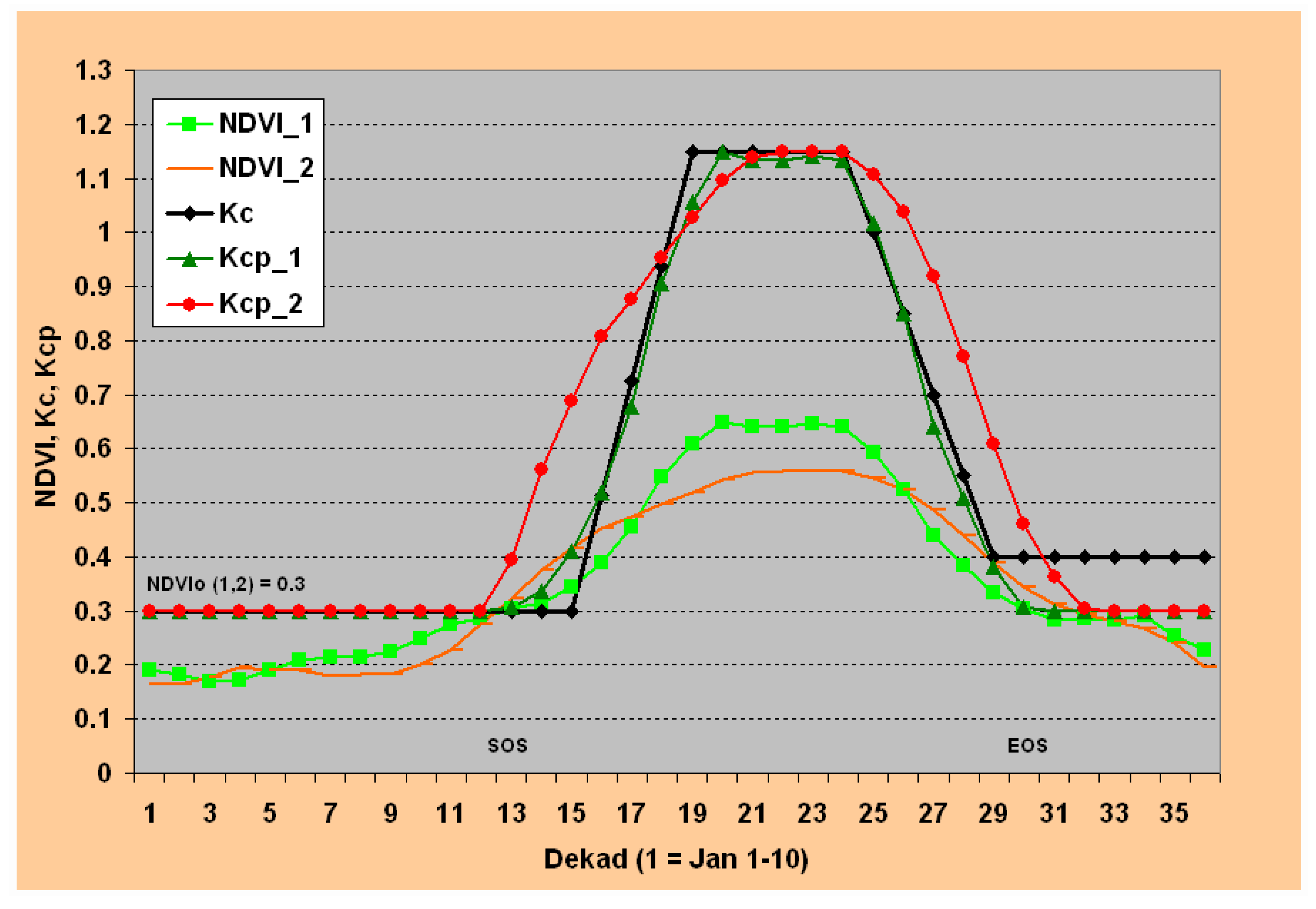
Figure 2. Temporal profile of AVHRR NDVI climatology, corresponding Kcp, and control Kc profiles for two potential cropland locations with different proportion of bare (B), herbaceous (H), and tree (T) cover percentages. NDVI_1: B = 1%, H = 72%, T = 27%; NDVI_2: B = 21%, H=77%, T=2%.
Algorithms 01 00052 g002
Figure 3. Temporal profile of AVHRR NDVI climatology, corresponding Kcp, and control Kc profiles for two noncropland locations with different proportion of bare (B), herbaceous (H), and tree (T) cover percentages. NDVI_3: B = 0%, H = 62%, T = 38; NDVI_4: B = 42%, H= 58%, T=0%.
Algorithms 01 00052 g003
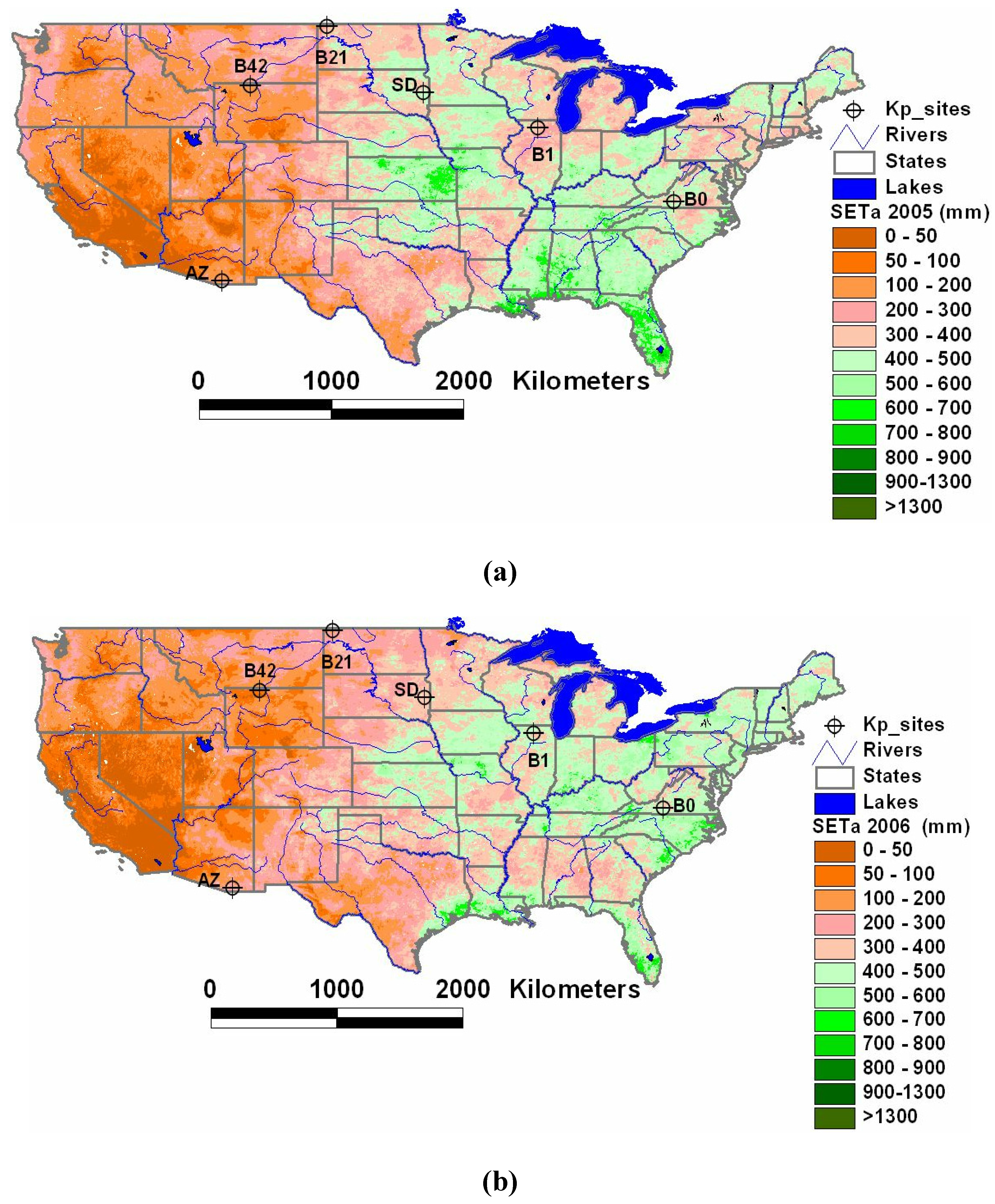
The VegET model was run using two years of daily meteorological data from 1 January to 31 December for 2005 and 2006. In order to reduce computational burden, the spatial resolution of the rainfall (5 km) was chosen instead of the LSP (1-km) for the conterminous US. Daily ETa estimates were extracted to compare with two AmeriFlux latent heat flux data sets for 2005. Seasonal ETa totals were made by summing up daily grids from 1 May to 30 September for both years to show the spatial distribution of seasonal ETa in a given year and change on a pixel-by-pixel basis between 2005 and 2006.

3. Results and Discussion

Figure 2 shows the temporal plots of dekadal NDVI climatology and the corresponding Kcp and Kc for two locations with a high proportion of herbaceous cover (potential crop pixels). The major difference between NDVI_1 and NDVI_2 profiles is that NDVI_1 contains a higher proportion of tree (T) cover (27%) and lower bare (B) cover (1%), while NDVI_2 contains a higher proportion of bare (21%) and lower tree (2%) covers. The herbaceous (H) component is comparable on both: 72% and 77% for NDVI_1 and NDVI_2, respectively. Also, NDVI_1 is located in northern Illinois with a “B1” marker, while NDVI_2 is located in northwestern North Dakota (“B21”) (Figure 4). The numbers in the location marker such as “B1” and “B21” refer to the bare cover percentages. Both locations showed a comparable start of season by crossing the 0.3 NDVI threshold around dekad 12 (20–30 April). The overall seasonal pattern is comparable in that both experience their peak NDVI in the time period between dekad 19 and dekad 23. However, NDVI_1 shows a higher magnitude during the peak season while NDVI_2 shows a higher magnitude during the early and late season. Also, NDVI_1 crosses back the 0.3 NDVI threshold about 2 dekads earlier than NDVI_2 toward the end of season.
The corresponding Kcp patterns for NDVI_1 and NDVI_2 are shown as Kcp_1 and Kcp_2. The transformation of NDVI into Kcp patterns involves changes both in magnitude and temporal patterns. For example, in terms of peak magnitude, NDVI_1 is higher than NDVI_2. But the peak magnitude is about the same for Kcp_1 and Kcp_2 mostly because the assumption of cereal crops being grown on both locations with comparable ground cover will result in a comparable peak water-use coefficient under unlimited soil water condition. Temporally, the differences between NDVI and Kcp patterns are more pronounced during early and late seasons. On the other hand, during the dormant stages of the crops (before start of season and after end of season), the Kcp values are held constant to a minimum threshold value of 0.3. The NDVI patterns of the two locations are also close to each other during this period, unlike the peak season. From Figure 2 it can be shown that NDVI_1 will be transformed into a crop water-use pattern (Kcp_1) characterized by a steep increase and decrease in water-use before and after the peak-season, respectively. On the other hand, NDVI_2 will be transformed into a water-use pattern (Kcp_2) characterized by a longer season with a gradual increase and decrease in water use before and after the peak growing season. The actual water use in each case will depend on the atmospheric demand (reference ET) and availability of soil moisture in the area, as shown in Equation 1.
A plot of a typical Kc profile for a cereal crop with a 170-day growing season shows that Kcp_1 closely matches with the Kc curve, indicating that the use of published Kc values will work well for this location. However, the use of a published Kc profile will not represent well the Kcp_2, which will potentially underestimate the overall vegetation water use in this example.
Figure 3 shows the temporal plots of dekadal NDVI climatology and the corresponding Kcp for two other locations with a relatively high proportion of tree cover (0%, 62%, 38% for bare (B), herbaceous (H), and tree (T), respectively) for NDVI_3 and a high proportion of bare areas (42%, 58%, 0% for B, H, T covers, respectively) for NDVI_4. The conversion from NDVI LSP to Kcp has a different effect on the two cover types, especially when compared to the traditional Kc-based water-use pattern. While the temporal pattern of the Kcp_4 (high bare cover) area closely follows the Kc pattern, the Kcp_4 (high tree cover) resembles that of the corresponding NDVI, except for the magnitude. Note that Kcp_4 is generated using Equation 7 to calculate the threshold NDVIo of 0.17, while Kcp_3 used the same NDVIo of 0.3 as in the case of Kcp_1 and Kcp_2 in Figure 2. The main reason for this difference is that the maximum NDVI for NDVI_4 is less than 0.4, triggering the use of Equation 7 to estimate NDVIo. The cutoff value of 0.4 is established arbitrarily from visual inspection of several plots to handle sparsely vegetated areas. The peak NDVI is used as a measure of vegetation density. In this study, the peak NDVI magnitude was strongly correlated (r > 0.89) with the bare area percentage. From the examples of Figure 2 and Figure 3, NDVI_4 has the lowest peak NDVI (< 0.3) with the highest bare percentage (42%), while NDVI_3 has the highest peak NDVI (> 0.65) with a bare percentage of 0.0%.
Figure 4 show the spatial distribution of seasonal (1 May through 30 September) ETa for the generic cereal crops generated using the VegET model for 2005 and 2006, respectively, at 5-km resolution. Generally, it can be observed that the eastern United States has a higher ETa than the western United States in both years, which can be attributed to higher rainfall and vegetation cover. More important for decision makers is that the VegET output shows a gradual subcounty spatial variability and a dramatic year-to-year variability in some places. For example, the 2005 ETa (Figure 4) shows lower ETa (drought) in Illinois, Pennsylvania, and North Carolina with seasonal ETa values as low as 300 mm. By contrast, in 2006, the drought was located in the Dakotas, Oklahoma/Kansas, and Alabama/Georgia. These drought incidences have been reported by various organizations.
For example, Illinois reported the second driest March–August (2005) on record (http://www.ncdc.noaa.gov/oa/climate/research/2005/aug/st011dv00pcp200508.html).
Figure 4. Seasonal VegETa ETa (May–September) maps for 2005 (a) and 2006 (b). Kp_sites refer to locations where the Kcp (B1 – B42) and AmerixFlux (SD, AZ) latent flux data were extracted.
Algorithms 01 00052 g004
Furthermore, preliminary analysis with crop yield data has shown a strong correlation between seasonal ETa and wheat yield in South Dakota, where ETa has explained 60% of the spatial yield variation in 2005 and 2006. The yield decrease from 2005 to 2006 was correctly identified in most counties in South Dakota [23].
It should be pointed out that the relatively low ET in the wet part of the northwest of the US can be explained by two important reasons: 1) the accumulation period for the ET map is between May and September, a generally dry time for the region and 2) the VegET model only monitors rainfed systems and does not take into account snowmelt sources that supply moisture to the natural vegetation and irrigation systems during the dry period. Although the VegET model was run assuming a generic cereal crop over the landscape, the relative ETa spatial distribution will also apply to other natural vegetation types that obtain their water from rainfall since the maximum crop coefficient value for cereal crop and natural vegetation such as grassland is comparable for similar ground cover fraction.
The low ETa for the western part of the United States is mainly a result of the shortage of precipitation and thus the lack of adequate soil water, which affects the Ks factor in Equation 2. From the cereal crop assumption covering the whole modeling unit, these seasonal ETa estimates, despite their low value in the arid and semiarid west, are probably exaggerated on the high side because of the assumption of Kcmax for the entire modeling cell. However, the relative spatial distribution in water use (ETa) is expected to represent the situation in the field as it is demonstrated by flux tower data on two locations with different climate (Figure 5a and Figure 5b).
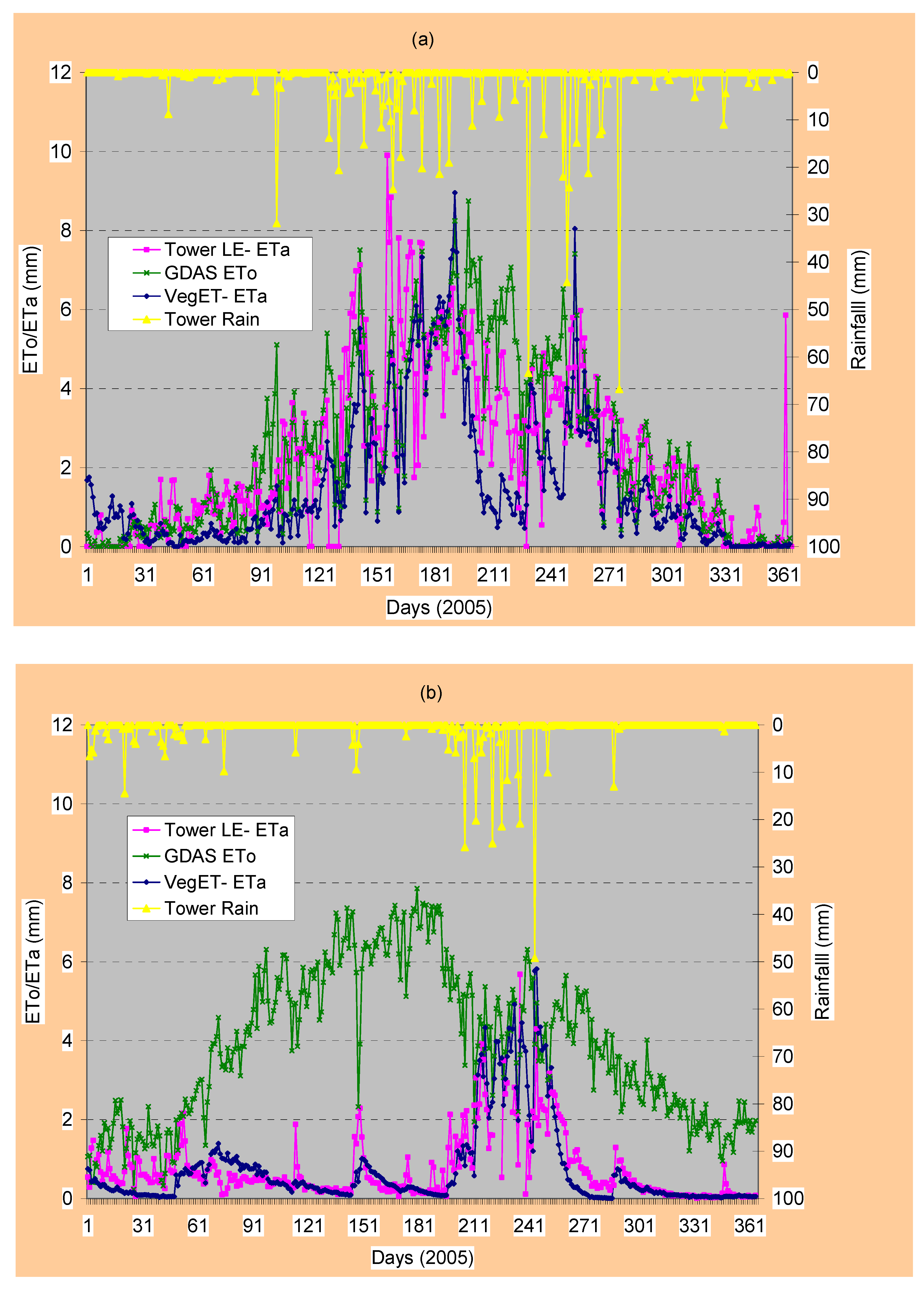
Figure 5a and Figure 5b show a validation of the VegET ETa results using AmeriFlux tower eddy covariance latent heat flux measurements. Figure 5a shows these relationships using flux tower data from Brookings, South Dakota, in a crop/grassland environment, while Figure 5b shows the same relationship in the semiarid grassland of Audubon, Arizona. On both sites, the flux tower latent heat flux ETa and VegET ETa tracked well, capturing the seasonality of ETa with comparable magnitudes. The major difference between the two sites is that the ETa was much lower than the ETo during the dormant vegetation growing season in the Arizona site. This difference indicates the importance of rainfall/soil moisture or supplemental irrigation for achieving higher magnitudes of ETa in such environments. On the other hand, the relationship in Brookings, South Dakota, shows that, although both the VegET and flux tower latent heat ET track well, their magnitude is very close to ETo in much of the season. This indicates the limiting factor to increasing vegetation water use for more biomass production is the available energy in the form of net radiation.
The overall performance of the VegET when compared to the latent heat flux data points is encouraging in the two different environments. The day-to-day correlation coefficient between VegET ETa and flux tower latent heat flux (LE) is 0.72 and 0.74 for South Dakota and Arizona. The respective correlation coefficients improved to 0.87 and 0.88 when the data were aggregated on 10-day time periods. These results are particularly encouraging considering the flux tower latent heat ETa data contain some suspiciously high magnitudes and extreme fluctuations from day to day in some cases. For example, in South Dakota, flux tower LE ETa was higher than ETo in 188 days out of 365. The ETo is expected to provide the upper boundary of ETa under unlimited moisture conditions. This is an indication that the flux tower LE is probably overestimating at the South Dakota site. Another example that shows the extreme fluctuation is the unseasonably high flux tower LE ETa estimate of 5.8 mm on 31 December 2005 (day number 365, Figure 5a). The problem with the Arizona flux tower data was that it was missing 11 days during the critical growing season (high ETa periods) and suspected too low values in the days next to the missing days. Overall, VegET ETa and flux tower latent heat flux data tracked very well even during the winter months at the Arizona site.
Figure 5. Validation of VegET ETa using AmeriFlux data in a grass/cropland region of Brookings, South Dakota (a), and a semiarid grassland region of Audubon, Arizona (b), using daily data from 2005.
Algorithms 01 00052 g005

4. Conclusions

The main objective of the study was to present a simplified modeling technique called VegET that blends a commonly used vegetation water balance algorithm with LSP derived from remotely sensed data for estimating landscape ETa anywhere in the world.
A set of simplified linear equations are presented to convert NDVI-based LSPs into Kcp, which is comparable in purpose with that of the Kc described in [6]. These equations contain some threshold parameters that the user can adjust depending on the source of the LSP.
The VegET model was run using daily weather data for two years for the conterminous United States using NDVI climatology derived from the AVHRR data set. The daily model runs were aggregated to produce two seasonal maps that reflected the general crop performance and drought incidences in 2005 and 2006. In addition, daily ETa estimates for AmeriFlux tower sites in Brookings, South Dakota, and Audubon, Arizona, tracked well the ETa estimates from flux tower measurements using the eddy covariance method. Despite concerns in the quality of the flux tower data, the day-to-day correlation coefficient between VegET ETa and raw tower latent heat flux data was greater than 0.71 on both flux tower sites. The correlation coefficient improved to greater than 0.87 using 10-day moving average data sets. Further research is required to evaluate the performance of the approach and the sensitivity of the few model parameters using more diverse data in different hydroclimatic regions of the world.
Particularly, the VegET model brings several advantages for operational monitoring of soil water changes and ET for drought monitoring and large area water balance modeling. The blending of a hydrological model and vegetation index will allow the possibility of quantifying ET at a higher spatial scale, even when the rainfall is at a coarser spatial scale. This is possible because ET is affected by land cover while rainfall is generally a function of location, especially at longer time steps (days and season). Since global data sets tend to be coarse for rainfall and ETo while NDVI is available at higher resolutions (less than 1 km), the approach will allow the use of global data sets for localized monitoring and decision making.
The other advantages of using the LSP in VegET is the potential for predicting ETa patterns with changing land use and land cover types. The exercise will simply involve the replacing of modeling units using predicted LSP from land use and land cover change models. For example, if a land cover is expected to convert from grassland to cropland, the VegET model will run using LSPs derived from cropland in the same region. Thus, the VegET model can be used for testing scenarios of climate change under different climate (rainfall and ETo) and land cover changes.
Because the VegET model runs on daily or longer time steps with little effort for model setup and operation, the VegET modeling approach was demonstrated to have a promising application for drought monitoring and early warning applications at various spatial and time scales for rainfed sytems. The model can be made operational easily for any location where there is spatially explicit data on NDVI climatology, rainfall, reference ET, and soils with little or no requirement to recalibrate or develop site-specific regression equations. All required data sets are now available for different parts of the world at different resolutions.
Acknowledgement

Funding was provided by U.S. Geological Survey (USGS) Earth Resources Observation and Science (EROS) Center as part of the collaborative arrangement with South Dakota State University (SDSU) through the Geographic Information Science Center of Excellence (GIScCE). Task performed under USGS contract 08HQCN0007.

References

  1. Bastiaanssen, W. G. M.; Menenti, M.; Feddes, R. A.; Holtslag, A. A. M. A remote sensing surface energy balance algorithm for land (SEBAL): 1) Formulation. Journal of Hydrology 1998, 212, 213–229. [Google Scholar] [CrossRef]
  2. Allen, R. G.; Tasurmi, M.; Morse, A. T.; Trezza, R. A Landsat-based Energy Balance and Evapotranspiration Model in Western US Water Rights Regulation and Planning. Journal of Irrigation and Drainage Systems 2005, 19, 251–268. [Google Scholar] [CrossRef]
  3. Su, H.; McCabe, M. F.; Wood, E. F.; Su, Z.; Prueger, J. Modeling Evapotranspiration during SMACEX: comparing two approaches for local and regional scale prediction. Journal of Hydrometeorology 2005, 6, 910–922. [Google Scholar] [CrossRef]
  4. Senay, G. B.; Budde, M.E.; Verdin, J. P.; Melesse, A. M. A coupled remote sensing and simplified surface energy balance approach to estimate actual evapotranspiration from irrigated fields. Sensors 2007, 7, 979–1000. [Google Scholar] [CrossRef]
  5. Gebremichael, M.; Bastiaanssen, W. G. M. A new simple method to determine crop coefficients for water allocation planning from satellites: results from Kenya. Irrigation and Drainage Systems 2000, 14, 237–256. [Google Scholar]
  6. Allen, R. G.; Pereira, L.; Raes, D.; Smith, M. Crop Evapotranspiration; Rome, Italy, 1998. [Google Scholar]
  7. Verdin, J. P.; Klaver, R. Grid cell based crop water accounting for the famine early warning system. Hydrological Processes 2002, 16, 1617–1630. [Google Scholar] [CrossRef]
  8. Senay, G. B.; Verdin, J. P. Characterization of yield reduction in Ethiopia using a GIS-based crop water balance model. Canadian Journal of Remote Sensing 2003, 6, 687–692. [Google Scholar] [CrossRef]
  9. Wang, K.; Wang, P.; Li, Z.; Cribb, P.; Sparrow, M. A simple method to estimate actual evapotranspiration from a combination of net radiation, vegetation index, and temperature. Journal of Geophysical Research 2007, 112, D15107. [Google Scholar] [CrossRef]
  10. Doorenbos, J.; Kassam, A. H. Yield Response to water; FAO: Rome, Italy, 1979; Irrigation and Drainage Paper Series, Series ID 33; p. 139. [Google Scholar]
  11. Goward, S. N.; Tucker, C. J.; Dye, D. G. North American vegetation patterns observed with the NOAA-7 advanced very high resolution radiometer. Plant Ecology 1985, 64, 3–14. [Google Scholar] [CrossRef]
  12. Reed, B. C.; Brown, J. F.; Zee, D. V.; Loveland, T. R.; Merchant, J. W.; Ohlen, D. O. Measuring phenological variability from satellite imagery. Journal of Vegetation Science 1994, 5, 703–714. [Google Scholar] [CrossRef]
  13. Tucker, C. J.; Slayback, D. A.; Pinzon, J. E.; Los, S. O.; Myneni, R. B.; Taylor, M. G. Higher northern latitude Normalized Difference Vegetation Index and growing season trends from 1982 to 1999. International Journal of Biometeorology 2001, 45, 184–190. [Google Scholar] [CrossRef] [PubMed]
  14. de Beurs, K. M.; Henebry, G. M. A statistical framework for the analysis of long image time series. International Journal of Remote Sensing 2005, 26, 1551–1573. [Google Scholar] [CrossRef]
  15. Eidenshink, J. C. The 1990 conterminous US AVHRR data set. Photogrammetric Engineering and Remote Sensing 1990, 58, 809–913. [Google Scholar]
  16. Senay, G. B.; Verdin, J. P.; Lietzow, R.; Melesse, A. M. Global daily reference evapotranspiration modeling and evaluation. Journal of American Water Resources Association 2008, 44, 969–979. [Google Scholar] [CrossRef]
  17. Hansen, M.; DeFries, R.; Townshend, J. R.; Carroll, M.; Dimiceli, C.; Sohlberg, R. Vegetation Continuous Fields MOD44B, 2001 Percent Tree Cover, Collection 3. University of Maryland, College Park, Maryland.
  18. Neale, M.; Bausch, W.; Heermann, D. Development of reflectance-based crop coefficients for corn. Transactions of the ASAE 1989, 32(6), 1891–1899. [Google Scholar] [CrossRef]
  19. Choudhury, B.; Ahmed, N.; Idso, S.; Reginto, R.; Daughtry, C. Relations between evaporation coefficients and vegetation indices studied by model simulations. Remote Sensing of Environment 1994, 50, 1–17. [Google Scholar] [CrossRef]
  20. Hunsaker, D.; Pinter, P., Jr.; Barnes, E.; Kimball, B. Estimating cotton evapotranspiration crop coefficients with a multispectral vegetation index. Irrigation Science 2003, 22, 95–104. [Google Scholar] [CrossRef]
  21. Tasumi, M.; Allen, R. G.; Trezza, R.; Wright, J. L. Satellite-Based Energy Balance to Assess Within-Population Variance of Crop Coefficient Curves. Irrigation and Drainage Engineering 2005, 131, 94–109. [Google Scholar] [CrossRef]
  22. Bausch, W. C. Remote sensing of crop coefficients for improving the irrigation scheduling of corn. Agr. Water Management 1995, 27, 55–68. [Google Scholar] [CrossRef]
  23. Senay, G. B.; Henebry, G. Evaluating Vegetation Evapotranspiration (VegET) Modeling Results in South Dakota. In Proceedings of the 2007 Eastern South Dakota Water Conference, Sioux Falls, South Dakota, 2007.