Hierarchical Clustering of Large Databases and Classification of Antibiotics at High Noise Levels

Abstract

A new algorithm for divisive hierarchical clustering of chemical compounds based on 2D structural fragments is suggested. The algorithm is deterministic, and given a random ordering of the input, will always give the same clustering and can process a database up to 2 million records on a standard PC. The algorithm was used for classification of 1,183 antibiotics mixed with 999,994 random chemical structures. Similarity threshold, at which best separation of active and non active compounds took place, was estimated as 0.6. 85.7% of the antibiotics were successfully classified at this threshold with 0.4% of inaccurate compounds. A .sdf file was created with the probe molecules for clustering of external databases.

1. Introduction

The problem of clustering can be defined as follows. The given N data points in a D-dimensional space should be organized into K clusters. Data points from one cluster should have more similarities than those from different clusters. Clustering algorithms can be classified as partition algorithms and hierarchical ones [1]. Partition algorithms are fast and require small memory. K-mean clustering is an example of a partition algorithm [2,3]. Hierarchical algorithms combine agglomerative and divisive algorithms. Generally, hierarchical algorithms are quite demonstrative. Agglomerative algorithms are deterministic: identical cluster trees are generated for randomly sorted datasets. Agglomerative clustering works bottom-up, collecting compounds and clusters to form larger clusters [4,5]. Divisive clustering works top-down, splitting clusters into smaller ones down to individual structures [6,7]. Hierarchical methods typically yield binary trees (Figure 1), which usually represent the results. Clustering algorithms are widely discussed in literature [8,9,10].

Figure 1. A typical dendrogram, generated by hierarchical clustering algorithms.

Figure 1. A typical dendrogram, generated by hierarchical clustering algorithms.

Clustering of chemical databases requires much time and resources. Modern large chemical databases can be of 10⁷-10⁸ records in size and, even after filtering, the number of compounds of interest may be more than 10⁶. Therefore, the basic trend in literature on new algorithms development lies in finding new ways of clustering large databases. The NIPALSTREE system with hierarchical k-mean algorithms was suggested for clustering a 400K records database in less than 40 minutes [11,12]. The divisive k-mean algorithm was used for clustering a 1.1M records database [7]. A dataset of 5.1M chemical structures was clustered in 24 hours using a fingerprint sorting algorithm [13]. Random sorting of initial dataset has shown the used algorithm to be deterministic. The algorithm [13] is not hierarchical. This article describes a new method for divisive hierarchical clustering of chemical structures based on the topological information only. Model databases of up to 2M records were used to evaluate algorithm performance and clusters validity. Methods for obtaining deterministic clusters are also discussed.

2. Results and Discussion

2.1 Methods

2.1.1 Algorithm

Algorithm basics are described in [14]. At the first stage the set of highly diverse “probe” molecules is defined. This set is formed by selecting the most diverse compounds, their number being determined by pre-defined similarity. These structures are used as cluster space. The number of clusters in cluster space is dynamically calculated and depends on initial dataset diversity. Thus, the main disadvantage of k-mean algorithms - predetermined number of clusters, is avoided. The remaining structures are added to the clusters with maximal similarity to the probe molecule. 2D topological descriptors are used for similarity calculations.

The algorithm suggested in this work uses divisive (top-down) hierarchical clustering. It has an advantage of an accurate data representation. Moreover, divisive hierarchical clustering requires less time and resources compared to traditional hierarchical clustering (bottom-up). Additionally, divisive hierarchical clustering may be regarded as a step in multi-step algorithms suggested for clustering of very large databases [15,16].

The initial dataset of diverse probe-molecules described in literature [14] is formed using an original algorithm based on random selection of diverse compounds. This is a fast processing algorithm. However, random selection of molecules results in non-deterministic clustering. The same dataset generates different clusters. The number of clusters may also differ with every procedure. We used a modified Maximum Dissimilarity Selection algorithm [17] instead of that published in [14]. It was successfully implemented to clustering of chemical databases [18]. This algorithm allows selecting the L most diverse structures from an N dataset. The Maximum Dissimilarity Selection cannot be regarded as a deterministic algorithm. Various L datasets may be generated, depending on the order of structures in the N database. Non-deterministic clustering is explained by the discrete number of structural fragments in a molecule. 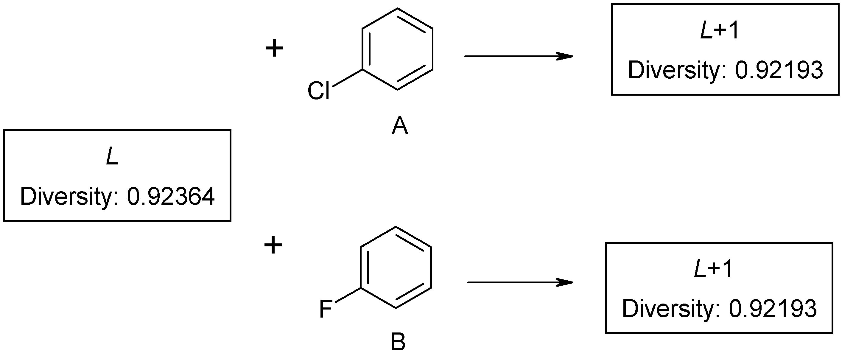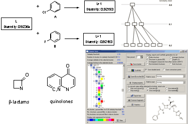It also results in inaccuracies in the process of diversity sorting, which is demonstrated by Figure 2. The first compound L is selected as a probe molecule. There exists another pair of compounds (A and B) with identical diversity to probe molecule. They contain the same number of fragments – both new and the existing ones. Thus, any of the two compounds with the same diversity can be selected as the second probe by diversity sorting. The remaining molecule is placed in the end of diversity sorted set and cannot be selected as a probe molecule. Such ambiguity may be extended by the third, fourth compound, and so on. If dataset L contains few aromatic fragments and no halogens, it makes no difference, which compound A or B, is selected (Figure2). This problem was described as ties in proximity [19].

Figure 2. Ambiguities in Maximum Dissimilarity Selection algorithm.

Figure 2. Ambiguities in Maximum Dissimilarity Selection algorithm.

However, this is is important for subsequent calculations. If structure A is selected as a probe molecule, the cluster will mainly be formed by chloroaromatic compounds, while fluoroaromatic compounds may be assigned to a different cluster. Thus, there exist several methods of screening datasets to select L structures. However, if datasets with identical order of compounds are used, the algorithm returns the same structures L. This results in deterministic clustering. To make initial datasets identical, 12-byte hash codes [20] are generated for chemical structures. The fixed-length chemical structure encoding has advantage compared with variable-length (InChI[21], SMILES[22]), because of calculations with fixed-length variables are simplest and consuming less time. Then hash values are sorted in a decreasing order. Such sorting of datasets leads to deterministic results in most cases. The mistakes, which arise due to rounding error and measures on discrete data, are compensated for identically ordered datasets. There is small, but nonzero probability, that different structures have identical 12-byte hash code, which is used for sorting. Such event was never observed by us for databases, which contain some millions of available compounds.

The suggested algorithm involves the following steps:

1. Generating hash codes for all chemical structures in the initial dataset. At this stage all topological duplicates are removed automatically - they have identical hash codes.

2. Setting the initial number of clusters (K=1) and starting the similarity threshold (R=0.0).

3. Requesting the number of steps (Nst) for further calculation of the difference between similarity thresholds (Rd=1/Nst). The Nst value equals the number of levels in the resultant hierarchy.

4. Diversity sorting in each cluster C for similarity threshold R. Forming the set of probe molecules [14] S, namely:

a. Selecting the compound most dissimilar to all molecules in the cluster and putting it into set S.

b. Selecting compound M which is the most dissimilar to structures in set S (MinMax diverse selection). At first step, the compound M is most dissimilar to single compound, selected in step a). At next steps M has maximal average distance to all compounds in set S.

c. Calculating similarity of compound M to all compounds in set S. If maximal similarity ratio is greater than R+Rd, set S remains unchanged. Otherwise, compound M is added to set S. The algorithm then proceeds to Point b for selecting the next compound.

The number of compounds in probe set S is equal to the number of clusters plus the number of singletons. Thus, the number of resultant clusters is not determined beforehand-it is calculated from diversity of dataset.

5. Calculating similarity of each remaining compound to compounds in set S. Assigning compounds to the cluster with maximal similarity.

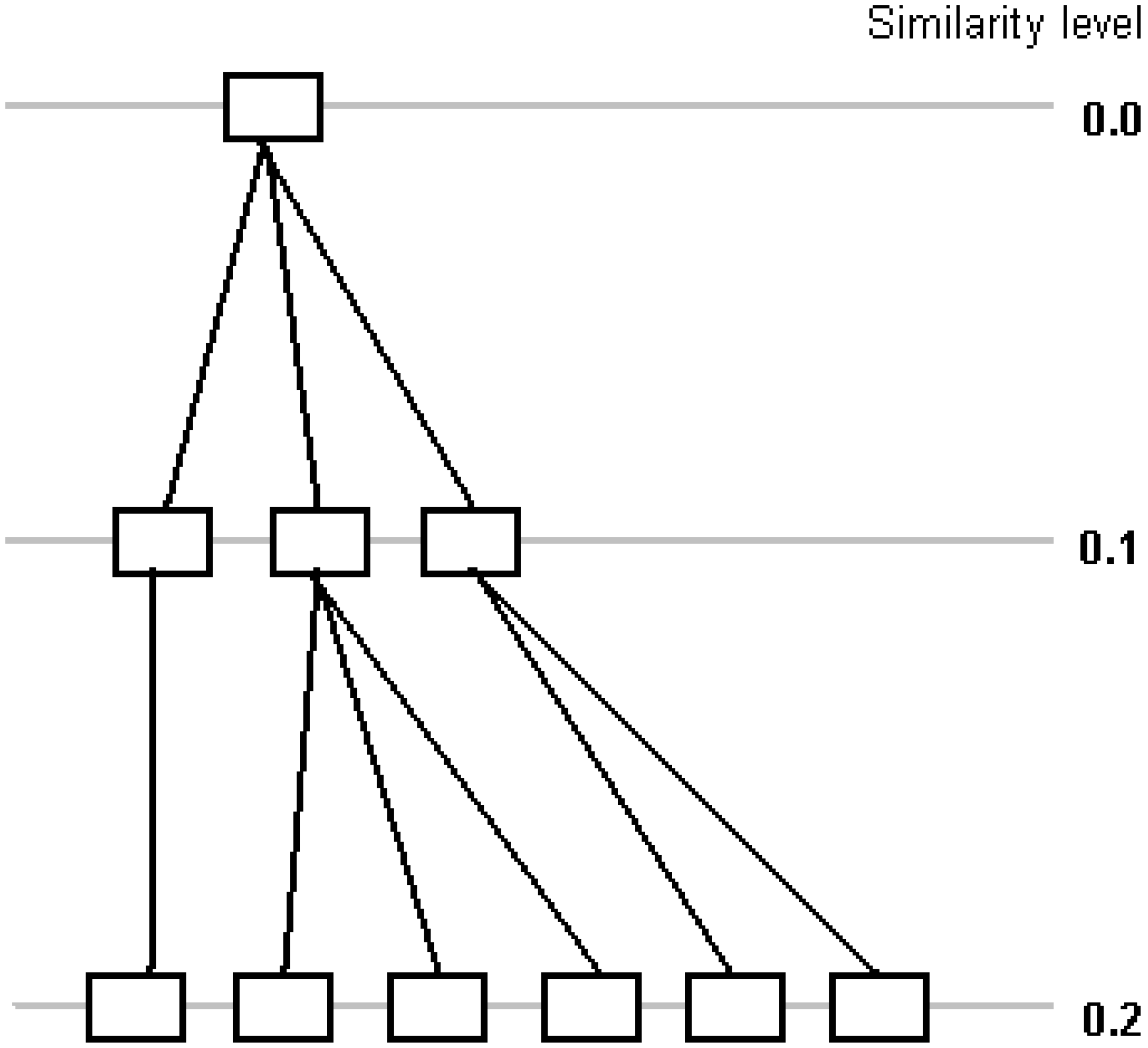
6. Setting similarity threshold (R=R+Rd). Assigning this value to all clusters generated from cluster C. The algorithm then proceeds to Step 4. It is repeated until similarity threshold reaches value 1 (Figure 3).

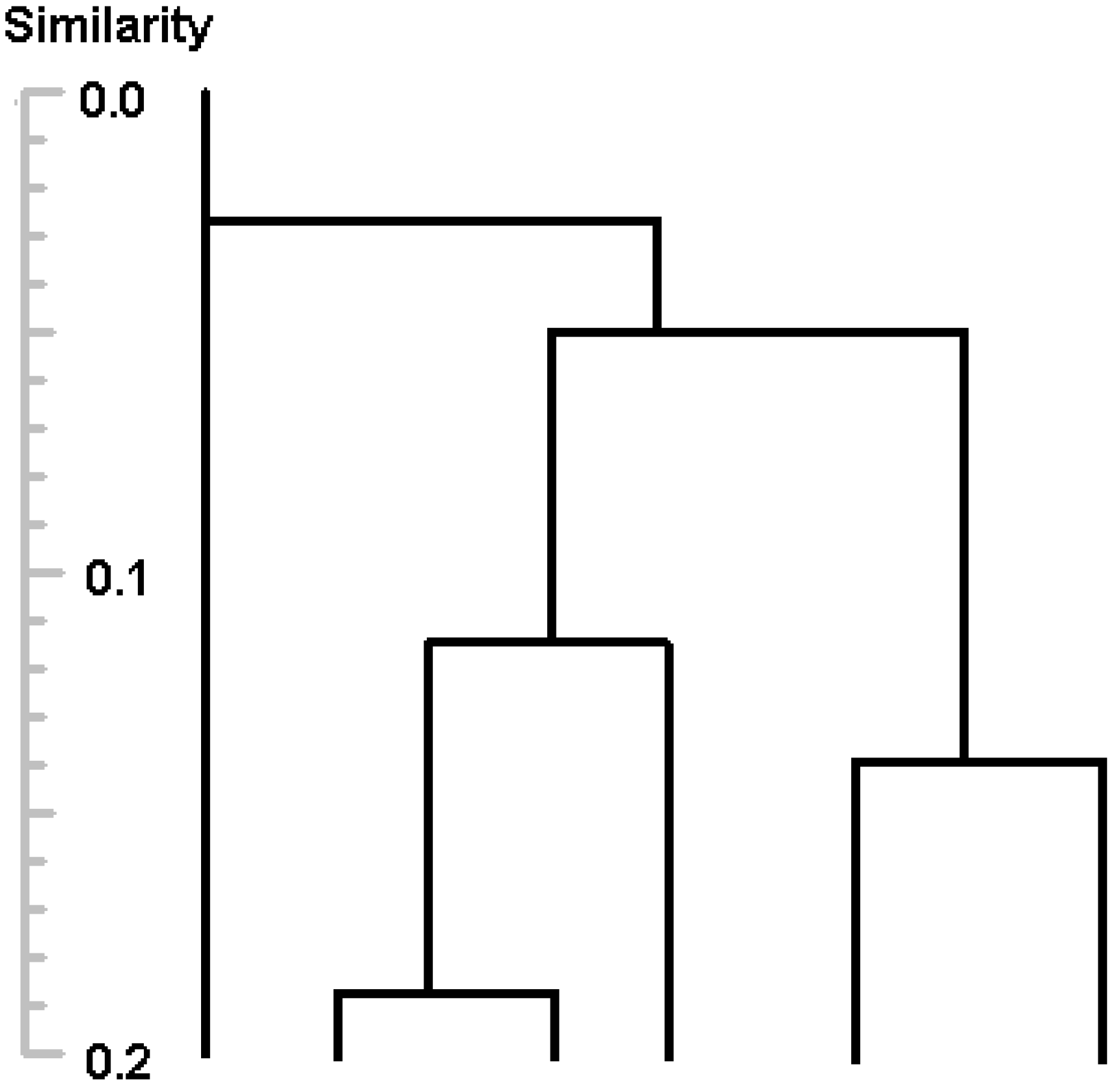
Figure 3 shows a part of the tree generated by proposed algorithm (compare with Figure 1). Many clusters are generated at each step, while traditional divisive hierarchical clustering algorithms divide a cluster into two at each step [23] or combine two clusters into one in agglomerative algorithms. Information about exact value of similarity of a pair of clusters is lost, but performance is increasing, since one step is used instead of several steps to divide a cluster.

Figure 3. Divisive clustering with Rd=0.1 (10-step clustering).

Figure 3. Divisive clustering with Rd=0.1 (10-step clustering).

2.1.2 Details of the algorithm creation

2D molecular structural fragments are used for calculating a bit vector required for molecular similarity calculations. The described algorithm uses circular, not linear, fragments with a variable sphere radius around the selected atom [24,25,26]. The sphere radius is a topological distance between the central atom and the maximally remote one. Value 1 is assigned to the length of each bond. Central atoms are selected one after another to split a molecule into spherical fragments. Then fragments with sphere radius 1, 2, etc. are sorted in succession. The suggested algorithm makes it possible to use information on the cycle size. To do this, an additional cycle size attribute was assigned to a chemical bond in addition to the bond order. This is a distinguishing feature of the algorithm. The single bond in the aliphatic chain differs from the single bond in cyclopropane, which, in turn, differs from that in cyclopentane. If a bond belongs to two rings, a smaller size descriptor is used. Such distinctions are not made for cycles of size 6 and higher. This splitting method is also rational from the point of chemistry – it accounts for reactivity of small cycles. The suggested algorithm distinguishes bonds in 5 and 6-membered aromatic rings [20]. Each compound is checked for the presence of a fragment to form a bit vector. If the fragment is present, 1 is assigned to the corresponding component of the bit vector, otherwise the value is 0.

In earlier studies [27], we found that a sphere with radius 2 is sufficient for molecular similarity and diversity calculations. On average, each compound in the studied databases has 35 unique fragments [20]. A fragment is hashed into the 12-byte variable [20] to form key values. These values are sorted and stored in memory to form dictionary of all fragments. One cannot get any connection matrix from hashed value, but, optionally, connection matrix can be stored at hard drive with corresponding hashed value. It was experimentally found, that large, diverse databases contain several hundreds of thousands of unique fragments. So, the dictionary never exceeds 12M RAM and this value does not affect the calculation performance. The use of the dictionary of a large size (some hundred thousands of fragments) instead of fixed-length fingerprint is the main difference from circular SciTegic fingerprints [28] which has fixed restricted length.

The dictionary is formed during run-time when reading the database. Indexes of fragments in the dictionary are calculated and stored for each compound. To define similarity between two compounds, the numbers of identical and number of different indexes in the glossary are calculated. It allows considerable increasing of computer memory usage efficiency. Thus, 140 bytes of RAM are required on average to store screens for a single compound. Using this type of storing information allows PC RAM to upload the dataset of some millions of compounds.

To find indexes of fragments for new compound quickly, the dictionary is sorted and bisection search algorithm is used. If a fragment is not found, it is added to dictionary. In this case re-sorting is required to use bisection search algorithm, which decreases performance. To improve the performance it was suggested [29] to re-sort dictionary after several fragments addition. Non-sorted fragments in dictionary are compared with probe value step-by-step. Optimal productivity is achieved by sorting after addition of 128 fragments approximately [29]

The cosine measure was used to calculate similarities between compounds I and J:

$$SIMILARITY(I,J)=\frac{{\displaystyle \sum _{K=1}^F{M}_I(K)\times M_J(K)}}{\sqrt{{\displaystyle \sum _{K=1}^F{M}_I{(K)}^2\times {\displaystyle \sum _{K=1}^F{M}_J{(K)}^2}}}}$$

where M_I and M_J are bit vectors for compounds I and J, F is the number of components in the bit vector. Cosine coefficient allows the diversity sorting with fast centroid algorithm [30], but it is more rarely used than the commonly applied Tanimoto [31] metric.

Cosine similarity coefficient can vary from 0 (totally dissimilar compounds) to 1 (identical compounds). This variability range is divided into several steps, the number of steps being user-defined parameter. For example, if the number of steps equals 10, then the similarity thresholds are 0.0, 0.1, 0.2…0.8, 0.9, 1.0. Several clusters are generated for each level. The similarity of each compound to a probe molecule in the cluster equals or exceeds the predefined similarity threshold.

With the increasing similarity value, the cluster splits into several clusters forming a cluster tree. Diversity sorting is repeatedly performed in each cluster to select a set of probe molecules. One-time sorting of the input database may not be sufficient because of the order of compounds in the sorted set is changed after removal of selected compounds. Diversity sorting is a reiterated procedure.

As a result of splitting clusters in building hierarchical tree, some compounds’ similarity to the probe molecules may be below the predefined similarity threshold. Such compounds are joined with the set of probe molecules to form a new cluster; therefore the probe set can be expanded dynamically. Expanding of the probe molecules set is regarded as an additional source of non-deterministic clustering.

Probe molecules that have no neighbors form singletons. Each singleton may form a new cluster if similar structures are added to the database under study. Singletons may be treated individually or as assigned to nearest clusters.

2.1.3 Memory usage and scaling

The results of clustering for every similarity threshold are stored in memory as an integer number for each chemical structure. Structures with identical numbers belong to the same cluster. Estimated memory requirements to run clustering are:

1. Dictionary of fragments: 12*F bytes, where F is the number of different structural fragments in the database. The number of fragments depends upon diversity of database. For 2M database the typical value of F is about of 700,000

2. The centroid vectors of weights and sorted dictionary: 16*F bytes.

3. Molecular screens as indexes in glossary: 4*N*AvgFrag+4*N bytes. Here N – the number of chemical structures, AvgFrag-average number of fragments per compound, which is equal to 35 for databases under study. Screens are stored in linear array; the number of screens for each chemical structure is also stored.

4. Results of clustering: 4*N*Nst bytes.

These memory requirements should be treated as minimal because of a lot of memory is used for auxiliary information (addresses of binary records with chemical structures, tree view graphical control etc.). One should note linear growth of resources used with the database size.

To estimate the overall processing, we assume that each cluster is divided into k cluster uniformly at each similarity threshold. Single cluster exists at similarity threshold 0, while for last threshold (Nst threshold level, similarity=1) there exist N clusters. So, k=exp(ln(N)/Nst) and the number of clusters at each i-th level (i=0..Nst) is m_i=kⁱ=exp(ln(N)*i/Nst). The size of the i-th threshold is d_i=N/kⁱ=exp(ln(N)*(Nst-i)/Nst). Both k and d_i depend not exponentially, but almost linearly on the dataset size N.

The centroid vector is calculated for each cluster, which requires d_i*AvgFrag additions. The distance of each compound from centroid (scalar product) is calculated, it includes d_i*AvgFrag multiplications and d_i*AvgFrag additions. The advantage of non-zero components store should be pointed out. The centroid vector (F) has large dimensions (hundreds of thousands of components), though, taking into considerations non-zero elements (AvgFrag) only, it amounts to some tens components. The calculation time is proportional to the i-th cluster size d_i and the average number of nonzero screens equals to d_i*AvgFrag.

Subsequent operations are: quick sorting of distances (calculation time is proportional to d_i*ln(d_i)), putting the first compound in probe set S, and then selection of most diverse k-1 compounds. It should be noted, that modifications [29] were implemented for compounds selection, namely:

Indexes in glossary (their number equals AvgFrag) are used for fast scalar product calculation

For selection of the most diverse compounds from cluster to already selected ones in probe set S it is enough to calculate similarity of few first compounds at the beginning of sorted array only.

The number of structures, for which similarities are calculated, is proportional to ln(d_i), therefore the total time for selecting first diverse k compounds is proportional to k*ln(d_i)*AvgFrag.

To assign remaining compounds to k clusters, scalar products for each remaining (d_i-k) compounds are calculated with k probes. The calculation time is proportional to (d_i-k)*k*ln(d_i)*AvgFrag. This procedure is the most time-consuming. Assuming d_i>>k (large datasets), the time for single-cluster processing is proportional to AvgFrag*k*d_i*ln(d_i)_. The time for building up all clusters for i-th similarity threshold is:

time(i) =O(ln(N)*(Nst-i)*AvgFrag*exp^{(ln(N)*(Nst+1)/Nst)}/Nst).

Taking Nst>>1, one can evaluate overall processing time to construct clusters tree as:

${\displaystyle \sum _{i=0}^{i<Nst}time(i)}=O(N\ast ln(N)*AvgFrag*Nst/2)$.

Square dependence of calculation time on dataset size in divisive hierarchical clustering algorithms is given in [6]. Modern algorithms have time dependency better than O(N*ln(N))[32]. There are three improvements, which help to perform calculations faster in proposed algorithm:

Division of a cluster into many clusters but not into two as in traditional divisive cluster algorithms.

Storing and using non-zero components only for centroid and scalar products calculations

Fast selection of most diverse compounds to make probe dataset.

Memory requirements and overall processing should be compared with other algorithms applied to large databases (> 1M size) described in the literature [7,13]. Some databases were successfully clustered with a Xeon Intel 3 MHz processor with 2G RAM [13] running Linux, but the memory used and algorithm complexity were not reported. From the time required for clustering different size datasets, one may conclude the algorithm complexity to be O(N), and minimal memory requirement to be 124*N bytes (from 988-bit fingerprint length). This value is some smaller than that used in our work 140*N bytes (see above), required to store non-zero indexes in glossary. The complexity of algorithm [13] is better than that proposed in this work, but the calculation time normalized by processor frequency has the same order or, is even larger for small datasets. It should be pointed out that estimated complexity and calculation time in [13] are reported for single similarity threshold-algorithm [13] without cluster tree building.

Minimal memory, estimated for [7] is 256*N bytes (2048-bit Daylight fingerprint). This value is greater than that used in our work (140*N). Estimated algorithm complexity is O(N*ln(N))[7], which is better than ours, but the calculation time was much larger - 16 days on a SGI Origin 300 single-processor computer for a 1.1M dataset. High speed of scalar product calculation and generation of multiply clusters at each step might explain why the algorithm with the worst complexity has a lower calculation time. In reality, 2048 multiplication and additions are required to calculate scalar product for a Daylight fingerprint [7]. In the proposed algorithm only AvgFrag(some tens) additions and multiplications are required.

2.1.4 Program performance

The Aurora Fine Chemical database [33] (AURORA) was used to evaluate clustering program performance. The database included 4,000,000 records of low-molecular compounds, including structures, which contain fragments of antibiotics (beta-lactams or quinolones). Datasets of different size were prepared by random selection of compounds from 4M Aurora database. The tests were performed using an ASUS laptop computer equipped with an Intel Core Duo, 1.83GHz processor and 2Gb RAM. The main purpose of this section was to estimate the employment of real resources, time of calculation for datasets of different size and to check, whether the proposed algorithm is deterministic. For that input datasets were varied by size and sorting methods. If an algorithm is deterministic, identical trees have to be generated from datasets, sorted by different fields. Sorting by supplied IDNUMBER can be treated as random. Calculation times required to complete clustering and the number of clusters for databases of different size and different sorting are displayed in Table 1.

Table 1. The result of clustering for databases of different size (Nst=10, Minimal Cluster Size=2) and sorted by different way.

Database size Ordered by	Calc. time	No. clusters for similarity threshold
		0.1	0.2	0.3	0.4	0.5	0.6	0.7	0.8	0.9
1,000,000 IDNUMBER	4h 00m	103	2155	17943	65203	125147	167505	184483	178385	137138
1,000,000 Molweight	4h 13m	101	2155	17943	65203	125147	167505	184483	178385	137138
2,000,000 IDNUMBER	14h 08m	120	2779	25345	105025	224140	314893	361163	376966	317183
2,000,000 Molweight	13h 41m	120	2779	25345	105025	224140	314893	361163	376966	317183
2,500,000 IDNUMBER	Cannot cluster – out of resources

Table 1. The result of clustering for databases of different size (Nst=10, Minimal Cluster Size=2) and sorted by different way.

Database size Ordered by	Calc. time	No. clusters for similarity threshold
		0.1	0.2	0.3	0.4	0.5	0.6	0.7	0.8	0.9
1,000,000 IDNUMBER	4h 00m	103	2155	17943	65203	125147	167505	184483	178385	137138
1,000,000 Molweight	4h 13m	101	2155	17943	65203	125147	167505	184483	178385	137138
2,000,000 IDNUMBER	14h 08m	120	2779	25345	105025	224140	314893	361163	376966	317183
2,000,000 Molweight	13h 41m	120	2779	25345	105025	224140	314893	361163	376966	317183
2,500,000 IDNUMBER	Cannot cluster – out of resources

The AURORA database contains unique structures. However, stereoisomers can occur in small amounts. Therefore, we used 999,756 and 1,999,335 records with topologically unique structures for the tests. The calculation time did not bypass acceptable limits even for the largest databases. It is important to note that hash codes sorting have generated the identical number of clusters for databases, formerly sorted by various methods. This proved that clustering algorithm was deterministic.

Test calculations were performed for a 1,000,000 database, ordered by IDNUMBER, but with different number of steps: Nst=5 and Nst=20. The calculation times were 1 hours 52 minutes and 9 hours 38 minutes, respectively. As it is expected (see Memory Usage and Scaling section), the calculation time grows approximately linearly with increasing Nst.

The described algorithm was created as a program for Windows 32 platform. The program is a part of CheD chemical database management system [34]. Clustering is finalized by displaying the tree view. Each tree node displays the number of compounds in the cluster. The number of clusters may be huge, for example, after clustering of database with 2,000,000 records 1,727,615 clusters were generated (Table 1). Therefore, the tree view is populated dynamically to minimize processing time and resources. Program has tools for singleton handling (export to file or addition to nearest cluster) and for fuzzy cluster analysis [35] (list of overlapped compounds can be obtained).

Results of the antibiotics classifications cannot be compared with standard algorithms for the same size of dataset, because of they were designed for small chemical databases.

2.1.5 Validity of clusters and antibiotics classification

Applicability of clustering results for chemical compounds classification is the best confirmation of clusters’ validity and the correct choice of a clustering algorithm [6,8]. Antibiotics were classified to evaluate the efficiency of clustering.

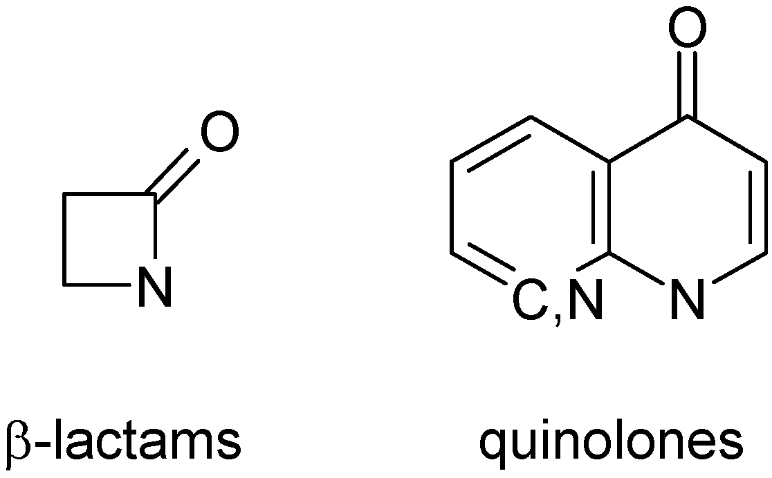
Figure 4. Main classes of antibiotics under study.

Figure 4. Main classes of antibiotics under study.

A database of 3,249 compounds with anti-bacterial activity (ABIO) [36] was used for model calculations. After removing duplicate structures and stereoisomers, the ABIO database was reduced to 1,183 topologically unique structures. It contained 868 β-lactams, 325 quinolones (Figure 4), several compounds with both elements, and 37 other antibiotics (macrolides, etc.). The content of the ABIO database was clustered to produce six clusters at 0.1 similarity threshold and 78 clusters at 0.5 threshold. Clusters at 0.1 threshold are mixed: each contains both quinolones and β-lactams. One should expect such results: antibiotics contain several substitutents which are bigger than a β-lactam ring and affect more bits in the screen vector. On the other hand, the non-informative rings (pyridine) produce structural screens, which are part of quinolones.

To estimate possibilities of classification of antibiotics in large databases, the ABIO database was combined at random with 999,994 unique structures from the AURORA database. Thus, the input database (TESTDB) with 1,001,177 records was formed. The field Activity was created for TESTDB. Its value was set to 1 for all records from ABIO and to 0 otherwise.

The number of steps was defined as 10 (Nst = 10) to create similarity thresholds of 0.1, 0.2, etc. The minimal cluster size was set to 2. The obtained cluster tree displayed information of 879,609 clusters and 8,672,957 chemical structures at different similarity thresholds! TESTDB database contained only 0.12 of target compounds. The large size of the database and the low probability of discovering target compounds made manual analysis of the cluster tree absolutely inapplicable. Data preprocessing, filtering, and visualization tools were required for better assessment.

Filtering could be performed by assigning a variable value for some parameters. For TESTDB database the field Activity value was used for visualization. Conditional colors were applied to display the values as described in [37]. The average value of the selected parameter was calculated for each cluster and displayed as an icon of appropriate color at tree view control.

Two types of cluster filtering: minimal and representative, were created for cluster tree reduction. Both filters used external properties (Activity value for the described calculations). The range of target properties was defined by the user. Two types of filtering differ by applicability of a predefined range of target properties.

Minimal. The cluster is displayed if one chemical structure has a property value in the specified range.

Representative. The cluster is displayed if more, than 50% of structures has property values in the specified range. Such criterion divides clusters into two groups: active and inactive. We do not use more complex statistical criteria [38], which divide clusters into several groups and are used for experiment optimization only.

Both types of filtering visualized selected clusters as well as parent clusters, even if parent clusters did not satisfy filter conditions. The data obtained as a result of TESTDB clustering were summarized in Table 2. It also displays the results of filtration using Activity field in the range 0.9-1.0. Calculation time was 3 hr 59 min. The structures not assigned to clusters in the Unfiltered field form singletons.

Table 2. Results of clustering TESTDB with Nst=10 and minimal cluster size=2.

Similarity threshold	No. of clusters (upper value) and number of compounds in clusters (lower value)
	0.1	0.2	0.3	0.4	0.5	0.6	0.7	0.8	0.9
Unfiltered	103 1001174	2186 1001030	18024 998525	65560 980144	125426 924788	167529 833572	184916 715498	178515 567843	137349 649206
Minimal	41 938335	133 321443	169 25978	173 3636	179 1389	203 1171	233 1047	265 899	204 544
Representative	34 918634	88 136643	118 8359	143 1565	163 1238	192 1127	228 1030	263 893	203 541

Table 2. Results of clustering TESTDB with Nst=10 and minimal cluster size=2.

Similarity threshold	No. of clusters (upper value) and number of compounds in clusters (lower value)
	0.1	0.2	0.3	0.4	0.5	0.6	0.7	0.8	0.9
Unfiltered	103 1001174	2186 1001030	18024 998525	65560 980144	125426 924788	167529 833572	184916 715498	178515 567843	137349 649206
Minimal	41 938335	133 321443	169 25978	173 3636	179 1389	203 1171	233 1047	265 899	204 544
Representative	34 918634	88 136643	118 8359	143 1565	163 1238	192 1127	228 1030	263 893	203 541

Figure 5 shows the clusters tree after Representative filtering. The chart is more compact compared to non-filtered clustering. Due to smaller number of tree nodes, run-time operations (expanding, collapsing) required less time, than for unfiltered data.

Analyzing the cluster tree, one can conclude that the antibiotics have formed clusters, starting from similarity threshold equal to 0.2 and these clusters still exist at 0.9 similarity threshold. Clusters multiply with increasing the similarity threshold (with exception of similarity threshold 0.9). Clusters reduce in size and become more distinct in similarity of structures.

Figure 5. Implementation of Representative filter for TESTDB clusters tree view.

Figure 5. Implementation of Representative filter for TESTDB clusters tree view.

To illustrate it, a tree, generating cluster, selected in Figure 5 (number of compounds=65) was investigated. A modified algorithm [39] was used to find a common independent substructure set for a cluster. An independent substructure set is a set of substructures of maximal size, which are common for selected dataset and none of them is a subgraph of another.

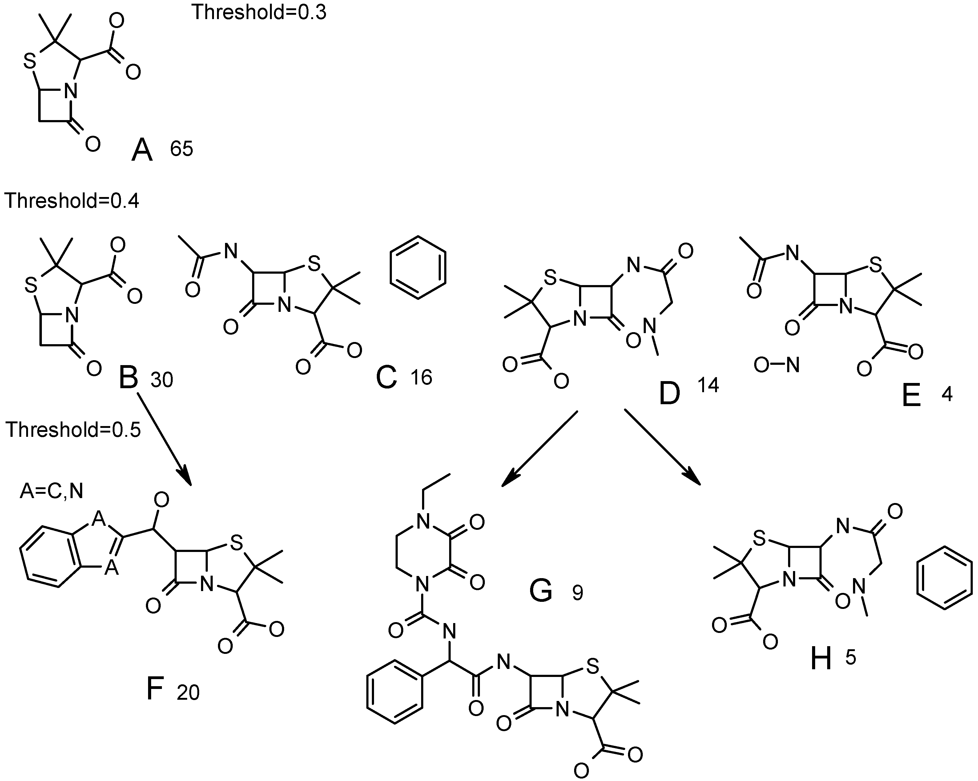
Figure 6. Common fragments, found for clusters at different similarity threshold. Number of compounds in each cluster is displayed. Parents for structures F, G, H are shown with arrows.

Figure 6. Common fragments, found for clusters at different similarity threshold. Number of compounds in each cluster is displayed. Parents for structures F, G, H are shown with arrows.

A cluster with 65 structures at similarity threshold=0.3 (Figure 5) has the maximal common fragment A (Figure 6). It forms four clusters B-E at similarity threshold 0.4. Together they contain 64 compounds, plus one compound forming a singleton at 0.4 threshold. A maximal common fragment is identical for clusters C and E. They are distinguished by presence of phenyl at different positions in C and by presence of nitrogen-oxygen bond in E. Cluster B is not specific and contains the same common fragment as cluster A.

At threshold 0.5 cluster E remains unchanged. Cluster D forms two clusters – G and H (Figure 6). One of them (G) is distinct and does not change up to 0.8-similarity threshold. Cluster C produces a cluster with 13 structures (three singletons), the common fragments being the same as in C, but hydroxyphenyl is detected as a common fragment instead of phenyl. Finally, cluster D produces two clusters; one of them (F, Figure 6) is distinct. This cluster leaves singleton at similarity threshold 0.6 and forms a cluster with 19 compounds, where atom A is equal to nitrogen (Figure 6). This cluster (A=N) remains unchanged up to threshold 0.8. The second cluster, formed from B at 0.5 threshold (the size was eight compounds), is not distinct and is divided into three small clusters and two singletons at 0.6 threshold.

Thus, both distinct and non-distinct clusters are formed at similarity thresholds 0.5. The more the similarity threshold, the more distinct clusters are. But at high values of similarity threshold a lot of small-size clusters and singletons are generated. The more singletons (or small-sized clusters) in the final data, the greater the probability of incorrect classification of compounds in external databases is. In reality, a singleton can form a new cluster if a number of similar compounds are present in the external database. But, if this singleton would be absent in ABIO database, then compounds similar to the above singleton might be classified in other clusters with common, but non-informative structural fragments (phenyl, furyl, etc). If such clusters are marked as inactive, a wrong conclusion may be reached. Thus, the more the number of singletons, the more prediction possibilities are sensitive to initial ABIO content. Additionally, some compound may not be assigned to any cluster at high similarities thresholds, therefore no conclusion about their activity can be made.

The number of singletons increases with increasing similarity threshold and the number of clusters are reduced at high similarity threshold (0.9). It is clear, that there is an optimal similarity threshold for classifying antibiotic from random structures. To select such a threshold, it is necessary to study two types of classification errors.

1) Error1. Compound from ABIO database was not present in a Representative antibiotic cluster. Such compound might be a singleton. Alternatively, it was present in the cluster formed by compounds from AURORA database mainly.

2) Error2. Compound from AURORA database with Activity=0 was included into the Representative cluster of antibiotics (Activity=1).

After filtering two lists of compounds corresponding to both kinds of classification errors were formed automatically for the selected similarity threshold. Error 2 requires special consideration. All compounds from AURORA database were assumed to have 0 Activity value. However, it was not true. AURORA database combined all classes of compounds, antibiotics among them. Therefore, occurrence of such structures in the antibiotics clusters is not accidental. Since the bioactivity data for AURORA database were not available, the structures with β-lactam or quinolone fragments of antibiotics (Figure 4) cannot be treated as Error2.

The number of representative clusters (Row 2 in Table 3) should not be compared with the results of representative filtering (Table 2). At low similarity thresholds Table 2 displays non-representative clusters. They are parent clusters for representative ones at high values of similarity threshold. Non- representative clusters are included to maintain the cluster tree integrity.

Cluster overlapping data are displayed in rows 8 and 9 in Table 3. A quarter of AURORA structures are overlapped by ABIO clusters and all ABIO structures are overlapped by AURORA clusters at similarity threshold 0.2. Almost non-overlapped clusters occur when the similarity threshold is 0.7 and higher. One may conclude that the reason of such huge overlapping results from the nature of antibiotics. The β-lactam fragment is too small and gives a small number of non-zero components in bit vector, as well as another substituents of approximately equal size. A lot of non-informative substituents (pyridine, furyl, etc) satisfy these conditions. So, if a β-lactam antibiotic would have two or more substituents (this is true in the majority of cases), it might be assigned to a cluster which contains other chemical structures with the same substituents. Contrary to this, if a structure without a β-lactam ring has two or more substituents, identical with some antibiotics, it may have high similarity being in single or overlapped clusters. The quinolone fragment is larger, but it gives a lot of non-zero bit vector components, which are identical with non-informative phenyl and pyridyl substituents. This also results in overlapped clusters. To reduce overlapping, one can restrict fragments and leave informative ones only. But such approach reduces application of the clustering algorithm: non-informative fragments may have great significance in other tasks.

Table 3. Classification errors at different similarity thresholds. The smaller are the values in Rows 3 and 6, the better classification is. The term “Representative clusters” stands for the number of clusters containing over 50% compounds from ABIO database.

1	Similarity threshold	0.2	0.3	0.4	0.5	0.6	0.7	0.8	0.9
2	No. representative clusters	8	70	117	151	185	225	263	203
3	No. non-clustered ABIO structures (Error1)	734	222	144	147	169	199	304	645
4	No. clustered AURORA structures (Error2)	238	154	109	73	32	25	14	3
5	AURORA structures, having β-lactam or quinolinone fragments	27	94	85	66	27	22	13	3
6	4 and 5 difference (“pure” Error2)	211	60	24	7	5	3	1	0
7	% successfully classified ABIO compounds	38.0	81.2	87.8	87.6	85.7	81.0	79.1	45.5
8	No. of AURORA structures (top) and No. of AURORA structures without antibiotic fragment (bottom), overlapped with representative clusters	242967 238570	152192 149733	47571 45815	7483 7429	609 321	153 1	45 0	8 0
9	No. of ABIO structures, overlapped with non-representative clusters	1183	1158	1062	798	344	76	10	5

Table 3. Classification errors at different similarity thresholds. The smaller are the values in Rows 3 and 6, the better classification is. The term “Representative clusters” stands for the number of clusters containing over 50% compounds from ABIO database.

1	Similarity threshold	0.2	0.3	0.4	0.5	0.6	0.7	0.8	0.9
2	No. representative clusters	8	70	117	151	185	225	263	203
3	No. non-clustered ABIO structures (Error1)	734	222	144	147	169	199	304	645
4	No. clustered AURORA structures (Error2)	238	154	109	73	32	25	14	3
5	AURORA structures, having β-lactam or quinolinone fragments	27	94	85	66	27	22	13	3
6	4 and 5 difference (“pure” Error2)	211	60	24	7	5	3	1	0
7	% successfully classified ABIO compounds	38.0	81.2	87.8	87.6	85.7	81.0	79.1	45.5
8	No. of AURORA structures (top) and No. of AURORA structures without antibiotic fragment (bottom), overlapped with representative clusters	242967 238570	152192 149733	47571 45815	7483 7429	609 321	153 1	45 0	8 0
9	No. of ABIO structures, overlapped with non-representative clusters	1183	1158	1062	798	344	76	10	5

There are different ways to select optimal similarity threshold, like penalty functions [40] or stopping rules [41]. In these approaches a substantial change in properties take place at optimal threshold. One may observe that the majority of antibiotics were assigned to representative clusters at similarity threshold 0.4. Only 144 antibiotics (12.2%) remain unassigned, but 24 compounds from AURORA database without antibiotic fragments (Table 3) were erroneously classified as active (Error2). Approximately 87% antibiotics were successfully classified at similarity thresholds 0.5 and 0.6. The number of compounds in Error2 group at similarity threshold 0.5 (seven compounds) and 0.6 (five compounds) was considerably less than at similarity threshold 0.4. This should be treated as stopping criteria [41]. Also, if one considers Error 1 as penalty function [40], clustering should be stopped at similarity threshold 0.4. On the other hand, the fuzzy clustering approach gives better values for 0.6 similarity threshold. 87.6% of the antibiotics were classified at 0.5 threshold, while a slightly lesser value (85.7%) was observed for 0.6. The 0.5 similarity threshold produces a lesser number of singletons and small-sized clusters, which, in turn, diminishes the prediction possibilities. On the other hand, a fuzzy clustering approach (rows 8 and 9, Table 3) gives a better value for 0.6 threshold (0.03% overlapping), than for 0.5(0.74%). At 0.7 threshold clusters become almost distinct, but the small average cluster size (3) makes the data unsuitable for external database classification. Thus, a similarity threshold of 0.6 can be considered optimal for classification of antibiotics. There is some ambiguity in selecting best the threshold among the two values 0.5 and 0.6. The data for 0.5 and 0.6 thresholds are very similar, and it is impossible to determine an optimal threshold with precision better than 0.1 in the problem under consideration, so, it is no good to increase number of steps (Nst) for antibiotic classifications because of different criteria give different optimal similarity thresholds, the difference being greater 0.1.

The program allows saving probe molecules for the selected similarity threshold in SD files for further clustering of external databases. SD files with probe molecules and singletons for similarity threshold 0.6 are available in this work. Singletons may form clusters in databases with other content. Saved data can be used for classification of antibiotics in large databases with random content, like PubChem [42].

The validity of the obtained set of clusters was confirmed. 85.7% of the studied compounds were successfully classified with 0.4% of error. Such result is remarkable as classification was performed at a very high noise level: TESTDB database contained 0.12% antibiotics only.