1. Introduction
Computational molecular biology, or, shortly, computational biology, is a research field which studies the solution of computational problems arising in molecular biology. It is a discipline whose questions can often be posed in terms of graph theory, network flows, combinatorics, integer and linear programming problems. Furthermore, some problems have been attacked by statistical approaches, probabilistic methods, hidden Markov models, neural networks, and many other solving techniques.
The field of computational biology is today about twenty years old. In the very early years, computational biology was a topic of limited interest, because it was of limited practical impact. Many of the first computational biology papers were written by theoretical computer scientists and appeared in CS theory conferences. They contained long and complex proofs of NP-hardness for some “toy” version of real biology problems (e.g., protein folding in the 3D lattice for the HP protein model [
1]), or approximation algorithms with large approximation-ratios and/or exponential worst-case complexity.
There were two main limitations for these works to possibly be of real significance for the biologists and help them in solving their problems: (i) The models studied were simple abstractions of the real problems. These abstractions, much cleaner than the underlying problems, have nice mathematical properties that make them simpler to tackle. However, they are too detached from the real problems, so that their solutions are sometimes infeasible or suboptimal. (ii) The works were highly theoretical and understandable by computer scientists only. Many papers lacked experimental parts, or all experiments were done on simulated data, quite different from the real data that the biologists had to deal with.
The exponential growth in the availability of genomic data has increased the importance of computational biology over time. In turn, many researchers with different backgrounds have approached the field, and, today, computational biology papers are written not only by computer scientists and biologists, but also by statisticians, physicists and mathematicians, pure and applied. In particular, the apparently endless capability of computational biology to provide exciting combinatorial problems, has become very appealing to the Mathematical Programming/Operations Research community. In fact, many computational biology problems can be cast as optimization problems, to be attacked by standard optimization techniques.
The typical approach to tackle a computational biology problem is the following. First, a modeling analysis is performed, in order to map the biological process under investigation into one or more combinatorial objects (such as graphs, sets, arrays...). After the modeling phase, the original question concerning the biological data becomes a mathematical question about the objects of the chosen representation. Each object representing a tentative solution has a numerical weight associated with it, intended to measure its quality. The weight is proportional, loosely speaking, to the probability that the solution is the “true" answer to the original biological problem. The higher the weight, the more reliable a solution is. Where the weight is represented by some function , in order to find the best answer to the original biological problem, one has to solve the following optimization problem: find a solution which maximizes over all possible solutions.
Optimization problems have been studied for decades by the mathematical community, particularly within the field of Operations Research. Many successful techniques, going under the collective name of “mathematical programming”, have been developed over the past years for the effective solution of difficult (NP-hard) optimization problems. In this survey we list some of the many papers which have appeared over years that have tackled a computational biology problem by using a “mathematical programming approach” (in the broad sense explained below). In particular, we consider those papers which
- (1)
study a computational biology problem (even if as a secondary subject, or as one of the possible applications for a technique)
- (2)
employ, directly or indirectly, mathematical programming/OR techniques. For an example of indirect application, they may reduce the computational biology problem to a standard optimization problem, (e.g., Set Covering), solved, in turn, by mathematical programming techniques.
Perhaps the first such paper is by Alizadeh, Karp, Weisser and Zweig [
2], and showed how a particular
physical mapping problem (i.e., the problem of determining the order of some DNA markers on a given chromosome) can be cast as a special TSP problem, to be solved by standard TSP techniques.
Figure 1.
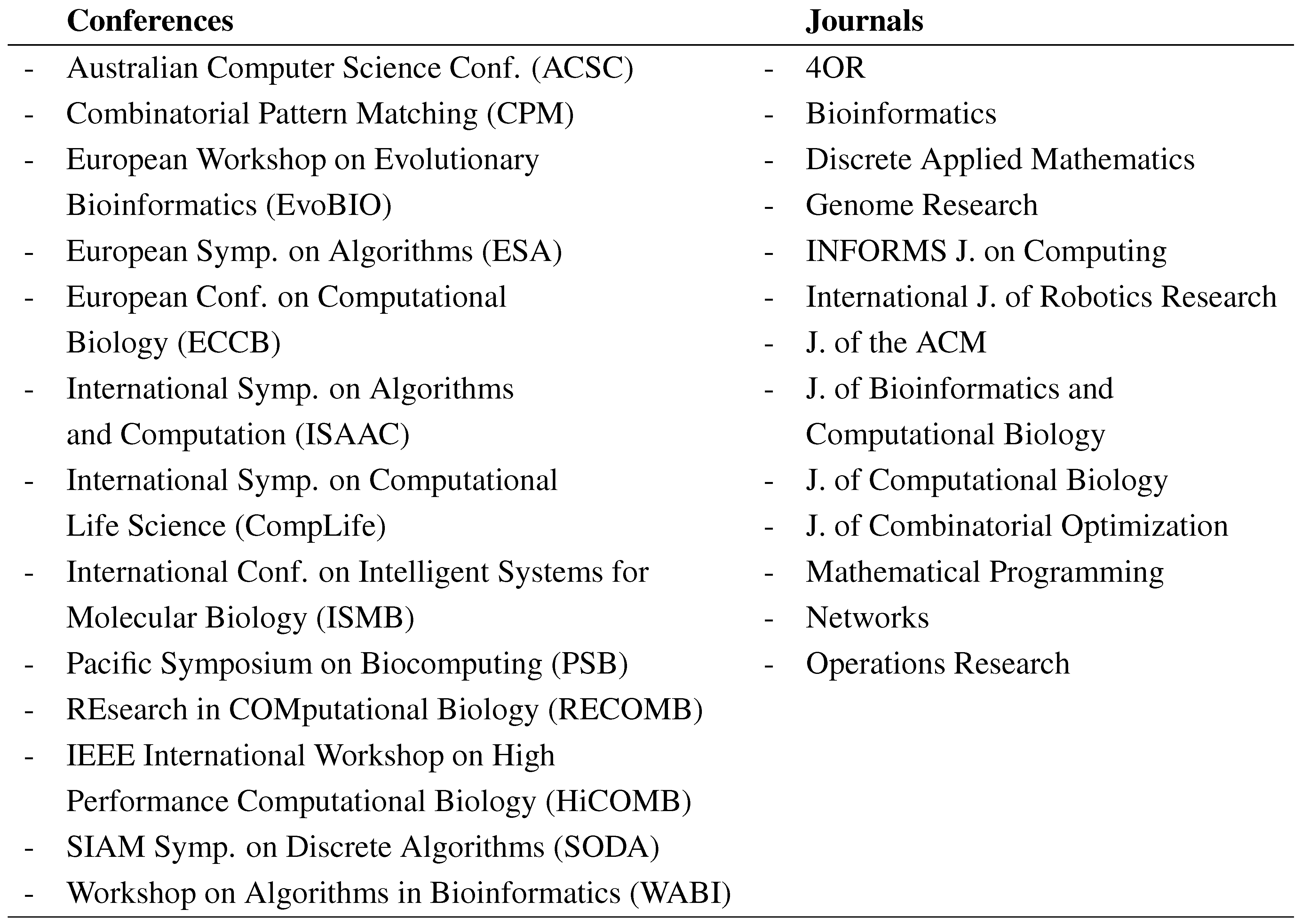
Conferences and journals publishing MP papers in CB.
Figure 1.
Conferences and journals publishing MP papers in CB.
In the years within 1995 and 2005 there were about fifty such papers published (many more, if we double count those papers that appeared first in conference proceedings and then in journals). The number of mathematical programming papers for computational biology went from one paper in 1995 to 25 in 2005. In
Table 1 we report the names of the journals and conferences on which these papers appeared.
The paper is organized as follows. In
section 2., we describe the underlying biological problems that are considered by the papers we survey. In order to establish a basic vocabulary, we give some introductory molecular biology notions and describe, in a necessarily simplistic way, a set of biology concepts and experiments. For a comprehensive description of molecular biology at an introductory level, the reader is refereed to Watson, Gilman, Witkowski and Zoller ([
3]), and to the web sites of the European Molecular Biology Laboratories, EMBL (
www.embl.org) and of the National Institute of Health, NIH (
www.nih.gov). The section introduces five main problem areas that are later used to group the papers by topic. These areas are:
sequence analysis,
hybridization and microarrays,
protein structures,
haplotyping,
evolution.
In
section 3. we consider the papers, grouped by the class of problems they study. We also classify the papers according to the type of approach employed. A list of the approaches considered is given at the beginning of
Section 3..
2. The biological problems
2.1. The DNA
A complete description of each living organism is represented by its genome. This can be thought of as a “program” in a special language, describing the set of instructions to be followed by the organism in order to grow and fully develop to its final form. The genome is a blueprint out of which each different form of life can be defined. The language used by nature to encode life is represented by the DNA code.
A genome is made up by the deoxyribonucleic acid (DNA), present in each of the organism’s cells, and consisting of two strands of tightly coiled threads of nucleotides, or bases. Four different bases are present in the DNA, namely adenine (A), thymine (T), cytosine (C) and guanine (G). The particular order of the bases, called the genomic sequence, specifies the precise genetic instructions to create a particular form of life with its own unique traits.
The two DNA strands are inter-twisted in a typical helix form, and held together by weak bonds between the bases on each strand, forming the so called base pairs (bp). A complementarity law relates one strand to its opposite, and the only admitted pairings are adenine with thymine (A ↔ T) and cytosine with guanine (C ↔ G). During cell division the DNA has the ability to replicate itself. In order to do so, the DNA molecule unwinds and the bonds between the base pairs break. Then, each strand directs the synthesis of a complementary new strand. The complementarity rules should ensure that the new genome is an exact copy of the old one. Although very reliable, this process is not completely error-free and some bases may be lost, duplicated or simply changed. Variations to the original content of a DNA sequence are known as mutations. In most cases mutations are deadly; in other cases they can be completely harmless, or lead, in the long run, to the evolution of a species.
In humans the DNA in each cell contains about three billion base pairs. Human cells, as well as cells of most higher organisms, are diploid, i.e. their DNA is organized in pairs of chromosomes. The two chromosomes that form a pair are called homologous. Chromosomes come in pairs since one copy of each is inherited from the father and the other copy from the mother. While diploid cells have two copies of each chromosome, the cells of some lower organisms, such as fungi and single-celled algae, have only a single set of chromosomes. Cells of this type are called haploid.
The process of reading out the ordered list of bases of a genomic region is called sequencing. Due to current technological limitations, it is impossible to sequence regions longer than a few hundred base pairs. In order to sequence longer regions, a preliminary step (DNA amplification) makes a large amount of copies of the target, which are then broken into small pieces at random. The pieces have then to be put together, to reconstruct the original sequence. In order to do so, the pieces are assembled and merged when they overlap for a sufficiently long part.
The basic mechanism by which life is represented in nature is the same for all organisms. In fact, all the information describing an organism is encoded in its genome through DNA sequences, by means of a universal code, known as the genetic code. This code is used to describe how to build the proteins, which provide the structural components of cells and tissues, as well as the enzymes needed for essential biochemical reactions.
Not all of the DNA sequence contains coding information. As a matter of fact, only a small fraction does (in humans, roughly 10% of the total DNA is coding). The information-coding DNA regions are organized into genes, where each gene is responsible for the coding of a different protein.
We can now define a first class of problems that are related with sequences, their classification, determination and management. A typical question, for instance, requires to determine the function of a newly sequenced gene by comparing it to a set of known gene sequences, looking for homologies. This is but one of a class of problems, namely sequence analysis.
Problem area # 1: Sequence analysis. Comparison of genomic sequences within individuals of a same species, or intra-species, in order to highlight their differences and similarities. Reconstruction of long sequences by assembly of shorter sequence fragments. Error correction for sequencing machines.
The complementarity law under which DNA fragments bind to each others has been exploited in several ways. In an experiment called hybridization one can label one or more DNA single-stranded sequences (probes) by a fluorescent dye and mix them with some target, single-stranded, longer DNA sequence. It is then possible to check if a probe binds to the target, i.e., if the complement of the probe is a subsequence of the target. This experiment can be used to determine the order of a set of probes along a target (physical mapping). Hybridization can also be used for sequencing (sequencing by hybridization), in a novel technique whose potential has not been fully exploited yet. Finally, hybridization is used for a massive parallel experiment via DNA-chips (or microarrays). These are large bi-dimensional arrays, whose cells contain thousands of different short probes (around 10 bases each). The probes are designed by the user, and are specific for the experiment of interest. For instance, one may design n probes which bind to n different genes (each probe uniquely binds to one of the genes), and then prepare a chip in which there are m rows, one for each of m tissue cells and n columns. Each cell contains the probe for gene j. The experiment reveals the levels at which each gene is expressed by each tissue.
Another experiment which heavily uses hybridization is PCR (Polymerase Chain Reaction). PCR is used for making a large quantity of copies of a given target DNA sequence. By PCR, a DNA sequence of any origin (e.g. bacterial, viral, or human) can be amplified hundreds of millions of times within a few hours. In order to amplify a double–stranded DNA sequence by PCR it is first necessary to obtain two short DNA fragments, called primers, flanking the target strands at their ends. The primers are then put in a mixture containing the four DNA bases and a specialized polymerase enzyme, capable of synthesizing a complementary sequence to a given DNA strand. The mixture is heated and the two strands separate; later the mixture is cooled and the primers hybridize to their complementary sequences on the separated strands. Finally, the polymerase builds up new full complementary strands by extending the primers. By repeating this cycle of heating and cooling, an exponential number of copies of the target DNA sequence can be readily obtained.
The use of hybridization in microarrays and in other experiments defines our second problem area:
Problem area # 2: Hybridization and microarrays. Use of hybridization for sequencing. Use of microarrays for tissue identification, clustering and feature selection discriminating healthy from diseased samples. Design of optimal primers for PCR experiments. Physical mapping (ordering) of probes by hybridization experiments.
2.2. Proteins
A protein is a large molecule, consisting of one or more chains of aminoacids. The aminoacid order is specified the sequence of nucleotides in the gene coding for the protein. There exist 20 aminoacids, each of which is identified by some triplets of DNA letters. The DNA triplets are called codons and the correspondence of codons and aminoacids is known as the genetic code. Since there are possible triplets of nucleotides, most aminoacids are coded by more than one triplet (called synonyms for that aminoacid). For example, the aminoacid Proline (Pro) is represented by the four triplets CCT, CCC, CCA and CCG. The substitution of even a single aminoacid in a protein can have deadly effects (for instance, the mortal disease of sickle-cell anemia is caused by the alteration of one aminoacid in the gene coding for hemoglobin). The existence of synonyms, thus, reduces the probability that random mutations of some nucleotide can cause harmful effects.
In order to build a protein, the DNA from a gene is first copied onto the single-stranded messenger RNA, denoted by mRNA. This process is termed transcription. Only exons are copied, while the introns are spliced out from the molecule. RNA is basically the same molecule than DNA, with the small exception that the nucleotide Thymine (T) is replaced by the an equivalent nucleotide, Uracile (U). The mRNA, which serves as a template for the protein synthesis, moves out of the nucleus into the cytoplasm, where some cellular components named ribosomes read its triplets sequentially, identify the corresponding aminoacids and link them in the sequence giving rise to the protein. The process of translation of genes into proteins, requires the presence of signals to identify the beginning and the end of each information coding region (start codons and stop codons).
Being single-stranded, the mRNA can self-hybridize, and lead to the so-called
RNA structure. As an example, consider the following RNA sequence,
. Since the two ends of
S are self-complementary, part of the sequence may self-hybridize, leading to the formation of a
loop, illustrated below:
| G G |
| C U |
| U C G U G A |
| A G C A C A |
| C C |
| U U |
Once built, by chaining the sequence of its aminoacids as specified by the mRNA, the protein immediately folds into its peculiar, and unique, three-dimensional (3D) shape. This shape is also called the native fold of the protein. The 3D structure is perhaps the most important of all protein’s features, since it determines completely how the protein functions and interacts with other molecules. Most biological mechanisms at the protein level are based on shape-complementarity, so that proteins present particular concavities and convexities that allow them to bind to each other and form complex structures, such as skin, hair and tendon. For this reason, for instance, drug design consists primarily in the discovery of ad-hoc peptides whose 3D shape allows them to “dock” onto some specific proteins and enzymes, to inhibit or enhance their function.
Two typical problems related with protein structure are Fold Prediction and Fold Comparison. The former problem consists in trying to determine the 3D structure of a protein from its aminoacid sequence. It is a problem of paramount importance for its many implications to, e.g., medicine, genetic engineering, protein classification and evolutionary studies. The latter problem is required for (i) function determination of proteins of known structure; (ii) protein clustering and classification (iii) evaluation of fold prediction.
The evaluation of fold prediction is also called “model assessment problem”, and can be stated as follows: Given a set of “tentative” folds for a protein (determined by biologists with the help of computer programs), and a “correct” one (determined experimentally, by X-ray crystallography or Nuclear Magnetic Resonance), which of the guesses is the most correct? This is the problem faced by the CASP (Critical Assessment of Structure Prediction) jurors, in a challenging biannual competition where many research groups try to predict protein structure from sequence. The large number of predictions submitted (more than 10,000) makes the design of sound algorithms for structure comparison a compelling need.
For a protein we distinguish several levels of structure. At a first level, we have its
primary structure, given by the monodimensional chain of aminoacids. Subsequent structures depend on the protein fold. The
secondary structure describes the protein as a chain of structural elements, the most important of which are
α–helices and
β–sheets. The
tertiary structure is the full description of the actual 3D fold. With respect to protein structures, we define the following broad problem area:
Problem area # 3: Protein structures. Protein fold prediction from aminoacid sequence (ab-initio), or from sequence + other known structures (threading of sequences to structures). Alignment of RNA sequences depending on their structure. Protein fold comparison and alignment of protein structures. Study of protein docking and synthesis of molecules of given 3D structure.
2.3. Genetics and evolution
The gene is the unit of heredity, and, together with many other such units, it is transmitted from parents to offspring. Each gene, acting either alone or with other genes, is responsible of one or more characteristics of the resulting organism. The human genome is estimated to comprise about genes, whose size ranges from a thousand to hundreds of thousands of base pairs. The genes occur, over 23 pairs of chromosomes, at specific positions called loci.
The characteristics controlled by the genes are an example of polymorphic traits (or polymorphisms), i.e., traits that can take on different values, thus accounting for the large variability in the forms of life. For a simple example, assume that is a gene responsible for the color of a plant’s flowers, and another gene determines the plant’s height. The possible values for and are called alleles. For instance, it could be , and so that six types of plants, with respect to these characteristics, are possible.
In diploid organisms, for each gene on one chromosome, there is a corresponding similar gene on the homologous chromosome. The two copies of a gene can present the same allele on both chromosomes, or different alleles. In the first case we say the individual is homozygous for that gene, while in the second we say the individual is heterozygous. When an individual is heterozygous, it may be the case that one particular allele is expressed, while the other is overshadowed by the first. The former type of trait is then called dominant, and the latter is recessive. Referring to our previous example, if a plant is heterozygous for gene , with alleles , and red is dominant over blue, the plant will have red flowers.
Figure 2.
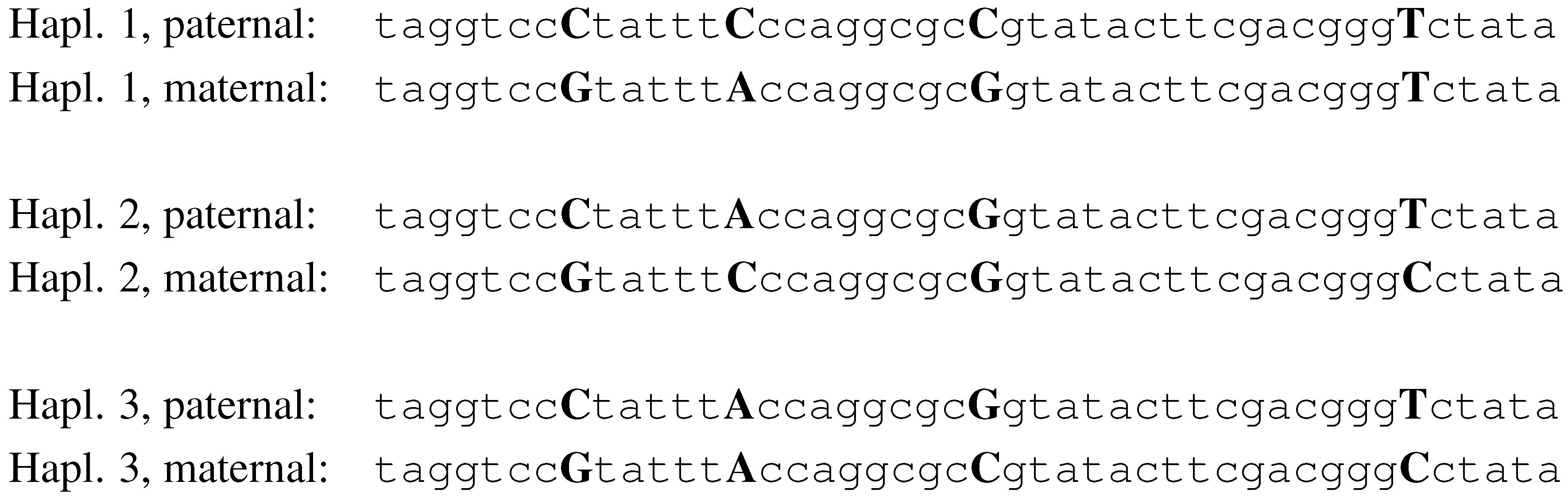
The haplotypes of 3 individuals, with 4 SNPs.
Figure 2.
The haplotypes of 3 individuals, with 4 SNPs.
Gene contents are not the only type of polymorphisms. In fact, any variability in the content of a genomic region within a population is a polymorphism (although it may not be as readily observable as, e.g., the color of a plant’s flowers). The smallest polymorphism at the genome level is the single nucleotide polymorphism (SNP). A SNP is a locus of a specific nucleotide showing a statistically significant variability within a population. Besides very rare exceptions, at each SNP site we observe only two alleles (out of the possible four, A, T, C and G). The recent completion of the sequencing phase of the Human Genome Project has shown the vast majority of polymorphisms in humans are in fact SNPs, occurring, on average, one in each thousand bases.
For a given SNP, an individual can be either homozygous or heterozygous. The values of a set of SNPs on a particular chromosome copy define a
haplotype. In
Fig. 2, we illustrate a simplistic example of three individuals and four SNPs. The alleles for SNP 1, in this example, are C and G. Individual 1, in this example, is heterozygous for SNPs 1, 2 and 3, and homozygous for SNP 4. His haplotypes are
CCCT and
GAGT.
Haplotyping an individual consists of determining his two haplotypes, for a given chromosome. With the larger availability in SNP genomic data, recent years have seen the birth of a set of new computational problems related to haplotyping. These problems are motivated by the fact that it is economically infeasible to determine the haplotypes experimentally. On the other hand, there is a cheap experiment which can determine the (less informative and often ambiguous) genotypes, from which the haplotypes must then be retrieved computationally. A genotype provides, for an individual, information about the multiplicity of each SNP allele: i.e., for each SNP site, the genotype specifies if the individual is heterozygous or homozygous (in the latter case, it also specifies the allele). The ambiguity comes from heterozygous sites, since, to retrieve the haplotypes, one has to decide how to distribute the two allele values on the two chromosome copies (a problem also called phasing the alleles).
Problem area # 4: Haplotyping. Reconstruction and/or correction of haplotypes from partial haplotype fragments or from genotype data. Analysis of resulting haplotypes and correlation with genetic diseases.
Evolution. A branch of genetics known as evolutionary genetics, studies genomic changes that have occurred over long periods of time. For such changes the effects are so dramatic that they give rise to different families within species, or possibly completely new species. The main data structure used to represent evolutionary relationships is the
phylogenetic tree, illustrated in
Figure 3.
Figure 3.
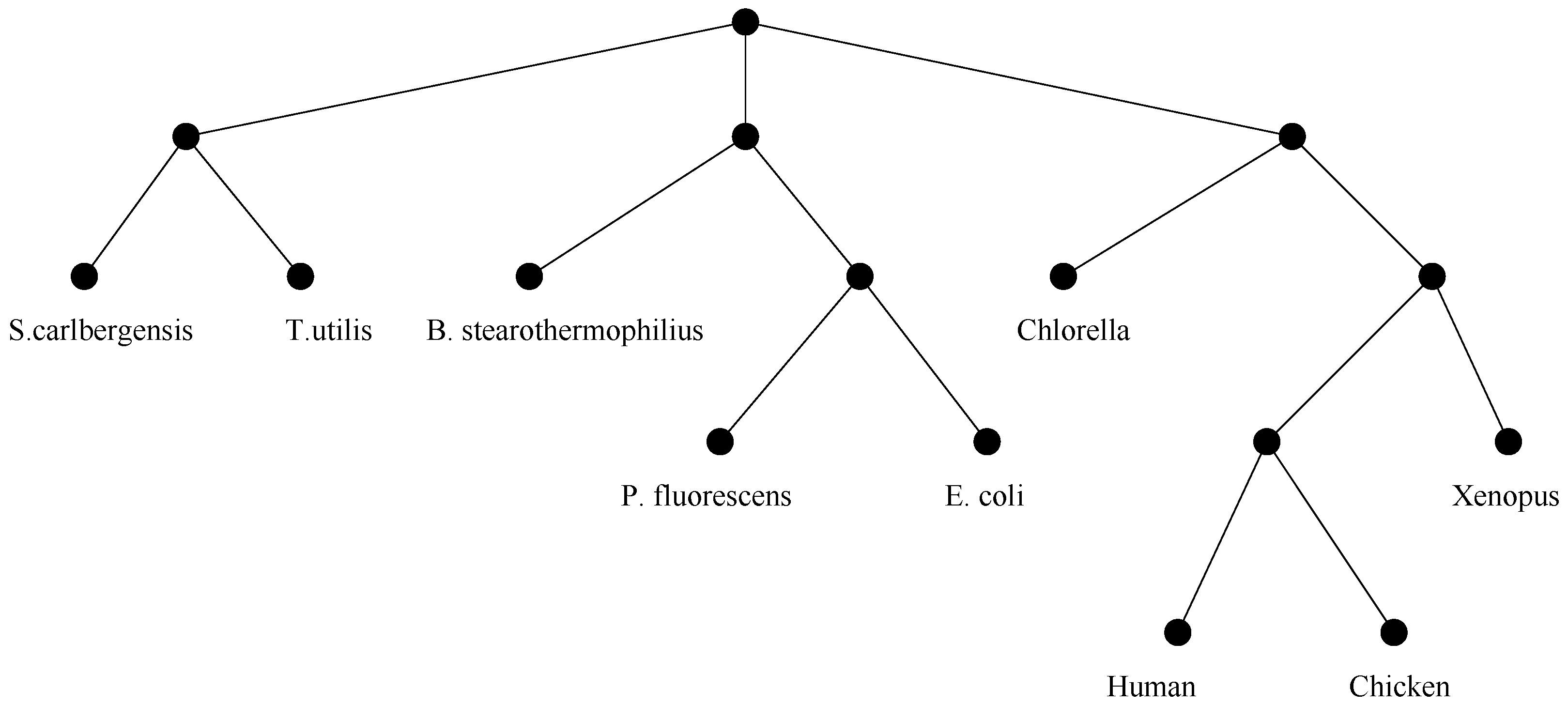
An example of evolutionary tree.
Figure 3.
An example of evolutionary tree.
At each branching point in the tree we associate one or more “evolutionary events” which are mutations in the genome of one species resulting in descendants of new species. An important class of these mutations are the so called
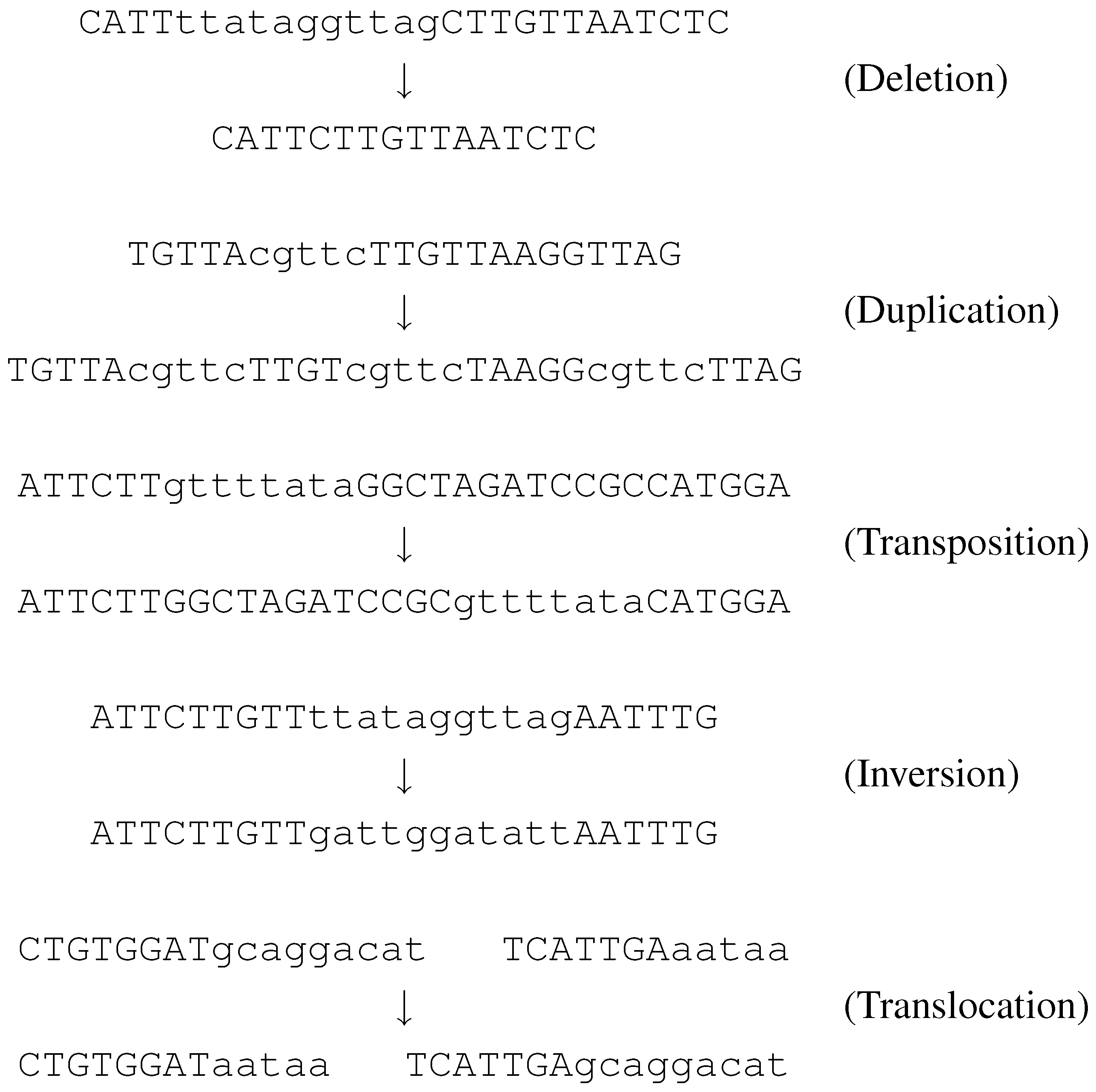
genome rearrangements. These are simply misplacements of large DNA regions, such as deletions, duplications, transpositions, inversions, and translocations. These events affect a long fragment of DNA on a chromosome. In a deletion the fragment is simply removed from the chromosome. A duplication creates many copies of the fragment, and inserts them in different positions, on the same chromosome. When an inversion or a transposition occurs, the fragment is detached from its original position and then is reinserted, on the same chromosome. In an inversion, it is reinserted at the same place, but with opposite orientation than it originally had. In a transposition, it keeps the original orientation but ends up in a different position. Finally, a translocation causes a pair of fragments to be exchanged between the ends of two chromosomes.
Figure 4 illustrates these events, where each string represents a chromosome.
Since evolutionary events affect long DNA regions (several thousand bases), the basic unit for comparison is not the nucleotide, but rather the gene. The computational study of rearrangement problems started after it was observed that several species share the same genes, however differently arranged. For example, most genes of the genome of Brassica oleracea (cabbage) are identical in Brassica campestris (turnip), but appear in a completely different order.
Figure 4.
Five types of evolutionary events
Figure 4.
Five types of evolutionary events
When two whole genomes are compared, the goal is that of finding a sequence of evolutionary events that, applied to the first genome, turn it into the second. Usually, the objective asks to find the most parsimonious set of events, and the solution provides a lower bound on the “amount of evolution” between the two genomes. This bound can be interpreted as an evolutionary distance, and can be used to compute phylogenetic trees over a set of species. Species which are at short evolutionary distance should be placed very close in the tree (i.e., their paths to the root should intersect rather soon at a common ancestor).
Depending on the type of evolutionary distance used, there may be many distinct evolutionary trees over the same set
S of species. When many trees are available, it is important to compare them and to find what they have in common. This problem is called the
tree consensus or
tree reconciliation. A similar problem can be posed also in the opposite direction. That is, given “small” trees over some subsets of
S, find a supertree, over all the species, which best agrees with the input trees. This problem is called
supertree reconstruction. We can then define the last problem area:
Problem area # 5: Evolution. Comparison of whole genomes to highlight evolutionary macro events (inversions, transpositions, translocations). Computation of evolutionary distances between genomes. Computation of common evolutionary subtrees or of evolutionary supertrees.
3. The papers
This section contains an annotated bibliography of mathematical programming papers in computational biology, grouped by problem areas.
The papers employ different types of approaches and can be further characterized according to the approach and the results they achieve. In particular, we will use the following characterization of papers:
- ILP.
Papers in this group use Integer Linear Programming formulation to solve the problem, by Branch-and-Bound, Branch-and-Cut, or Branch-and-Price.
- QSDP.
Papers in this group use either Quadratic Programming or Semidefinite Programming.
- LR.
Papers in this group use Lagrangian Relaxation for solving the problem.
- LP-APPR.
Papers in this group use Linear Programming relaxations and rounding to obtain approximation-guarantee algorithms.
- RED.
Papers in this group reduce a computational biology problem to a standard combinatorial optimization problem, such as TSP, Set Covering or Maximum Independent Set.
- OTH.
Papers in this group use some other form of combinatorial optimization results. For instance, some papers try to find a Maximum Feasible Subset of an LP; other papers use global, non-linear, optimization. Still others use Linear Programming to obtain lower bounds and discuss the effectiveness of some proposed heuristic.
3.1. Problem area # 1 : sequence analysis
Multiple alignment. Comparing genomic sequences drawn from individuals of the same or different species is one of the fundamental problems in molecular biology. The comparisons are aimed at identifying highly conserved (and, therefore, presumably functionally relevant) DNA regions, spot fatal mutations, suggest evolutionary relationships, or help in correcting sequencing errors.
A genomic sequence can be represented as a string over an alphabet Σ consisting of either the 4 nucleotide letters or the 20 letters identifying the 20 aminoacids. Aligning a set of sequences (i.e., computing a Multiple Sequence Alignment) consists in arranging them in a matrix having each sequence in a row. This is obtained by possibly inserting gaps (represented by the ‘-’ character) in each sequence so that they all result of the same length. The goal of identifying common patterns is pursued by attempting as much as possible to place the same character in every column. The following is a simple example of an alignment of the sequences ATTCCGAC, TTCCCTG and ATCCTC. The example highlights that the pattern TCC is common to all sequences.
| A | T | T | C | C | G | A | – | C |
| – | T | T | C | C | C | – | T | G |
| A | – | T | C | C | – | – | T | C |
The multiple sequence alignment problem has been formalized as an optimization problem. The most popular objective function for multiple alignment generalizes ideas from optimally aligning two sequences. This problem, called pairwise alignment, is formulated as follows: Given symmetric costs (or, alternatively, profits) for replacing a letter a with a letter b and costs for deleting or inserting a letter a, find a minimum-cost (respectively, maximum-profit) set of symbol operations that turn a sequence into a sequence . For genomic sequences, the costs are usually specified by some widely used substitution matrices (e.g., PAM and BLOSUM), which score the likelihood of specific letter mutations, deletions and insertions.
An
alignment of two or more sequences is a bidimensional array having the (gapped) sequences as rows. The value
of an alignment of two sequences
and
is obtained by adding-up the costs for the pairs of characters in corresponding positions. The objective is generalized, for
k sequences
, by the
Sum–of–Pairs (SP) score, in which the cost of an alignment is obtained by adding-up the costs of the symbols matched up at the same positions, over all the pairs of sequences:
where
denotes the length of the alignment, i.e., the number of its columns.
Finding the optimal SP alignment was shown to be NP-hard by Wang and Jiang [
4]. A Dynamic Programming solution for the alignment of
k sequences, of length
l, yields an exponential-time algorithm of complexity
. In typical real-life instances, while
k can be possibly small (e.g., around 10),
l is in the order of several hundreds, and the Dynamic Programming approach turns out to be infeasible for all but tiny problems.
Alignment problems can be cast as special types of
non-crossing matching problems. Each sequence
represents the
i-th level of a layered graph, with the letters of
being the nodes of the graph at level
i. Each pair of levels induces a complete bipartite graph. A matching between two levels specifies which characters have to be aligned to each other. The matching must be non-crossing, i.e., if the
k-th letter of a sequence is matched to the
j-th letter of another, no letter preceding
k in the first sequence can be matched to a letter following
j in the second. Furthermore, the union of the non-crossing matchings between each pair of levels must be realizable at the same time by the same multiple alignment of all the sequences. This condition amounts to saying that the union of all the matchings must form a
trace, a concept introduced in 1993 by Kececioglu [
5].
[
6]: J. Kececioglu, H.-P. Lenhof, K. Mehlhorn, P. Mutzel, K. Reinert and M. Vingron (2000) [ILP]
study a Branch-and-Cut approach for the the Maximum Weight Trace (MWT) Problem. The MWT generalizes the SP objective as well as many other alignment problems in the literature. Some polyhedral results are presented characterizing the facets of the polyhedron of feasible solutions. The algorithm is used to optimally align 15 proteins of length about 300 each.
The polyhedral study of the trace polytope, together with the introduction of new classes of valid inequalities and corresponding separation algorithms is further pursued in
[
7]: E. Althaus, A. Caprara, H.-P. Lenhof and K. Reinert (2006) [ILP]
The inverse multiple alignment problem starts from a set of “good” alignments (e.g., validated by the biologists) and aims at determining a cost function, in the form of substitution matrix and gap penalties, under which the given alignments are optimal. This problem is studied by
[
8]: J. Kececioglu and E. Kim (2006) [ILP]
and an integer programming formulation is proposed for its solution.
[
9]: M. Fischetti, G. Lancia and P. Serafini (2002) [RED,ILP]
reduce the multiple alignment problem to the minimum routing cost tree (MRCT) problem, i.e., finding a spanning tree in a complete weighted graph, which minimizes the sum of the distances between each pair of nodes. They propose a Branch-and-Price algorithm for the MRCT problem and then use it to align up to 30 protein sequences of several hundred letters each.
[
10]: W. Just and G. Della Vedova (2004) [RED]
reduce multiple sequence alignment to a facility location problem. The reduction is then used to provide a Polynomial Time Approximation Scheme for a certain class of multiple alignment problems. Moreover, it is shown that optimizing the Sum-of-Pairs objective function is APX-hard.
Sequence alignment is often used to retrieve all sequences similar to a given query from a genomic database. In order to speed-up the search, one strategy is to map the sequences into a binary space in such a way that the Hamming distance between strings is comparable to the similarity of the original sequences.
[
11]: E. Boros and L. Everett (2005) [ILP]
employ linear programming techniques to model and study the nature of mapping schemes from protein sequences into binary vectors. The objective is to minimize the distortion between edit distance and Hamming distance. The work achieves the theoretically minimum distortion for several biological substitution matrices.
Consensus sequence. Given a set S of sequences, an important problem requires to determine their consensus, i.e., a sequence which somewhat represents all the sequences in the set. This sequence is defined as the sequence which minimizes . Another definition of consensus, which is used when the set S is biased towards some subset of sequences (e.g., human sequences vs other species), is the sequence which minimizes . This sequence is also called the closest sequence to S. Similarly, the farthest sequence is the sequence which maximizes . The closest sequence problem is studied in
[
12]: C. Meneses, Z. Lu, C. Oliveira and P. Pardalos (2004) [ILP]
where three integer programming formulations are proposed for its solution. The best formulation is used for solving problems with up to 30 sequences of length 700 each. A similar formulation is used by
[
13]: A. Ben-Dor, G. Lancia, J. Perone and R. Ravi (1997) [LP-APPR]
for obtaining an approximation algorithm, via the randomized-rounding of the optimal LP-relaxation solution.
The rounding of LP-relaxation solutions is also used by the following papers to obtain an approximation algorithm (in the form of a Polynomial Time Approximation Scheme) for both the consensus problem and the farthest sequence problem:
[
14]: J. Lanctot, M. Li, B. Ma, S. Wang and L. Zhang (1999) [LP-APPR]
[
15]: M. Li, B. Ma and L. Wang (2002) [LP-APPR]
[
16]: X. Deng, G. Li, Z. Li, B. Ma and L. Wang (2003) [LP-APPR]
Sequence assembly. Integer programming formulations have been used also in the context of sequence assembly, i.e., the process of reconstructing a long DNA sequence by the merging of short, overlapping, DNA fragments.
[
17]: J. D. Kececioglu and J. Yu (2001) [ILP]
focuses on the problem of correctly assembling the fragments when repeats are present. Repeats are distinct DNA regions of identical content, and their presence baffles most assembly algorithms. In fact, fragments coming from distinct repeats, having perfect ovelap, tend to be merged together into one single copy of the repeat. The approach followed here is to formulate the problem of correcting a wrong assembly, in the presence of repeats, as an integer linear programming problem, solved by Branch-and-Bound.
[
18]: C. E. Ferreira, C. C. de Souza and Y. Wakabayashi (2002) [ILP]
also consider the problem of assembling DNA fragments to reconstruct an original target sequence. The focus in this paper is on the possibility that gaps are present, and so the reconstruction should not build only one sequence (called contig), but perhaps many. The objective is to reconstruct the smallest number of contigs such that each fragment is covered by one contig, and each contig is obtained by chaining some fragments, , such that the last l characters (for some l) are identical to the first l characters of . This problem is formulated by integer programming, and solved by Branch-and-Cut.
Motif finding is still another type of sequence analysis problem. This problem consists in the study of a set of sequences, in order to identify recurring patterns (motifs) that are present -modulo small mutations- in all sequences. This problem is reduced to a graph problem, solved by integer programming, in the following works:
[
19]: C. Kingsford, E. Zaslavsky, and M. Singh (2006) [RED,ILP]
[
20]: E. Zaslavsky and M. Singh (2006) [RED,ILP]
3.2. Problem area # 2 : hybridization and microarrays
Physical mapping. Physical mapping by hybridization is the problem of reconstructing the linear ordering of a set of genetic markers, called probes, along a target (such as a BAC, Bacterial Artificial Chromosome). The input of this problem usually consists of a probe/clone 0-1 incidence matrix, i.e., a matrix specifying, for each pair (probe, clone), if the probe is contained in the clone.
[
21]: F. Alizadeh, R. Karp and L. Newberg and D. Weisser (1995) [RED]
show how to cast this problem into a special type of TSP, the Hamming distance TSP, which is then solved by the use of standard TSP heuristics.
A very similar problem concerns the construction of Radiation Hybrid (RH) maps. Radiation hybrids are obtained by (i) breaking, by radiation, a human chromosome into several random fragments (the markers) and (ii) fusing the radiated cells with rodent normal cells. The resulting hybrid cells, may retain one, none or many of the fragments from step (i). For each marker j and each radiation hybrid i, an experiment can tell if j was retained by i or not. As before, the problem consists in ordering the markers, given M. The problem is studied in
[
22]: A. Ben-Dor and B. Chor (1997) [RED]
[
23]: A. Ben-Dor and B. Chor and D. Pelleg (2000) [RED]
Two different measures are widely used to evaluate the quality of a solution. The first is a combinatorial measure, called Obligate Chromosome Breaks (OCB), while the second is a statistically based, parametric method of maximum likelihood estimation (MLE). The optimization of both measures can be reduced to the solution of a suitable TSP. In their work, Ben Dor at al. used
Simulated Annealing, with the 2-OPT neighborhood structure of Lin and Kernighan [
24], for the solution of the TSP.
The software package RHO (Radiation Hybrid Optimization), developed by Ben Dor et al., was used to compute RH maps for the 23 human chromosomes. For 18 out of 23 chromosomes, the maps computed with RHO coincided with the corresponding maps computed at the Whitehead Institute, by experimental, biological, techniques. The remaining maps computed by using RHO were superior to the Whitehead maps with respect to both optimization criteria.
[
25]: R. Agarwala, D. Applegate, D. Maglott, G. Schuler, A. Schaffer (2000) [RED]
describe an improvement of the RHO program, obtained by replacing the simulated annealing module for the TSP with the state-of-the-art TSP software package, CONCORDE [
26]. Computational experiments showed that the maps computed by the program over hybrid data from the panels Genebridge 4 and Stanford G3, were more accurate than the previously known maps over the same data.
The physical mapping problem has been attacked also by integer programming formulations, solved via Branch-and-Cut.
[
27]: T. Christof, M. Junger, J. Kececioglu, P. Mutzel and G. Reinelt (1997) [ILP]
[
28]: T. Christof and J. D. Kececioglu (1999) [ILP]
The second of these works, in particular, focuses on physical mapping with end-probes, in which the probes used for hybridization come in pairs. Each pair consists of two short sequences flanking the ends of some longer clone.
Microarrays and feature selection. Hybridization is at the basis of microarrays technology. A microarray is a matrix in which each cell is labeled with some probe. Microarraye experiments (heavily parallel as the number of cells in a microarray is typically quite large), can tell which subset of the probes hybridize to the sample. The characteristic vector of the subset can then be used as a signature for the sample, as long as no other sample has the same characteristic vector. The problem of selecting probes which yield “good” signatures for a set of samples is solved by integer programming in
[
29]: G. W. Klau, S. Rahmann, A. Schliep, M. Vingron and K. Reinert (2004) [ILP]
The above problem belongs to the general class of
feature selection problems. The incidence of a probe to a target can be seen as a feature that the target may or may not possess. The signatures can be used to classify a set of targets (e.g., tissues), as long as, for each pair of tissues, there is at least one feature possessed by one tissue but not by the other. Approximation algorithms for the tissue classification problem, reduced to the
minimum test collection problem (problem SP6 in [
30]), are studied in
[
31]: K. M. De Bontridder, B. Halldorsson, M. Halldorsson, C. A. J. Hurkens, J. K. Lenstra, R. Ravi and L. Stougie (2003) [RED]
Tissue classification via microarray experiments has been also studied in relation to the treatment and diagnosis of various forms of cancers. The problem here is that of finding a set of features that can discriminate healthy tissues from diseased ones, and hence, that can be associated to the disease. This clustering problem is solved with the use of both linear programming and non linear optimization in
[
32]: K. Munagala, R. Tibshirani and P. O Brown (2004) [OTH]
and in
[
33]: R. Berretta, A. Mendes and P. Moscato (2005) [OTH,ILP]
[
34]: P. Moscato, R. Berretta, A. Mendes, M. Hourani and C. Cotta (2005) [OTH,ILP]
Similarly, linear programming solutions to clustering problems for a general feature selection problem are used in
[
35]: C. Bhattacharyya, L. R. Grate, A. Rizki, D. Radisky, F. J. Molina, M. I. Jordan, M. J. Bissell and I. S. Mian (2003) [OTH]
PCR primers and SBH. The primer selection problem for PCR experiments is usually solved by a reduction to the Set Covering problem. Such an approach is present in
[
36]: W. R. Pearson, G. Robins, D. E. Wrege and T. Zhang (1996) [RED]
[
37]: P. Nicodeme and J. M. Steyaert (1997) [RED]
Hybridization is finally used for DNA sequencing, in the recent technique called “sequencing by hybridization” (SBH). SBH is a sequencing method that uses DNA chips to reconstruct a DNA sequence from fragmental subsequences. When the experimental data are error-free, the problem of reconstructing the original DNA sequence reduces to the Eulerian path problem, for which linear-time algorithms are known. However, the same problem is NP-hard for data containing errors.
[
38]: Y. J. Chang and N. Sahinidis (2005) [ILP]
formulate the SBH problem as a mixed-integer linear program with an exponential number of constraints. A separation algorithm is developed to solve the model. The proposed approach is used to solve large SBH problems to global optimality efficiently.
3.3. Problem area # 3: protein structure
Protein folding. The protein folding problem consists in computing the native fold of a protein from either its aminoacid sequence alone, or from the sequence and a library of known folds. The former case is called the folding ab-initio problem, while the latter is called threading. In both cases, the optimal fold sought after should minimize the free energy of the structure. Unfortunately, there is no simple-to-handle formula for the free energy. One of the main questions studied today is that of approximating the protein energy by a suitable, simpler, function, such as a linear function whose contributions are some pairwise weights which depend on (the interaction forces between) pairs of aminoacids. This problem is studied, e.g., in
[
39]: M. Wagner, J. Meller and R. Elber (2004) [OTH]
where it is solved as an inverse optimization problem: starting from the optimal solutions (known protein folds, determined experimentally) try to infer a function which is optimized by these solutions and not by others. The problem is cast as a linear program. Since this is only an approximation, and it may happen that the LP is infeasible, the authors reduce the energy determination problem to a max feasible subsystem problem.
Folding prediction ab-initio is a very difficult problem. A typical simplification, although still hard to solve, is to consider each aminoacid as one of two types: H, i.e, hydrophobic, or P, i.e., hydrophilic (also called polar). A protein is then a string over . Furthermore, the folding angles are restricted to some set of discrete possibilities (e.g., 90 degrees only) and therefore the aminoacids have to be placed over the vertices of a 3D square lattice, following a so-called self-avoiding walk. The objective function is that of placing in adjacent vertices of the lattice as many hydrophobic aminoacids as possible. This is called the HP model of protein folding.
[
40,
41]: R. Carr, W. Hart and A. Newman (2002,2004) [ILP]
propose integer linear programming approaches for the solution of the HP protein folding problem. It should be said that the ILP approach for this problem has not proved to be as effective as other solution methods. The ILP fails to find optimal folds for proteins longer than 30 aminoacids. The most successful approaches for HP folding are based on constraint programming, a technique that allows the optimal solution for instances of up to 200 aminoacids [
42].
A much better success has been met by integer programming approaches for the protein threading problem. In particular, RAPTOR, a computer program implementing a Branch-and-Cut formulation for threading, has won the fully-automated fold prediction contest CAFASP.
[
43]: J. Xu, M. Li, D. Kim and Y. Xu (2003) [ILP]
[
44]: J. Xu and M. Li (2003) [ILP]
[
45]: J. Xu and M. Li and Y. Xu (2004) [ILP]
A parallelization of the ILP approach for protein threading has been studied in
[
46]: R. Andonov and S. Balev and N. Yanev (2004) [OTH]
Both an integer programming formulation and a Lagrangian-relaxation approach for threading are proposed in
[
47]: P.Veber, N. Yanev, R. Andonov and V. Poirriez (2005) [ILP,LR]
Furthermore, threading has been successfully approached also by global, non-linear optimization algorithms. The approach described in
[
48]: E. Eskow, B. Bader, R. Byrd, S. Crivelli, T. Head-Gordon, V. Lamberti and R. Schnabel (2004) [OTH]
was used to predict the fold of proteins of up to 4000 aminoacids.
Protein design. In the protein design problem, the objective is to determine a protein (i.e., an aminoacid sequence) that folds into a target structure. In a variant of the protein design problem, only part of the structure is fixed (the protein’s backbone), while the rest of the structure, in the form of its side-chains), has to be chosen optimally from a library of side-chains conformations.
[
49]: S. K. Koh and G. K. Ananthasuresh and C. Croke (2004) [OTH]
[
50]: S. K. Koh, G. K. Ananthasuresh, S. Vishveshwara (2005) [OTH]
describe a quadratic optimization problem for protein design in the HP model. The problem is solved by gradient-based mathematical programming techniques.
Integer programming formulations for the side-chain positioning problem have been described in
[
51]: O. Eriksson, Y. Zhou and A. Elofsson (2001) [ILP]
[
52]: C. Kingsford and B. Chazelle and M. Singh (2005) [ILP]
In the latter work, the LP relaxation of the integer programming formulation is used to obtain a polynomial-time LP-based heuristic. Computational experiments show that the LP-based solutions are oftentimes optimal. The same authors investigate a quadratic programming formulation for the problem, solved by semidefinite programming, in
[
53]: B. Chazelle, C. Kingsford and M. Singh (2004) [QSDP]
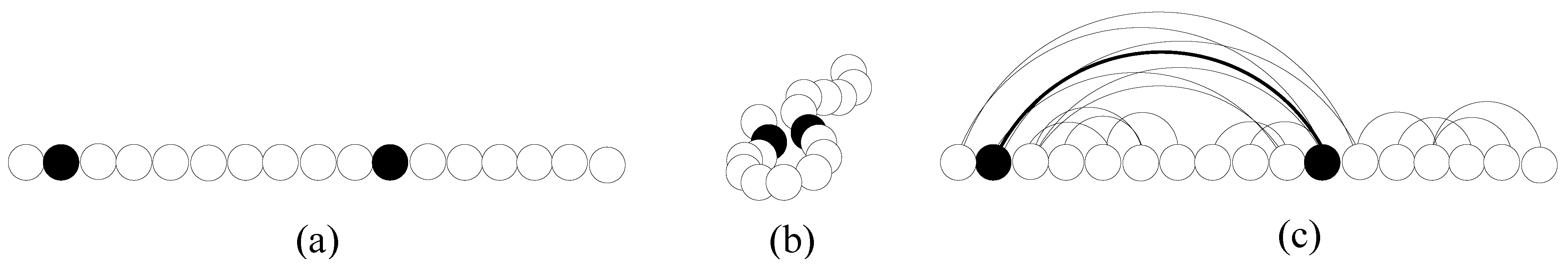
Figure 5.
(a) An unfolded protein. (b) After folding. (c) The contact map graph.
Figure 5.
(a) An unfolded protein. (b) After folding. (c) The contact map graph.
Protein docking. The docking problem for protein structures consists in (i) predicting the way in which some 3D structures interact geometrically, or (ii) designing 3D structures that will bind (dock) with some known target 3D structures. A Branch-and-Cut approach for docking is proposed in
[
54]: E. Althaus and O. Kohlbacher and H.-P. Lenhof and P. Muller (2002) [ILP]
The problem solved in this work is similar to the side-chain positioning problem. Given two structures, their interaction can be seen as the sum of a “rigid” part, given by the interaction of their backbones, plus a “flexible” part, given by the best placement for the set of their side-chains. The authors show that the key in solving the docking problem lies in the ability of computing the best possible side-chain placement, which they formulate as an integer programming problem.
Global optimization approaches for both folding and docking problems are described in
[
55]: C. Floudas and J. Klepeis and P. Pardalos (1998) [OTH]
(see also [
56] for a survey on global optimization in molecular biology).
Structure alignment. An alignment of two (or more) protein structures is a mapping which sets a correspondence between similar structural elements in the two proteins. An alignment can be either global or local. In the former case, the optimal alignment should maximize the total similarity of the corresponding elements, over the entire structures. In the latter case, the goal is to find a (sufficiently large) sub-structure which is very similar in the two targets.
The score of an alignment is a numerical measure of the similarity between the two structures. One scoring function that has received a great deal of attention in the past few years is the contact map overlap (CMO) measure.
When the protein folds to its native, two aminoacids that are distant in the sequence may end up in close proximity in the fold (see
Figure 5 (a) and (b)). If the distance between two aminoacids in the fold is smaller than a certain threshold (e.g., 5 Å), then the aminoacids are said to be
in contact. The
contact map for a protein is a graph, whose vertices are the aminoacids of the protein, and whose edges connect each pair of aminoacids in contact (see
Figure 5 (c)).
The CMO tries to evaluate the similarity in the 3-D folds of two proteins by determining the similarity of their contact maps (the rationale being that a high contact map similarity is a good indicator of high 3-D similarity). Given two folded proteins, the CMO problem calls for determining an alignment between the aminoacids of the first protein and of the second protein. The alignment specifies the aminoacids that are considered equivalent in the two proteins. The value of an alignment is given by the number of pairs of aminoacids in contact in the first protein which are aligned with pairs of aminoacids that are also in contact in the second protein. The goal is to find an alignment of maximum score.
[
57,
58,
59]: A. Caprara, B. Carr, S. Istrail, G. Lancia and B. Walenz (2001,2002,2004) [ILP,LR]
describe an integer programming formulation of the CMO problem, and a Branch-and-Cut approach for its solution. Furthermore, a Lagrangian relaxation approach is described which starts from a quadratic programming formulation of the problem. The Lagrangian relaxation approach turns out to be very effective, allowing the optimal solution of real proteins from the PDB (Protein Data Bank) with up to a few hundred aminoacids.
[
60]: R. Carr and G. Lancia (2004) [OTH]
show how the integer programming formulation of the problem can be cast as a compact optimization model, in which the exponential number of inequalities (added via separation algorithms during the Branch-and-Cut search), are replaced by a polynomial number of new inequalities and variables. The compact model turns out to be up to two orders of magnitude faster to solve than the original ILP.
The CMO problem can be reduced to a maximum-weight clique problem on a very special type of layered graph (a grid graph, with vertices for and and edges for each pair such that and ). The special nature of the graph is exploited for a fast max-weight clique algorithm in
[
61]: E. Barnes and J. S. Sokol and D. M. Strickland (2005) [RED]
The Lagrangian relaxation approach which has proved successful for CMO is used for the multiple alignment of RNA secondary structures in
[
62]: M. Bauer and G. W. Klau (2004) [LR]
[
63]: M. Bauer, G. W. Klau and K. Reinert (2005) [LR]
3.4. Problem area # 4 : haplotyping
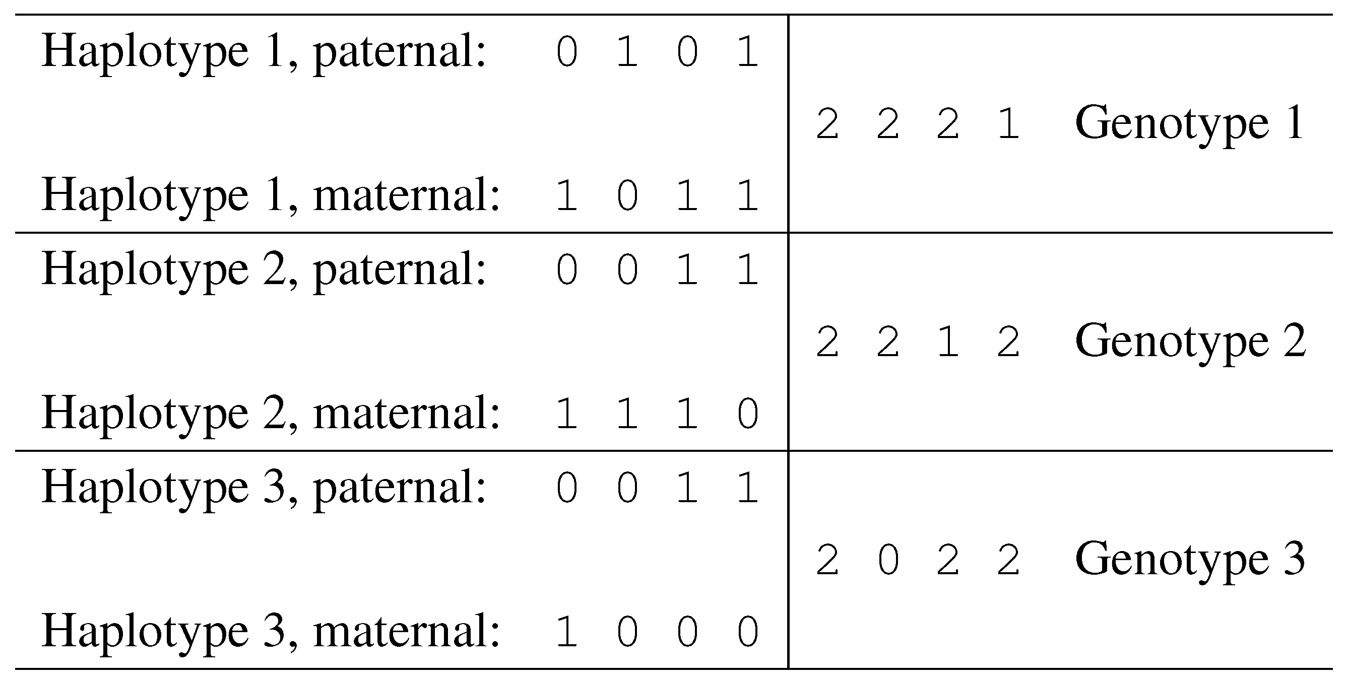
Notation. Given a set of n SNPs, fix a binary encoding of the two alleles for each SNP (e.g., call “0” the least frequent allele and “1” the most frequent allele). With this encoding, each haplotype corresponds to binary vector of length n.
Given two haplotypes
and
, define their sum as a vector
, of length
n, and with components in
. The vector
g is called a genotype, and its components are defined as follows:
Each position
i such that
is called an
ambiguous position. Genotype entries of value 0 or 1 correspond to homozygous SNP sites, while entries of value 2 correspond to heterozygous sites. In
Fig. 6 we illustrate a case of three individuals, showing their haplotypes and genotypes.
Figure 6.
Haplotypes and corresponding genotypes.
Figure 6.
Haplotypes and corresponding genotypes.
A resolution of a genotype g is a pair of haplotypes and such that . The haplotypes and are said to resolve g. A genotype is ambiguous if it has more than one possible resolution, i.e., if it has at least two ambiguous positions. A haplotype h is said to be compatible with a genotype g if h can be used in a resolution of g. Two genotypes g and are compatible if there exists at least one haplotype compatible with both of them, otherwise, they are incompatible.
For the haplotyping problems described in this section, the input data consist in a set of m genotypes , corresponding to m individuals in a population. The output is set of haplotypes such that, for each , there is at least one pair of haplotypes , with . The set of is said to explain .
Clark’s rule. The first haplotyping problem studied was related to the optimization of
Clark’s inference rule (IR). The rule, proposed by the geneticist Clark [
64], can be used to resolve a genotype
g whenever a haplotype
h compatible with
g is known. The rule derives new haplotypes by inference from known ones as follows:
- IR:
Given a genotype g and a compatible haplotype h, obtain a new haplotype q by setting at each ambiguous position j and at the remaining positions. Then h and q resolve g.
In order to resolve all genotypes, Clark suggested the use of successive applications of the inference rule, starting from a “bootstrap” set of known available haplotypes. In essence, Clark proposed the following algorithm: (i) take an unsolved genotype g and an available compatible haplotype h; (ii) derive q by inference, and solve g as ; (iii) declare g solved and q available. If there are still unsolved genotypes go to (i).
If at the end all genotypes have been solved, the algorithm succeeds, otherwise, it fails (this happens if in step (i) there are no compatible available haplotypes for an unsolved genotype). Notice that the procedure, as outlined, is nondeterministic since it does not specify how to choose the pair whenever there are more candidates to the application of the rule. It can be shown that, because of this vagueness, there may be two runs of the algorithm on the same data such as one run succeeds while the other fails.
[
65]: D. Gusfield (2001) [RED,ILP]
studies the problem of finding an optimal order of application of Clark’s rule. The objective is that of leaving the fewest number of unsolved genotypes in the end. The problem is proved to be APX-hard. The solving algorithm consists in first transforming the problem into a maximum weighted forest on a suitable auxiliary graph, and then solving this graph problem by integer programming.
Max parsimony. Since Clark’s algorithm tries to re-use existing haplotypes and to introduce at most one new haplotype at a time, the solution it tends to produce is usually of small size. The objective of minimizing the size of has several biological motivations. For one, the number of distinct haplotypes observed in nature is vastly smaller than the number of possible haplotypes (we all descend from a small number of ancestors, whose haplotypes, modulo some recombination events and mutations, are the same we possess today). Moreover, under a general parsimony principle (also known as Okkam’s razor), of many possible explanations of an observed phenomenon, one should favor the simplest.
The pure parsimony haplotyping problem requires to find a solving set of smallest possible cardinality. This problem has been introduced by Gusfield
[
66]: D. Gusfield (2003) [ILP]
who adopted an integer programming formulation, with an exponential number of variables and constraints, for its practical solution. The ILP approach is shown to be applicable to instances of about 50 genotypes over 30 SNPs, with relatively few (about 10) ambiguous positions per genotype. An alternative, polynomial-size, integer programming formulation is proposed in
[
67]: D. G. Brown and J. M. Harrower (2004) [ILP]
The polynomial-size ILP can be used for some instances which are too large for the exponential model. However, the LP-relaxation bound is weak and the solving process can be quite long. A similar polynomial-size formulation is present also in
[
68]: G. Lancia, C. Pinotti and R. Rizzi (2004) [LP-APPR]
where Gusfield’s exponential model is used to derive an LP-based approximation algorithm, yielding -approximate solutions for instances in which each genotype has at most k ambiguous positions.
[
69]: G. Lancia and R. Rizzi (2006) [ILP,OTH]
prove that the parsimony problem for instances in which each genotype has at most two ambiguous positions is polynomially solvable. The proof consists in showing that, in this special case, the solution of the ILP is naturally integer.
The pure parsimony haplotyping problem has also been formulated as a quadratic problem.
[
70]: K. Kalpakis and P. Namjoshi (2005) [QSDP]
use semidefinite programming for its solution. Similarly to the exponential IP, the formulation has a variable for each possible haplotype and cannot be used to tackle instances for which the set of possible haplotypes is too large. The size of the problems solved is about the same as for the previous methods. Based on a similar formulation, an (exponential-time) approximation algorithm is presented in
[
71]: Y.T. Huang, K.M. Chao and T. Chen (2005) [QSDP]
Families and disease association. When collecting genotype data for populations, sometimes extra information are gathered as well. For instance, information about which individuals of the population are related (i.e., belong to the same family). Furthermore, some individuals may be affected by a genetic disease, so that the genotypes can be labeled as healthy and diseased. When these extra data are available, new combinatorial models can be defined for several problems.
[
72]: D. Brinza, J. He, W. Mao and A. Zelikovsky (2005) [ILP]
In this paper the set of input genotypes is partitioned into family trios, where each trio is composed by a pair of parents and a child. The goal is that of retrieving haplotypes, so that each trio’s genotypes are explained by a quartet of parent/offspring haplotypes. The objectives studied are pure parsimony and missing data recovery. For both problems, the authors propose integer linear programming approaches. The approaches are validated by extensive experiments, showing an advantage in the use of the ILP approach over the previously known methods.
In a similar problem, a set of incomplete genotypes (i.e., with missing alleles) is given, together with a pedigree, i.e., a set of relationships between the genotypes in the form of “the genotype is a descendant of the genotype ”. The objective is that of retrieving pairs of complete haplotypes for all the individuals in the population.
[
73]: J. Li and T. Jiang (2004) [ILP]
show that the problem is NP-hard and give an integer programming formulation, solved via Branch-and-Bound. Computational results show that the method can recover haplotypes with 50 loci from a pedigree of size 30 in a matter of seconds on a standard PC. Its accuracy, in terms of correctly recovered haplotypes, is more than 99.8% for data with no missing alleles and 98.3% for data with 20% missing alleles.
[
74]: W. Mao, J.He, D. Brinza and A. Zelikovsky (2005) [OTH]
focus on the problem of determining if an individual with given genotype is susceptible to develop a certain disease. In order to make this prediction, two sets of genotypes are available in input: a set of healthy genotypes and a set of diseased genotypes. The authors show how to cast the prediction problem as a Linear Program, and validate their approach by several experiments on real data sets.
3.5. Problem area # 5 : evolution
Genome rearrangements. The most common type of genomic rearrangement event is by far the inversion, also called
reversal. A
reversal , with
, is a permutation defined as
If we represent a genome of n genes as a permutation of the numbers , by applying (multiplying) to π, one obtains , i.e., the order of the elements has been reversed.
Given two genomes
π and
σ over the same
n genes, their
reversal distance is the smallest number
d such that there exits reversals
with
Without loss of generality, we can always assume that , so that the problem becomes that of finding the smallest number of reversals that sort a given permutation π. This problem is also known as sorting by reversals (SBR).
[
75]: A. Caprara and G. Lancia and S.K. Ng (1999) [RED,ILP]
describe a column-generation approach for SBR. The approach is based on the solution of a graph problem strictly related to SBR. Each permutation π defines a breakpoint graph , in which the edges are colored red and blue, and the number of red and blue edges incident on any node is the same. The edges of can be decomposed into a set of cycles alternating red and blue edges (called alternating cycles). It can be shown that, to find the optimal solution of SBR, one has to decompose the edges of into the maximum number of alternating cycles. The paper formulates the cycle decomposition problem as an integer programming model with a variable for each alternating cycle. The variables are priced-in via the solution of minimum weighted perfect matching problems. The algorithm is capable of sorting permutations of up to elements in a matter of seconds.
[
76]: A. Caprara and G. Lancia and S.K. Ng (2001) [RED,ILP]
show that, by relaxing the set of variables to the set of pseudo-alternating cycles (i.e., alternating cycles that can re-use some of the edges), the pricing problem becomes matching on bipartite graphs. This is much faster to solve than matching on general graphs. The resulting algorithm is capable of sorting permutations of up to elements in a matter of seconds.
Given permutations , their reversal median is a permutation σ such that the sum of the reversal distance from σ to each of the is minimum.
[
77]: A. Caprara (2003) [RED]
shows how to reduce the reversal median problem to finding a perfect matching in a graph that forms the maximum number of cycles jointly with q given perfect matchings. The paper proposes effective algorithms for its exact and heuristic solution, validated by the solution of a few hundred instances associated with real-life genomes.
Phylogeny reconstruction. Given a set of genomes, one basic problem is that of constructing a phylogenetic tree over the genomes which describes their evolution. The internal nodes of the tree represent ancestral genomes, while the input genomes label the tree leaves. The tree edges are weighted, where the length of each edge is the evolutionary distance (e.g., reversal distance) between the genomes corresponding to the endpoints of the edge. The objective is that of finding the tree of smallest total length. As a by-product, for each pair of input genomes, the total length of the path between them in the tree should approximate their evolutionary distance.
[
78]: J. Tang and B. Moret (2005) [OTH]
describe a linear program whose solution yields a lower bound to the phylogeny reconstruction problem. The LP bound is strong and is used for an effective Branch-and-Bound scheme within GRAPPA, the software suite for genome comparisons.
Supertree methods are used to construct a large tree over a large set of taxa, from a set of small trees over overlapping subsets of the complete taxa set. Typically, the small trees are either triples, i.e., rooted trees over three leaves, or quartets, i.e., unrooted trees over four leaves.
[
79]: S. Snir and Satish Rao (2006) [RED,QSDP]
[
80]: S. Moran, S. Rao and S. Snir (2005) [RED,QSDP]
deal with the supertree reconstruction problem for both triples and quartets. The objective is to build a supertree which agrees with as many triples (quartets) as possible. The authors solve the problem by a divide and conquer approach, in which the divide step is a max cut over a graph representing the triples (quartets) inconsistencies. The max cut is solved by a semidefinite programming-like heuristic that leads to very fast running times.
