
Discrete Element Damage Constitutive Model of Loess and Corresponding Parameter Sensitivity Analysis Based on the Bond Rate

Abstract
1. Introduction
2. Methodology
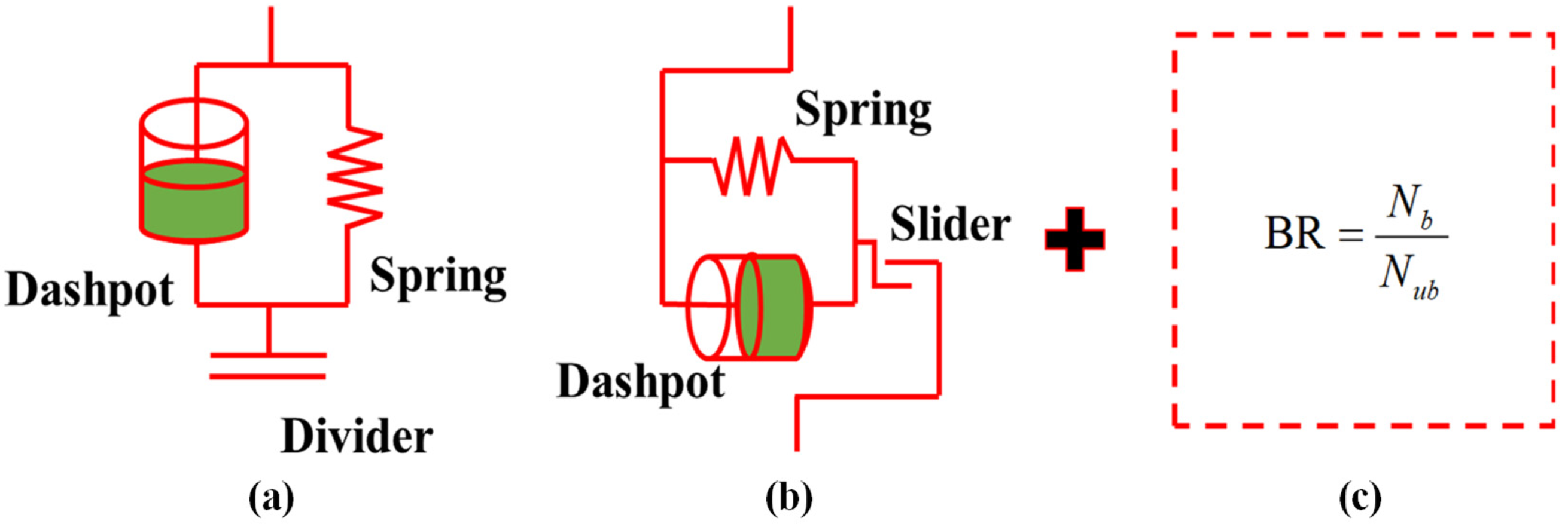
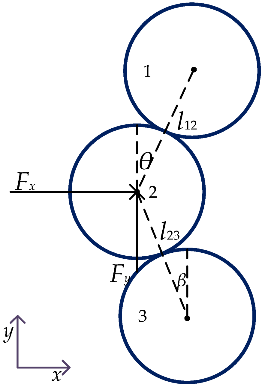
2.1. Discrete Element Damage Constitutive Model Based on the Bond Rate
- (1)
- Stiffness
- (2)
- Strength
- (3)
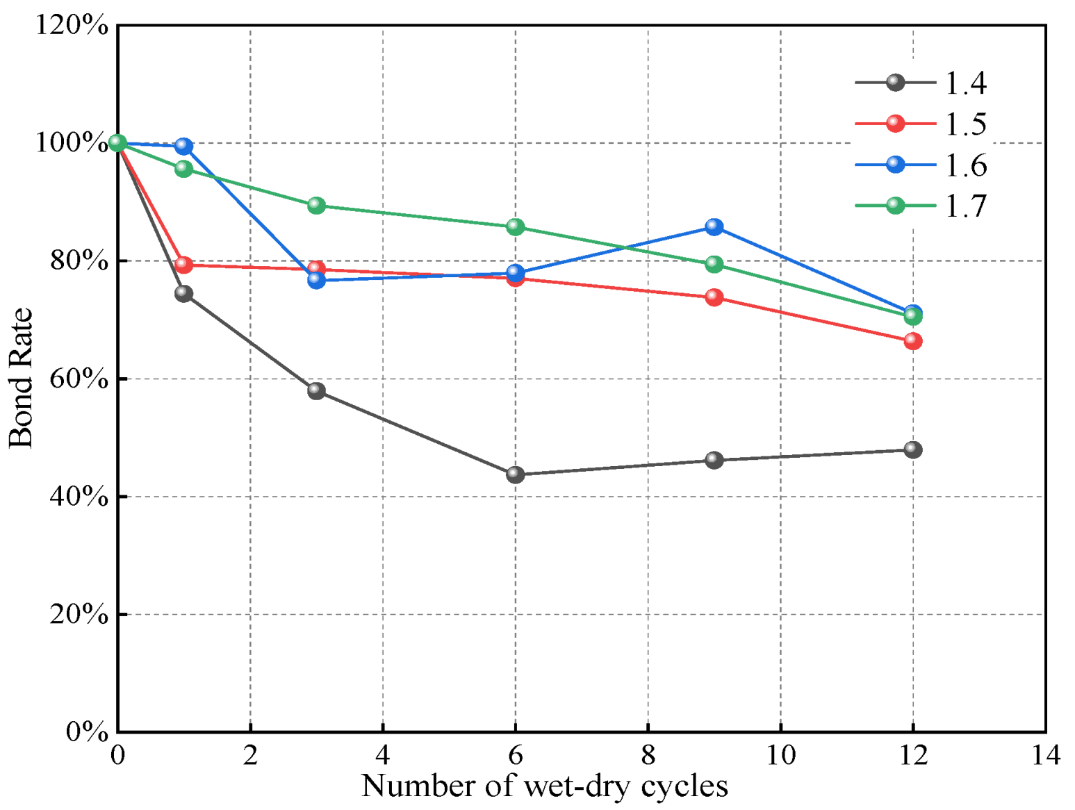
- Bond rate
2.2. Model Building and Solution Process
2.2.1. Specimen Modeling
2.2.2. Boundary Conditions and Servo Control
2.2.3. Loading Process and Solution Procedure
3. Analysis of Microscopic Parameters
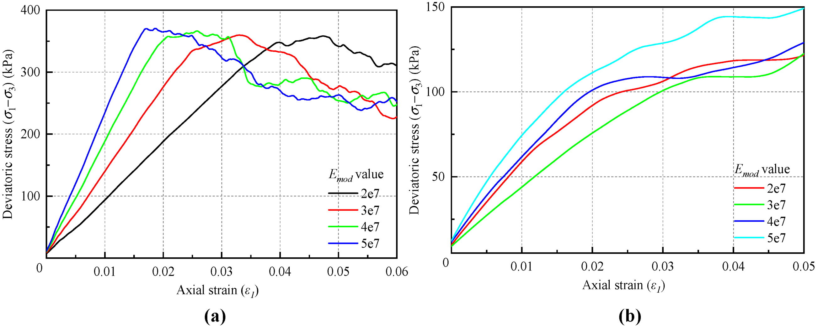
3.1. Contact Stiffness
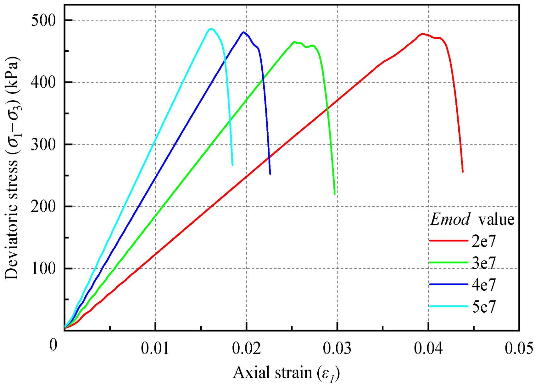
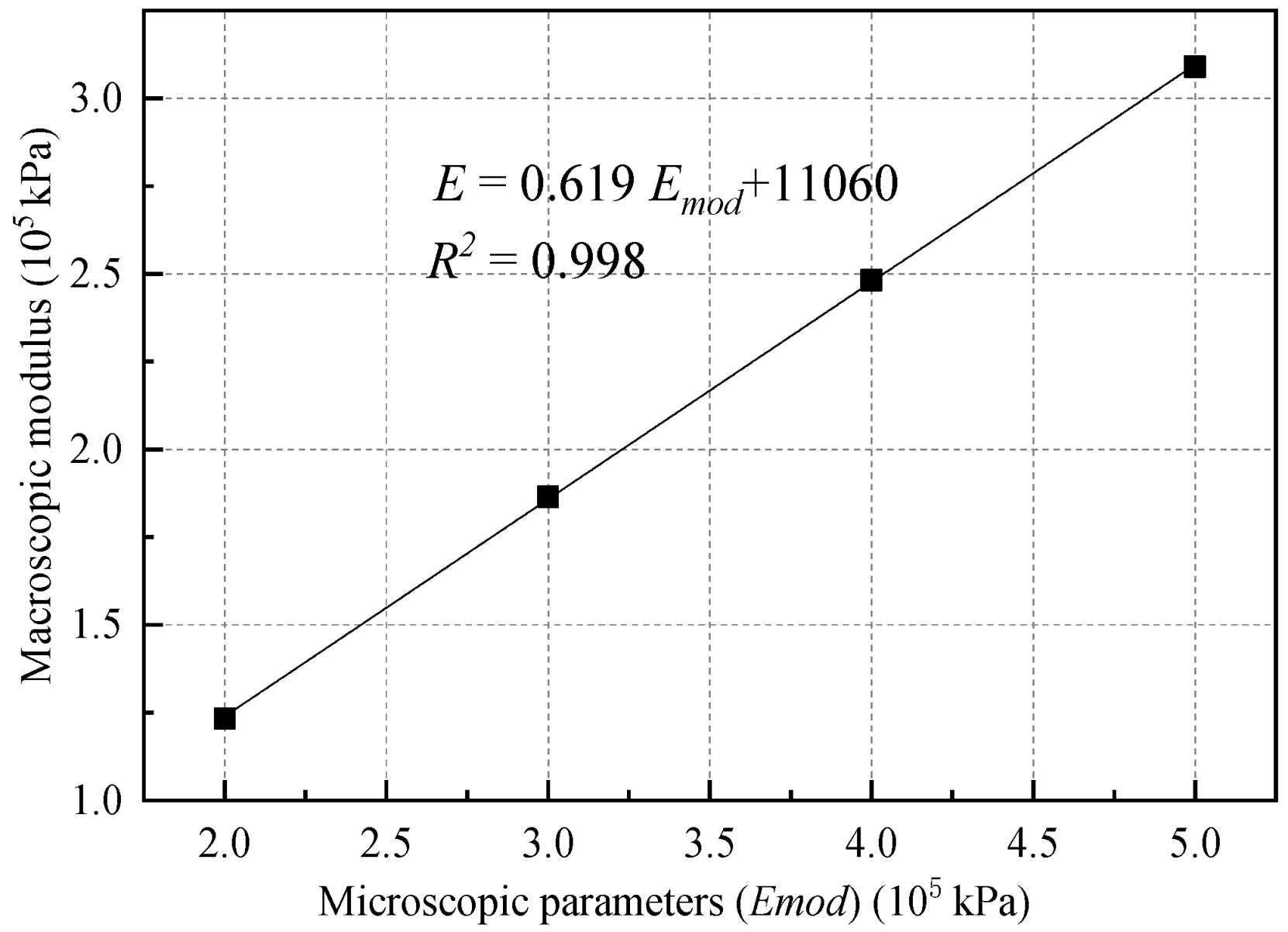
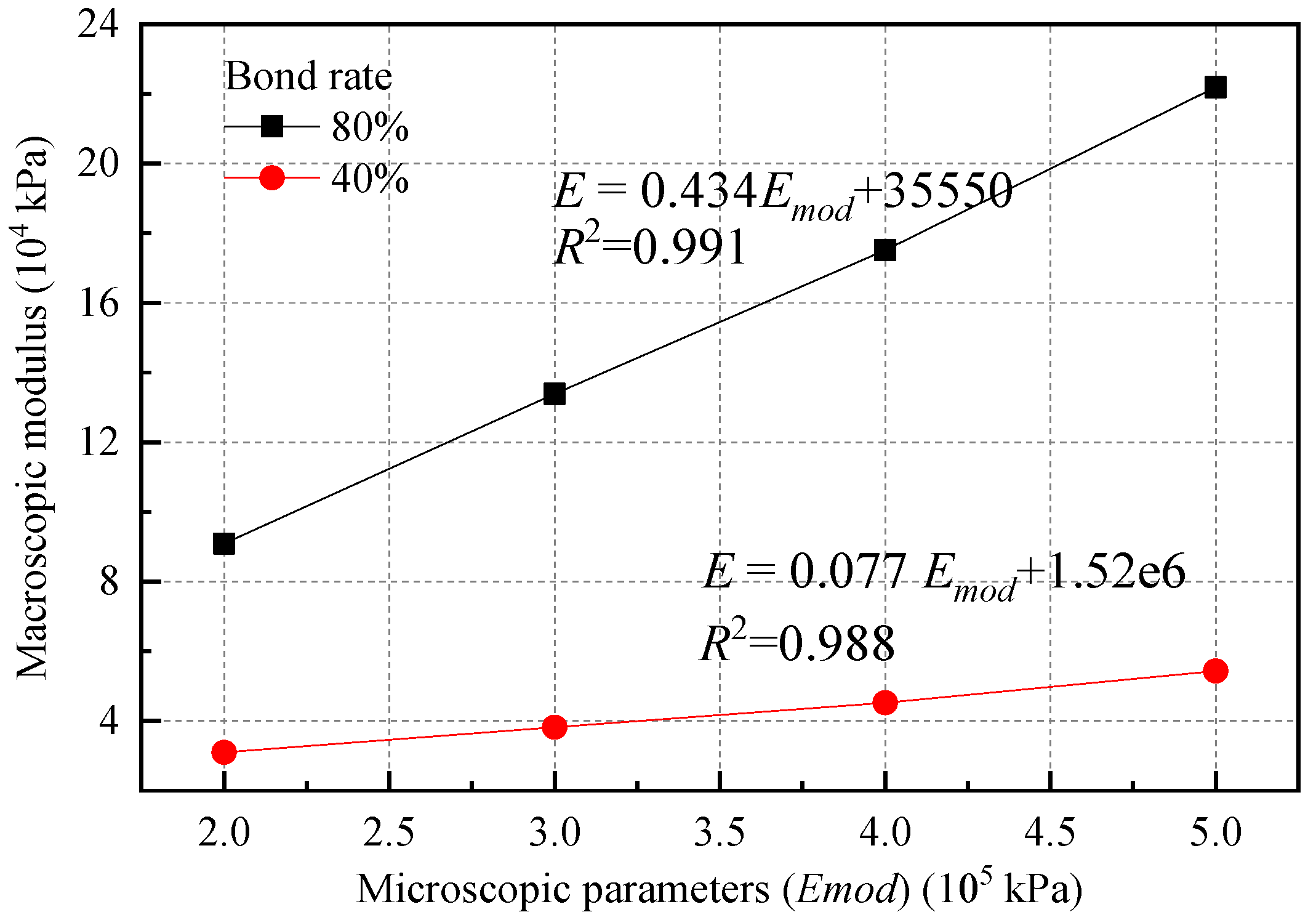
3.1.1. Equivalent Modulus
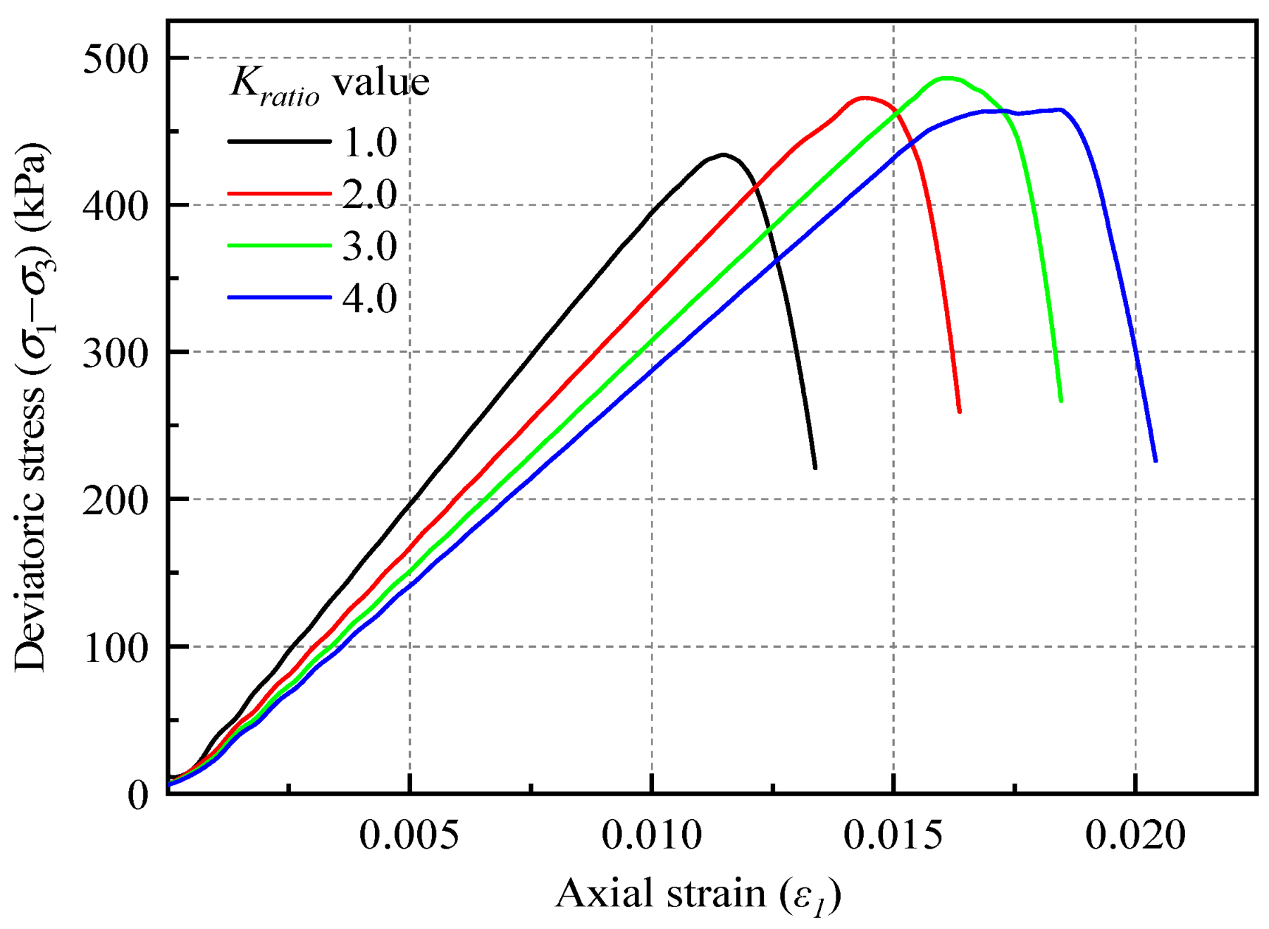
3.1.2. Normal and Tangential Stiffness Ratio
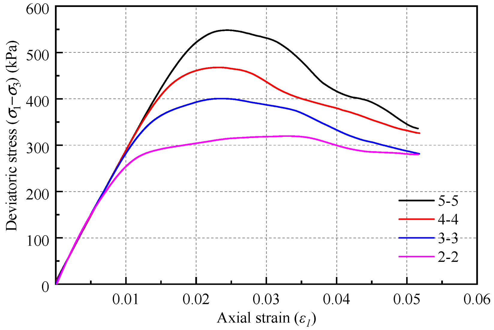
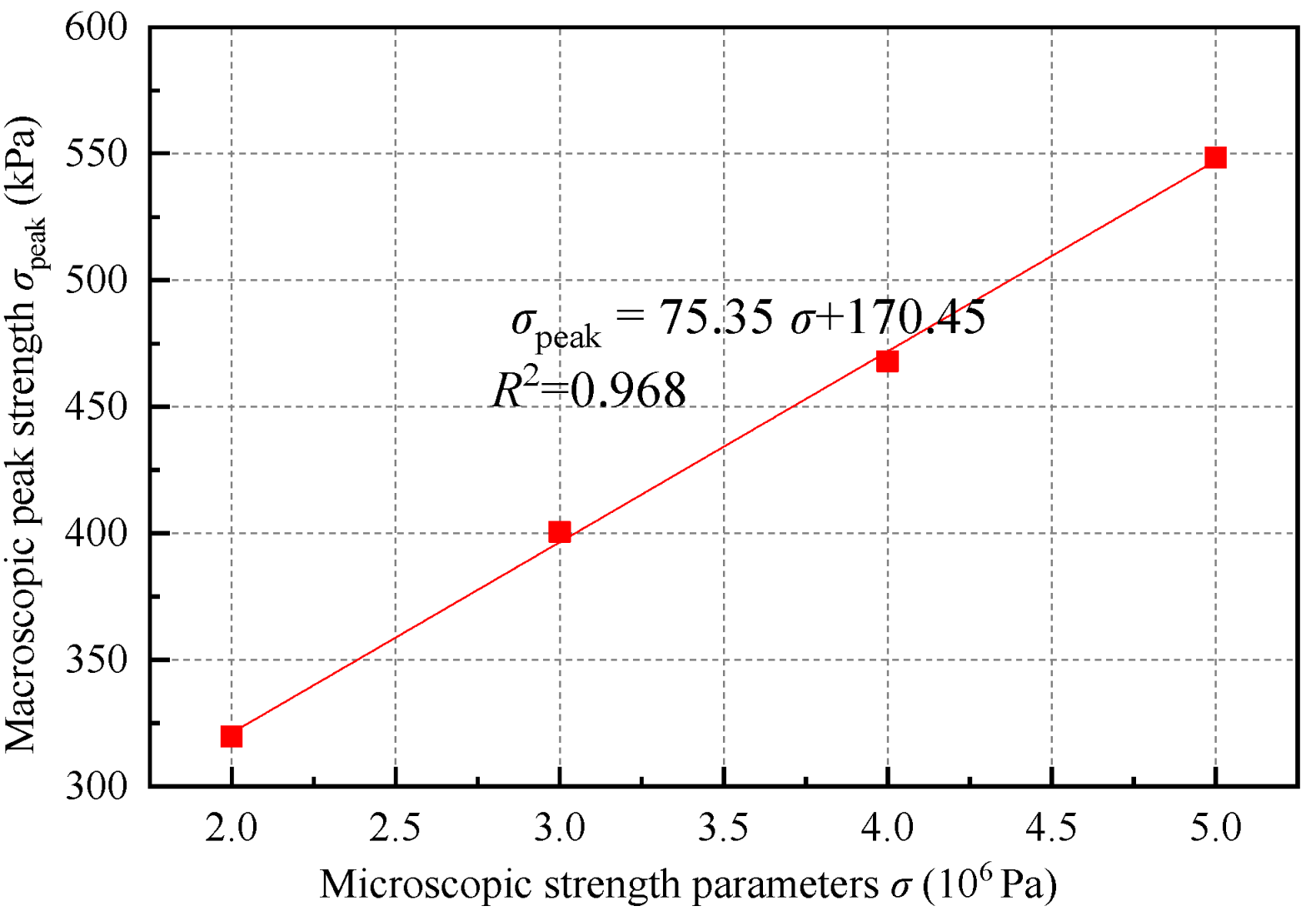
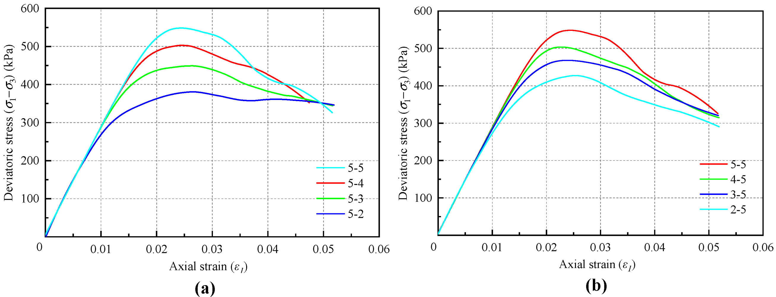
3.2. Contact Strength
3.2.1. Proportional Change
3.2.2. Relative Values
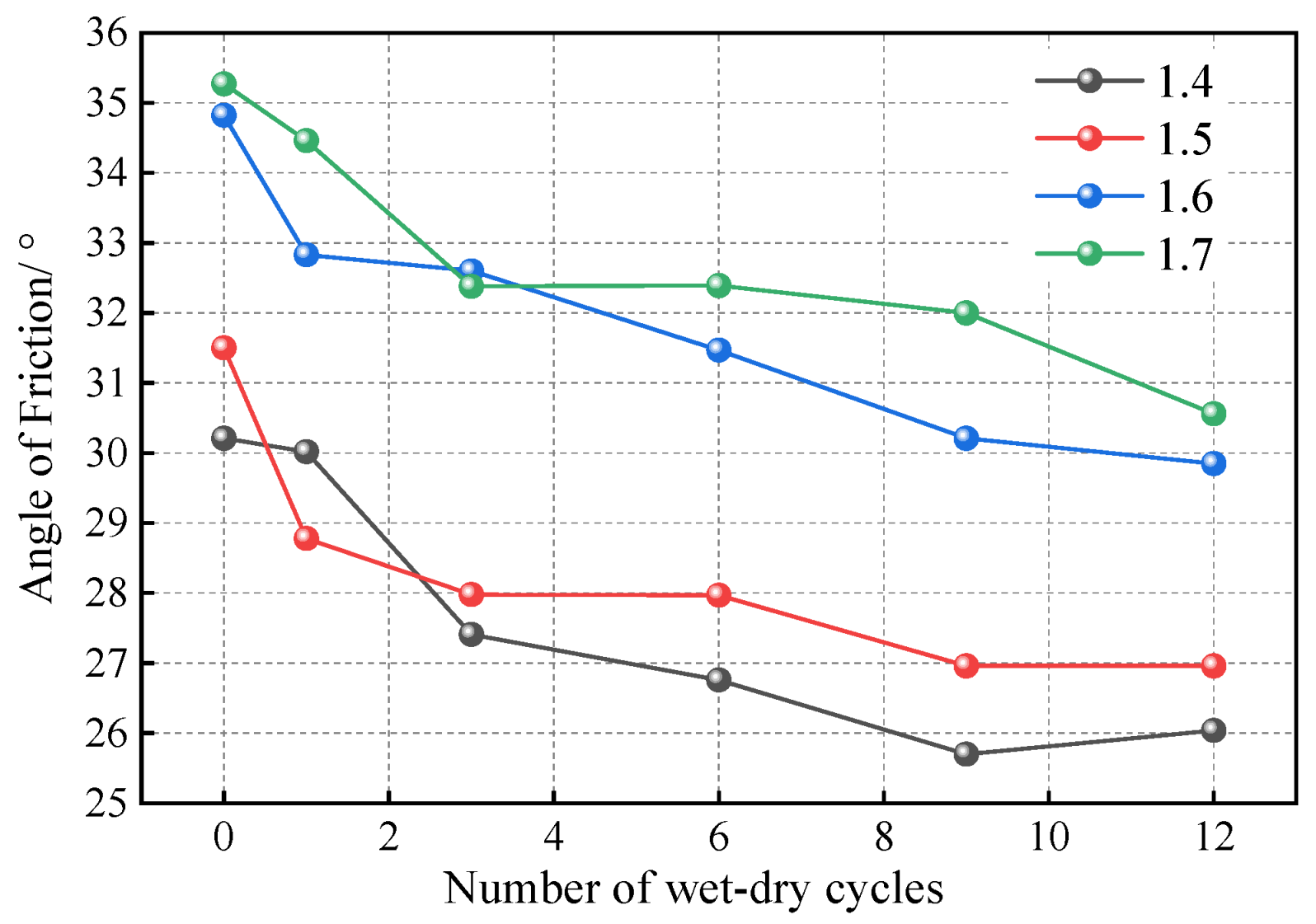
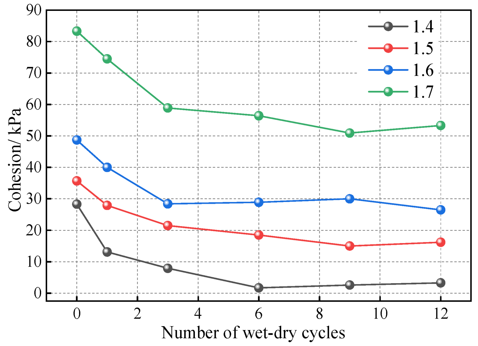
3.3. Friction Coefficient
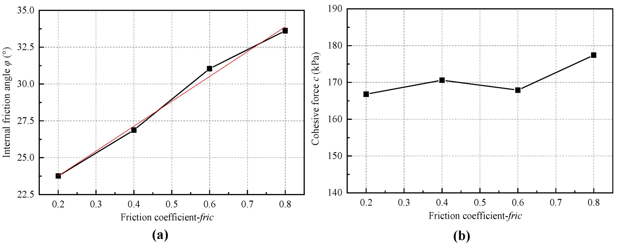
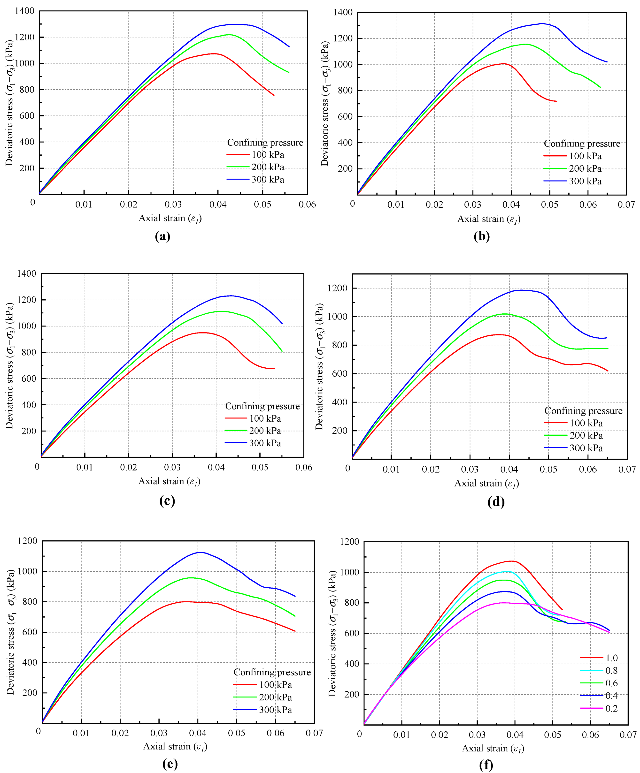
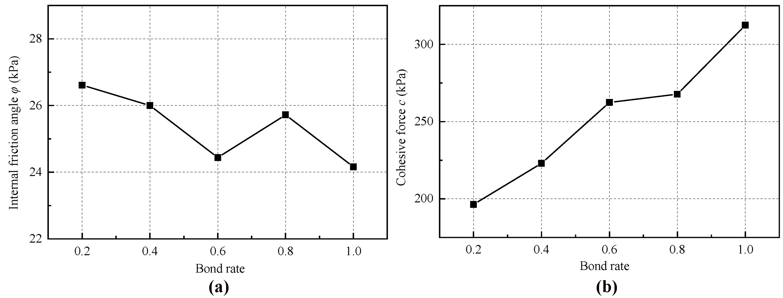
3.4. Bond Rate
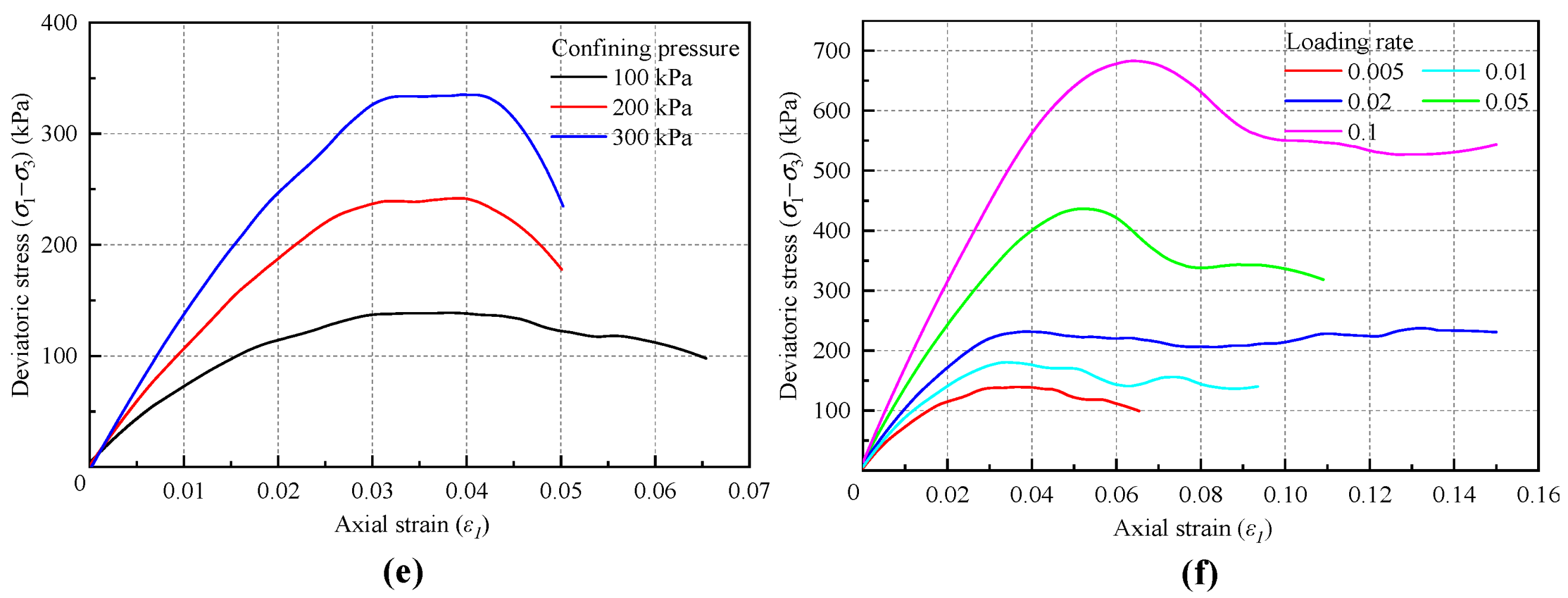
3.5. Loading Rate
3.6. Macro Significance of Microscopic Parameters
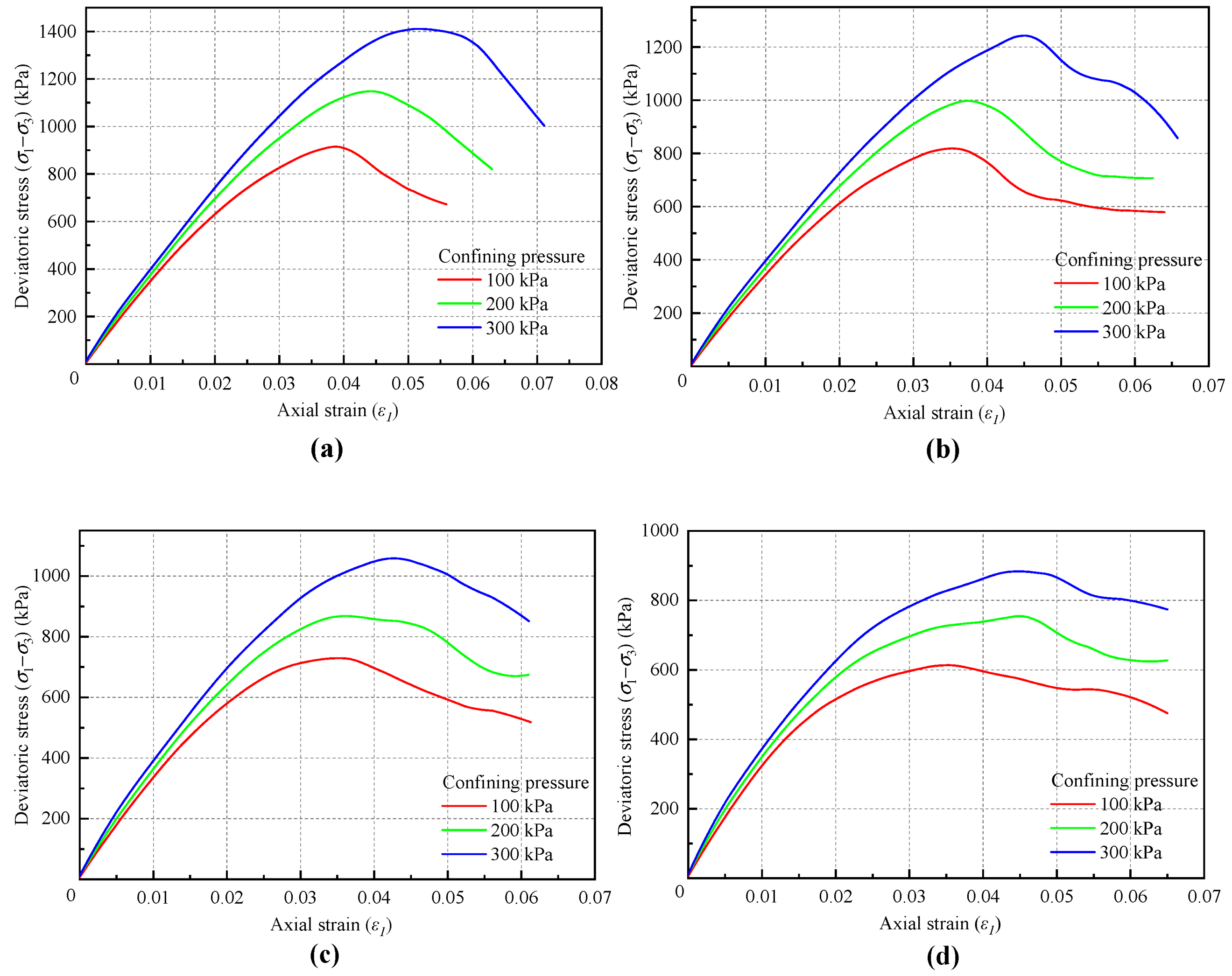
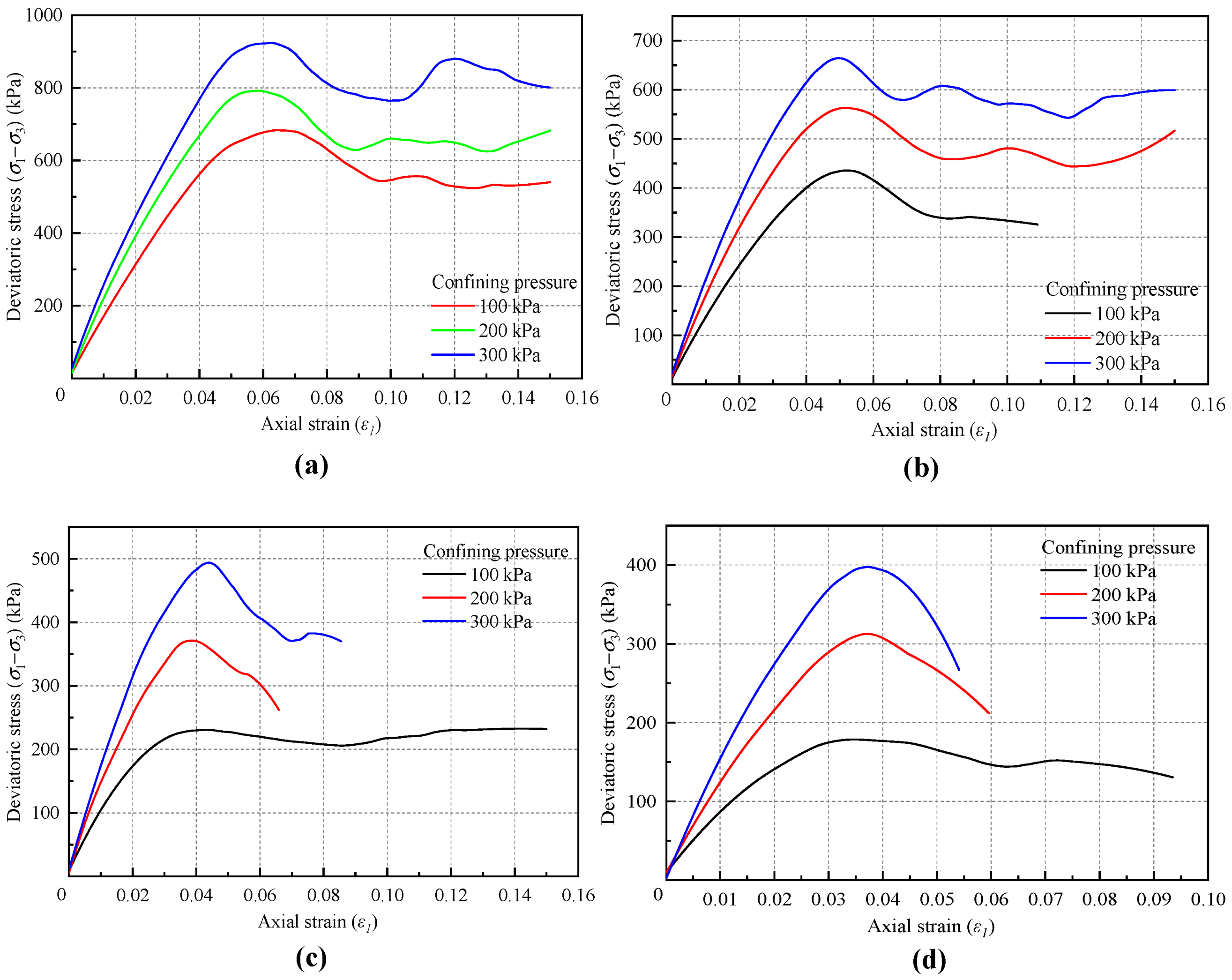
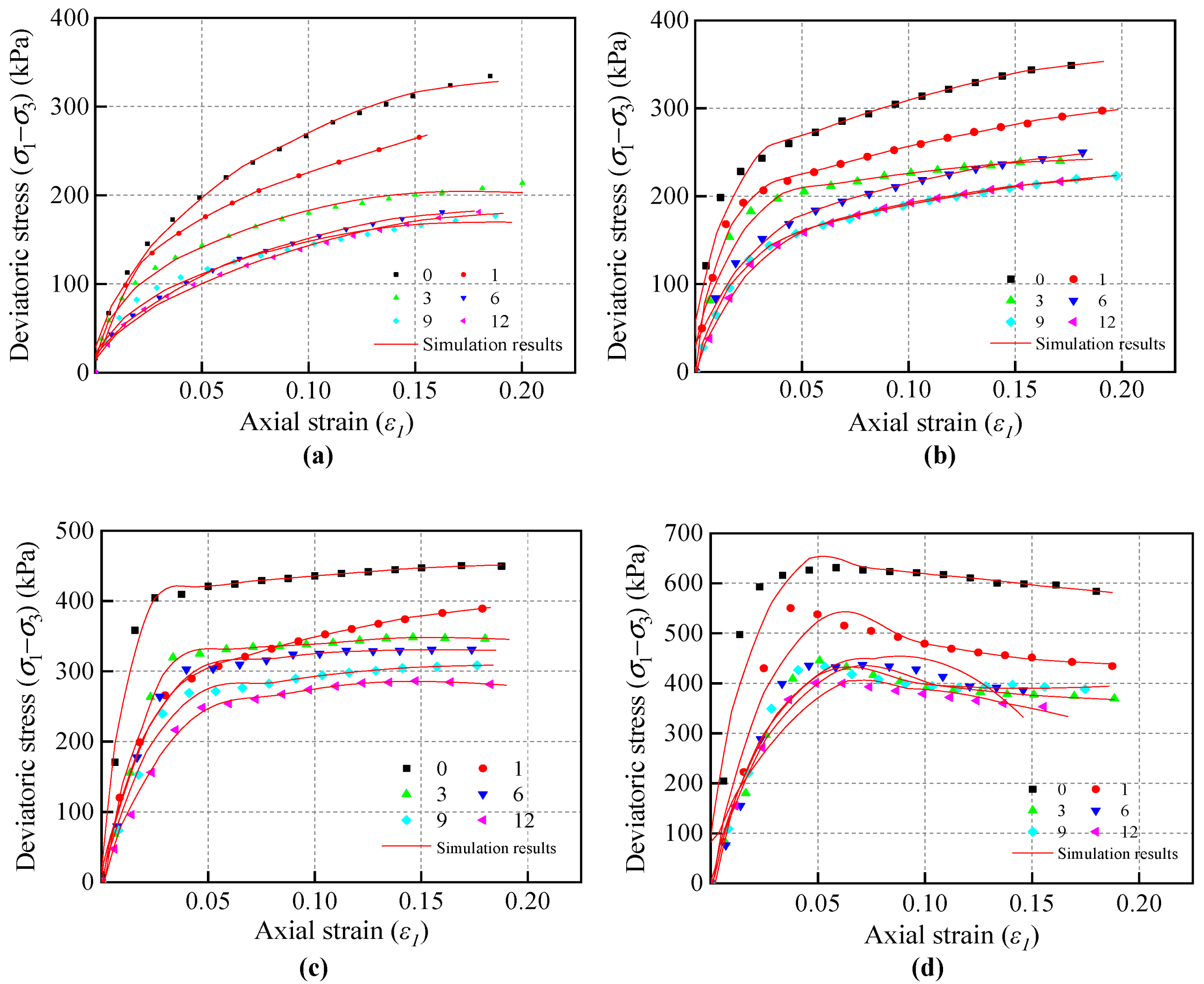
4. Model Applications
5. Discussion
6. Conclusions
Author Contributions
Funding
Institutional Review Board Statement
Informed Consent Statement
Data Availability Statement
Conflicts of Interest
References
- Wu, D.; Zhao, Z.; Gao, H. An Interface-Enhanced Discrete Element Model (I-DEM) of Bio-Inspired Flexible Protective Structures. Comput. Methods Appl. Mech. Eng. 2024, 420, 116702. [Google Scholar] [CrossRef]
- Hu, C.; Yuan, Y.; Mei, Y.; Wang, X.; Liu, Z. Comprehensive Strength Deterioration Model of Compacted Loess Exposed to Drying-Wetting Cycles. Bull. Eng. Geol. Environ. 2020, 79, 383–398. [Google Scholar] [CrossRef]
- Xu, J.; Zhou, L.; Hu, K.; Li, Y.; Zhou, X.; Wang, S. Influence of Wet-Dry Cycles on Uniaxial Compression Behavior of Fissured Loess Disturbed by Vibratory Loads. KSCE J. Civ. Eng. 2022, 26, 2139–2152. [Google Scholar] [CrossRef]
- Shi, Q.; Wang, B.; Mao, H.; Liu, Y. Calibration and Measurement of Micrometre-Scale Pollen Particles for Discrete Element Method Parameters Based on the Johnson-Kendal-Roberts Model. Biosyst. Eng. 2024, 237, 83–91. [Google Scholar] [CrossRef]
- Tang, Z.-Q.; Yin, Z.-Y.; Jin, Y.-F.; Zhou, X.-W. A Novel Mesoscale Modelling Method for Steel Fibre-Reinforced Concrete with the Combined Finite-Discrete Element Method. Cem. Concr. Compos. 2024, 149, 105479. [Google Scholar] [CrossRef]
- Wang, X.; Mei, Y.; Yuan, Y.; Wang, R.; Zhou, D. Research on the Soil-Plugging Effect on Small-Diameter Jacked Piles through In Situ Testing and DEM Simulation. Buildings 2022, 12, 2022. [Google Scholar] [CrossRef]
- Bouckaert, I.; Godio, M.; Pacheco De Almeida, J. A Hybrid Discrete-Finite Element Method for Continuous and Discontinuous Beam-like Members Including Nonlinear Geometric and Material Effects. Int. J. Solids Struct. 2024, 294, 112770. [Google Scholar] [CrossRef]
- Zhao, T.; Collins, P.E.F. Modelling the Brittle Rock Failure by the Quaternion-Based Bonded-Particle Model in DEM. Rock Mech. Bull. 2024, 3, 100115. [Google Scholar] [CrossRef]
- Ismail, Y.; Yang, D.; Ye, J. A DEM Model for Visualising Damage Evolution and Predicting Failure Envelope of Composite Laminae under Biaxial Loads. Compos. Part B Eng. 2016, 102, 9–28. [Google Scholar] [CrossRef]
- Huang, J.; Song, Y.; Lei, M.; Shi, C.; Jia, C.; Zhang, J. Numerical Study on the Damage Characteristics of Layered Shale Using 3D DEM. KSCE J. Civ. Eng. 2023, 27, 5436–5447. [Google Scholar] [CrossRef]
- Jin, X.; Li, X.; Huang, Y. DEM Analysis on Diffuse Failure of Soil Slope Triggered by Earthquakes. Eng. Geol. 2024, 339, 107640. [Google Scholar] [CrossRef]
- Jiang, M.; Jiang, T.; Crosta, G.B.; Shi, Z.; Chen, H.; Zhang, N. Modeling Failure of Jointed Rock Slope with Two Main Joint Sets Using a Novel DEM Bond Contact Model. Eng. Geol. 2015, 193, 79–96. [Google Scholar] [CrossRef]
- Hassan, S.; El Shamy, U. DEM Simulations of the Seismic Response of Granular Slopes. Comput. Geotech. 2019, 112, 230–244. [Google Scholar] [CrossRef]
- Rougier, E.; Munjiza, A.; Lei, Z.; Chau, V.T.; Knight, E.E.; Hunter, A.; Srinivasan, G. The Combined Plastic and Discrete Fracture Deformation Framework for Finite-discrete Element Methods. Numer. Methods Eng. 2020, 121, 1020–1035. [Google Scholar] [CrossRef]
- Meza-Lopez, J.; Noreña, N.; Meza, C.; Romanel, C. Modeling of Asphalt Concrete Fracture Tests with the Discrete-Element Method. J. Mater. Civ. Eng. 2020, 32, 04020228. [Google Scholar] [CrossRef]
- Zhang, W.; Rothenburg, L. Comparison of Undrained Behaviors of Granular Media Using Fluid-Coupled Discrete Element Method and Constant Volume Method. J. Rock Mech. Geotech. Eng. 2020, 12, 1272–1289. [Google Scholar] [CrossRef]
- Chen, D.; Sun, C.; Wang, L. Collapse Behavior and Control of Hard Roofs in Steeply Inclined Coal Seams. Bull. Eng. Geol. Environ. 2021, 80, 1489–1505. [Google Scholar] [CrossRef]
- Shi, L.; Zhao, W.; Sun, B.; Sun, W. Determination of the Coefficient of Rolling Friction of Irregularly Shaped Maize Particles by Using Discrete Element Method. Int. J. Agric. Biol. Eng. 2020, 13, 15–25. [Google Scholar] [CrossRef]
- Nie, Z.; Liu, S.; Hu, W.; Gong, J. Effect of Local Non-Convexity on the Critical Shear Strength of Granular Materials Determined via the Discrete Element Method. Particuology 2020, 52, 105–112. [Google Scholar] [CrossRef]
- Liu, X.; Gui, N.; Yang, X.; Tu, J.; Jiang, S. A New Discrete Element-Embedded Finite Element Method for Transient Deformation, Movement and Heat Transfer in Packed Bed. Int. J. Heat Mass Transf. 2021, 165, 120714. [Google Scholar] [CrossRef]
- Kuang, D.-M.; Long, Z.-L.; Ogwu, I.; Chen, Z. A Discrete Element Method (DEM)-Based Approach to Simulating Particle Breakage. Acta Geotech. 2022, 17, 2751–2764. [Google Scholar] [CrossRef]
- De, T.; Chakraborty, J.; Kumar, J.; Tripathi, A.; Sen, M.; Ketterhagen, W. A Particle Location Based Multi-Level Coarse-Graining Technique for Discrete Element Method (DEM) Simulation. Powder Technol. 2022, 398, 117058. [Google Scholar] [CrossRef]
- Liu, G.; Han, D.; Jia, Y.; Zhao, Y. Asphalt Mixture Skeleton Main Force Chains Composition Criteria and Characteristics Evaluation Based on Discrete Element Methods. Constr. Build. Mater. 2022, 323, 126313. [Google Scholar] [CrossRef]
- Li, Z.; Chow, J.K.; Li, J.; Tai, P.; Zhou, Z. Modeling of Flexible Membrane Boundary Using Discrete Element Method for Drained/Undrained Triaxial Test. Comput. Geotech. 2022, 145, 104687. [Google Scholar] [CrossRef]
- Tang, W.; Zhai, C.; Xu, J.; Yu, X.; Sun, Y.; Cong, Y.; Zheng, Y.; Zhu, X. Numerical Simulation of Expansion Process of Soundless Cracking Demolition Agents by Coupling Finite Difference and Discrete Element Methods. Comput. Geotech. 2022, 146, 104699. [Google Scholar] [CrossRef]
- Qu, Y.; Zou, D.; Liu, J.; Yang, Z.; Chen, K. Two-Dimensional DEM-FEM Coupling Analysis of Seismic Failure and Anti-Seismic Measures for Concrete Faced Rockfill Dam. Comput. Geotech. 2022, 151, 104950. [Google Scholar] [CrossRef]
- Hu, Z.; Yang, Z.X.; Guo, N.; Zhang, Y.D. Multiscale Modeling of Seepage-Induced Suffusion and Slope Failure Using a Coupled FEM–DEM Approach. Comput. Methods Appl. Mech. Eng. 2022, 398, 115177. [Google Scholar] [CrossRef]
- Zhang, S.; Li, B.; Ma, H. Numerical Investigation of Scour around the Monopile Using CFD-DEM Coupling Method. Coast. Eng. 2023, 183, 104334. [Google Scholar] [CrossRef]
- Li, J.; Wang, B.; Pan, P.; Chen, H.; Wang, D.; Chen, P. Failure Analysis of Soil-Rock Mixture Slopes Using Coupled MPM-DEM Method. Comput. Geotech. 2024, 169, 106226. [Google Scholar] [CrossRef]
- Ahmadian, M.H.; Zheng, W. Simulating the Fluid–Solid Interaction of Irregularly Shaped Particles Using the LBM-DEM Coupling Method. Comput. Geotech. 2024, 171, 106395. [Google Scholar] [CrossRef]
- Chen, J.; Wang, L.; Yang, S.; Zhang, J. Semi-Resolved CFD–DEM Coupling Simulation of Wave Interaction with Submerged Permeable Breakwaters. Ocean Eng. 2025, 321, 120411. [Google Scholar] [CrossRef]
- Yu, M.; Yang, B.; Chi, Y.; Xie, J.; Ye, J. Experimental Study and DEM Modelling of Bolted Composite Lap Joints Subjected to Tension. Compos. Part B Eng. 2020, 190, 107951. [Google Scholar] [CrossRef]
- Wang, S.; Hu, J.; Ji, J.; Zhou, H.; Pang, J. Experimental Study and Computer Simulation of Compression Characteristics and Crushing of Chinese Cabbage Seeds. Appl. Eng. Agric. 2020, 36, 815–825. [Google Scholar] [CrossRef]
- Zhao, M.; Liu, H.; Ma, Q.; Xing, L.; Xia, Q.; Yang, X.; Li, F.; Li, X. Discrete Element Simulation Analysis of Damage and Failure of Hydrate-Bearing Sediments. J. Nat. Gas Sci. Eng. 2022, 102, 104557. [Google Scholar] [CrossRef]
- Novak, J.K.; Selvarathinam, A.S. A Comparison of Discrete Damage Modeling Methods: The Effect of Stacking Sequence on Progressive Failure of the Skin Laminate in a Composite Pi-Joint Subject to Pull-off Load. In Proceedings of the AIAA Scitech 2021 Forum, American Institute of Aeronautics and Astronautics, Virtual Event, 11–15 January 2021. [Google Scholar]
- Kosteski, L.E.; Iturrioz, I.; Friedrich, L.F.; Lacidogna, G. A Study by the Lattice Discrete Element Method for Exploring the Fractal Nature of Scale Effects. Sci. Rep. 2022, 12, 16744. [Google Scholar] [CrossRef]
- Dong, X.; Zheng, H.; Jia, X.; Li, Y.; Song, J.; Wang, J. Calibration and experiments of the discrete element simulation parameters for rice bud damage. INMATEH Agric. Eng. 2022, 68, 659–668. [Google Scholar] [CrossRef]
- Liu, W.; Su, Q.; Fang, M.; Zhang, J.; Zhang, W.; Yu, Z. Parameters Calibration of Discrete Element Model for Corn Straw Cutting Based on Hertz-Mindlin with Bonding. Appl. Sci. 2023, 13, 1156. [Google Scholar] [CrossRef]
- Peng, Y.; Chen, Y.; Xu, Y.; Xia, S.; Lu, X.; Li, Y. Discrete Element Modelling of Mechanical Response of Crumb Rubber-Modified Asphalt Pavements under Traffic Loads. Int. J. Pavement Eng. 2023, 24, 2068546. [Google Scholar] [CrossRef]
- Zhu, Y.; Yan, Y.; Zhang, Y.; Zhang, W.; Kong, J.; Dai, A. Study on the Evolution Law of Overlying Strata Structure in Stope Based on “Space–Air–Ground” Integrated Monitoring Network and Discrete Element. Drones 2023, 7, 309. [Google Scholar] [CrossRef]
- Xue, B.; Que, Y.; Pei, J.; Ma, X.; Wang, D.; Yuan, Y.; Zhang, H. A State-of-the-Art Review of Discrete Element Method for Asphalt Mixtures: Model Generation Methods, Contact Constitutive Models and Application Directions. Constr. Build. Mater. 2024, 414, 134842. [Google Scholar] [CrossRef]
- Gong, F.; Deng, R.; Wang, Q.; Bai, J.; Cheng, X. A Review on the Simulation of Aggregate Morphologies in Mixture Performances Based on Discrete Element Method. Constr. Build. Mater. 2023, 385, 131522. [Google Scholar] [CrossRef]
- Ding, H.; Han, Z.; Li, Y.; Xie, W.; Fu, B.; Li, C.; Zhao, L. Particle Breakage and Its Mechanical Response in Granular Soils: A Review and Prospect. Constr. Build. Mater. 2023, 409, 133948. [Google Scholar] [CrossRef]
- Potyondy, D.O.; Cundall, P.A. A Bonded-Particle Model for Rock. Int. J. Rock Mech. Min. Sci. 2004, 41, 1329–1364. [Google Scholar] [CrossRef]
- Li, Y.; Xu, L.; Ma, Z.; Ma, B.; Zhang, J. Numerical Simulation of the Critical Hydraulic Gradient of Granular Soils at Seepage Failure by Discrete Element Method and Computational Fluid Dynamics. J. Hydro-Environ. Res. 2024, 53, 1–14. [Google Scholar] [CrossRef]
- Cho, N.; Martin, C.D.; Sego, D.C. A Clumped Particle Model for Rock. Int. J. Rock Mech. Min. Sci. 2007, 44, 997–1010. [Google Scholar] [CrossRef]


| Dry Density (g/cm3) | 3D Void Ratio e3d | 3D Porosity n3d | 2D Porosity n2d | Particle Number |
|---|---|---|---|---|
| 1.4 | 0.94 | 0.49 | 0.23 | 6397 |
| 1.5 | 0.81 | 0.45 | 0.22 | 6547 |
| 1.6 | 0.70 | 0.41 | 0.20 | 6710 |
| 1.7 | 0.60 | 0.38 | 0.19 | 6880 |
| Microscopic Emod (105 kPa) | 2 | 3 | 4 | 5 |
| Macroscopic modulus (105 kPa) | 1.23 | 1.86 | 2.48 | 3.09 |
| Microscopic Emod (105 kPa) | 2 | 3 | 4 | 5 |
|---|---|---|---|---|
| Macroscopic modulus (80%) (105 kPa) | 0.9096 | 1.339 | 1.751 | 2.219 |
| Macroscopic modulus (40%) (105 kPa) | 0.310 | 0.383 | 0.453 | 0.543 |
| Microscopic Emod (105 kPa) | 1.0 | 2.0 | 3.0 | 4.0 |
| Macroscopic modulus (80%) (105 kPa) | 3.982 | 3.419 | 3.107 | 2.903 |
| Strength combination | 5-5 | 4-4 | 3-3 | 2-2 |
| Macroscopic peak strength (kPa) | 548.4 | 468.0 | 400.6 | 319.7 |
| Bond rate | 0.2 | 0.4 | 0.6 | 0.8 |
| Cohesive force (kPa) | 166.8 | 170.6 | 167.9 | 177.4 |
| Internal friction angle (°) | 23.76 | 26.88 | 31.04 | 33.62 |
| Bond rate | 0.2 | 0.4 | 0.6 | 0.8 | 1.0 |
| Cohesive force (kPa) | 196.4 | 223.0 | 262.4 | 267.7 | 312.4 |
| Internal friction angle (°) | 26.61 | 26 | 24.44 | 25.72 | 24.16 |
| Microscopic Parameters | Emod (105 kPa) | Kratio | cb_tens (103 kPa) | cb_shears (103 kPa) | fric |
|---|---|---|---|---|---|
| Value | 5 | 3.0 | 2 | 2 | 0.6 |
| Loading Rate (m/s) | Cohesive Force (kPa) | Internal Friction Angle (°) | The Fit Correlation Coefficient R2 | PFC Calculation Time (min) |
|---|---|---|---|---|
| 0.1 | 187.9 | 22.1 | 0.9996 | 11 |
| 0.05 | 111.1 | 21.35 | 0.9991 | 19 |
| 0.02 | 33.7 | 23.36 | 0.9997 | 29 |
| 0.01 | 26.2 | 20.79 | 0.9996 | 59 |
| 0.005 | 11.5 | 19.29 | 0.9992 | 128 |
| Number of Wet–Dry Cycles | Dry Density (g/cm3) | |||
|---|---|---|---|---|
| 1.4 | 1.5 | 1.6 | 1.7 | |
| 0 | 100% | 100% | 100% | 100% |
| 1 | 74.42% | 79.29% | 99.41% | 95.57% |
| 3 | 57.90% | 78.54% | 76.66% | 89.36% |
| 6 | 43.68% | 77.05% | 77.93% | 85.73% |
| 9 | 46.16% | 73.77% | 85.73% | 79.38% |
| 12 | 47.90% | 66.36% | 71.10% | 70.50% |
Disclaimer/Publisher’s Note: The statements, opinions and data contained in all publications are solely those of the individual author(s) and contributor(s) and not of MDPI and/or the editor(s). MDPI and/or the editor(s) disclaim responsibility for any injury to people or property resulting from any ideas, methods, instructions or products referred to in the content. |
© 2025 by the authors. Licensee MDPI, Basel, Switzerland. This article is an open access article distributed under the terms and conditions of the Creative Commons Attribution (CC BY) license (https://creativecommons.org/licenses/by/4.0/).
Share and Cite
Qi, H.; Liu, X.; Wang, H.; Hu, C. Discrete Element Damage Constitutive Model of Loess and Corresponding Parameter Sensitivity Analysis Based on the Bond Rate. Materials 2025, 18, 1726. https://doi.org/10.3390/ma18081726
Qi H, Liu X, Wang H, Hu C. Discrete Element Damage Constitutive Model of Loess and Corresponding Parameter Sensitivity Analysis Based on the Bond Rate. Materials. 2025; 18(8):1726. https://doi.org/10.3390/ma18081726
Chicago/Turabian StyleQi, Hui, Xiaoyan Liu, Haining Wang, and Chao Hu. 2025. "Discrete Element Damage Constitutive Model of Loess and Corresponding Parameter Sensitivity Analysis Based on the Bond Rate" Materials 18, no. 8: 1726. https://doi.org/10.3390/ma18081726
APA StyleQi, H., Liu, X., Wang, H., & Hu, C. (2025). Discrete Element Damage Constitutive Model of Loess and Corresponding Parameter Sensitivity Analysis Based on the Bond Rate. Materials, 18(8), 1726. https://doi.org/10.3390/ma18081726