
Through-Scale Numerical Investigation of Microstructure Evolution During the Cooling of Large-Diameter Rings


Highlights
- A pathway to more precise control of mechanical properties is achieved through process optimization.
- A hybrid FE thermal simulation combined with a CA microstructure evolution model.
- Complex macro- and micro-scale investigation of large-diameter steel ring cooling.
Abstract

1. Introduction
2. Materials and Methods
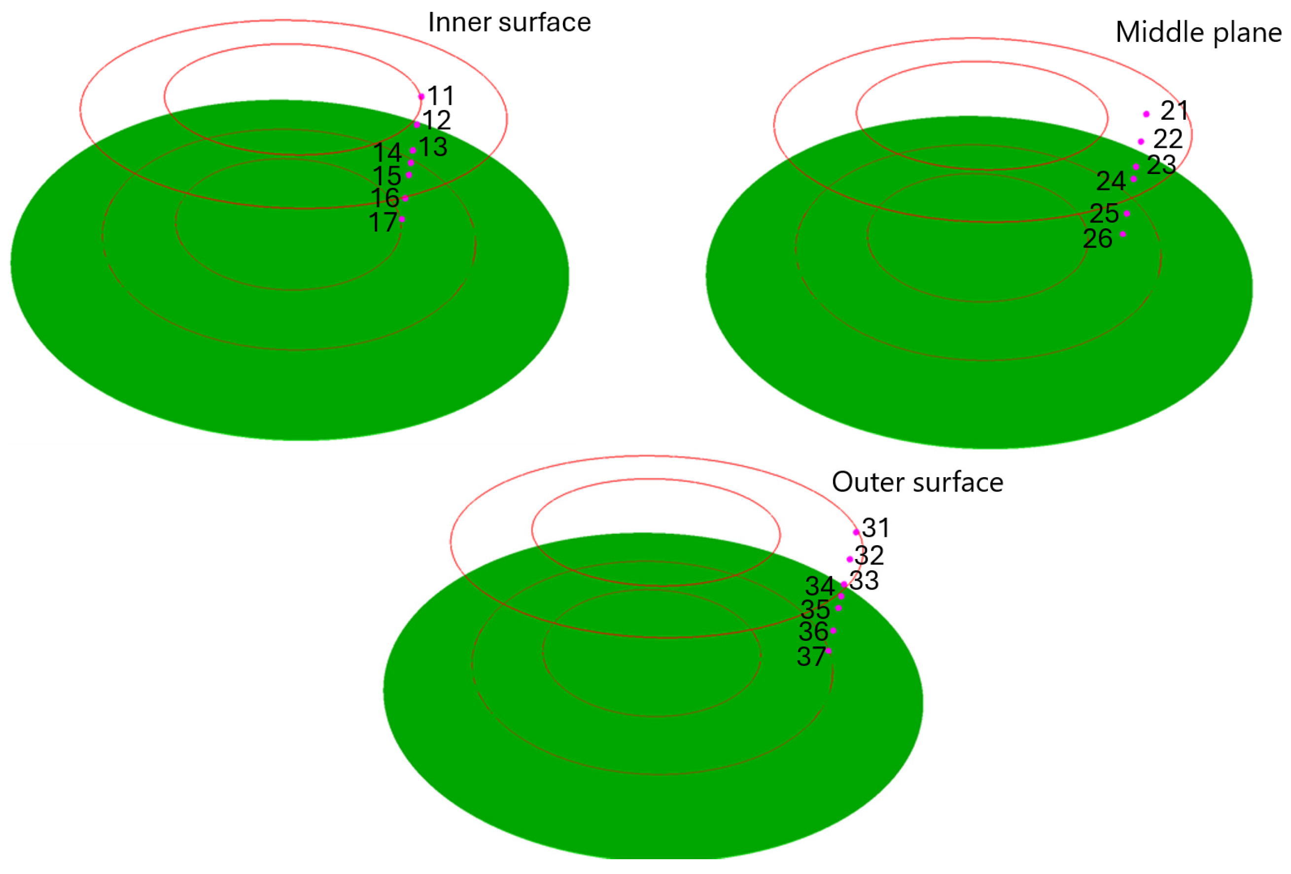
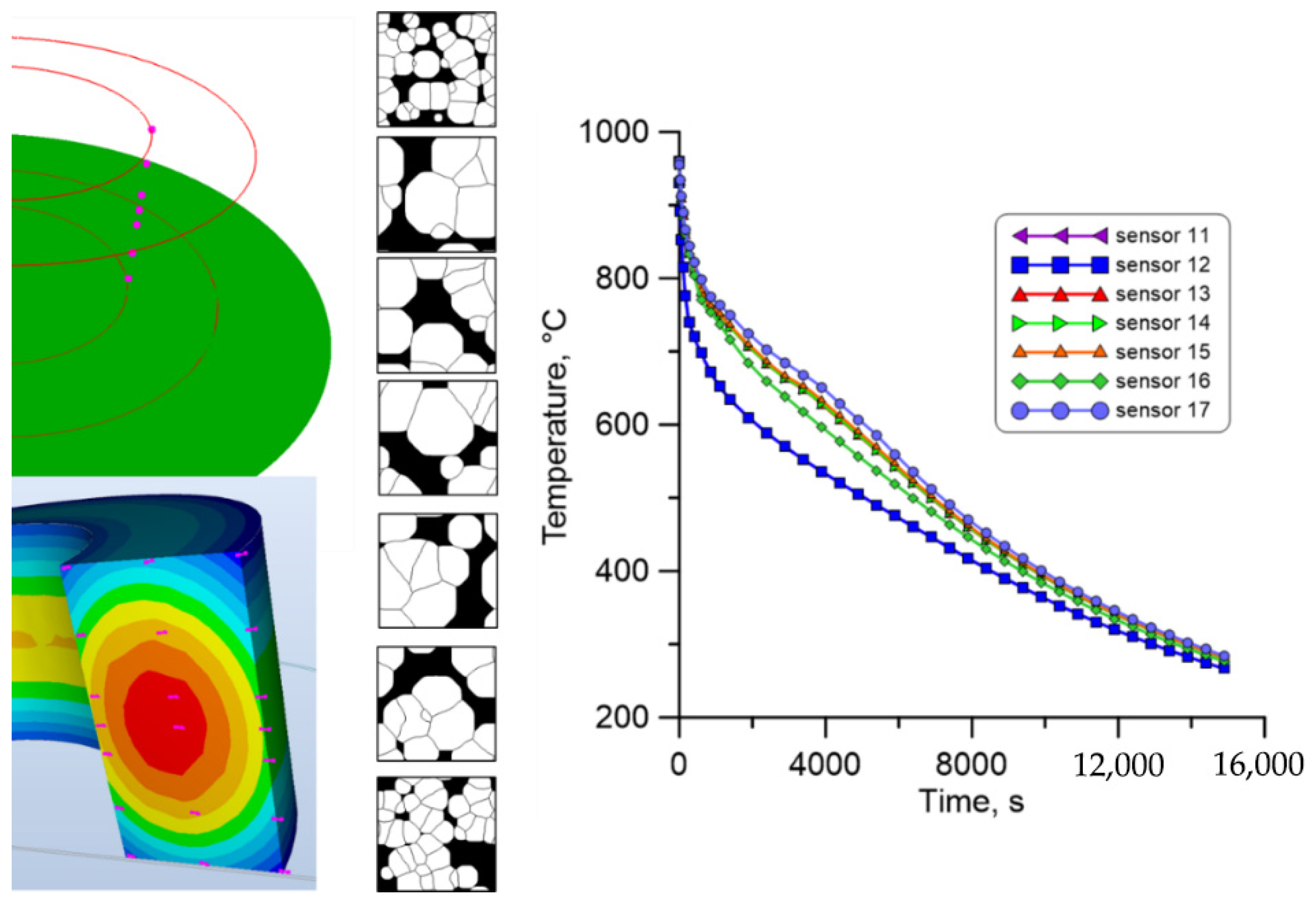
2.1. Cooling of Large-Diameter Rings
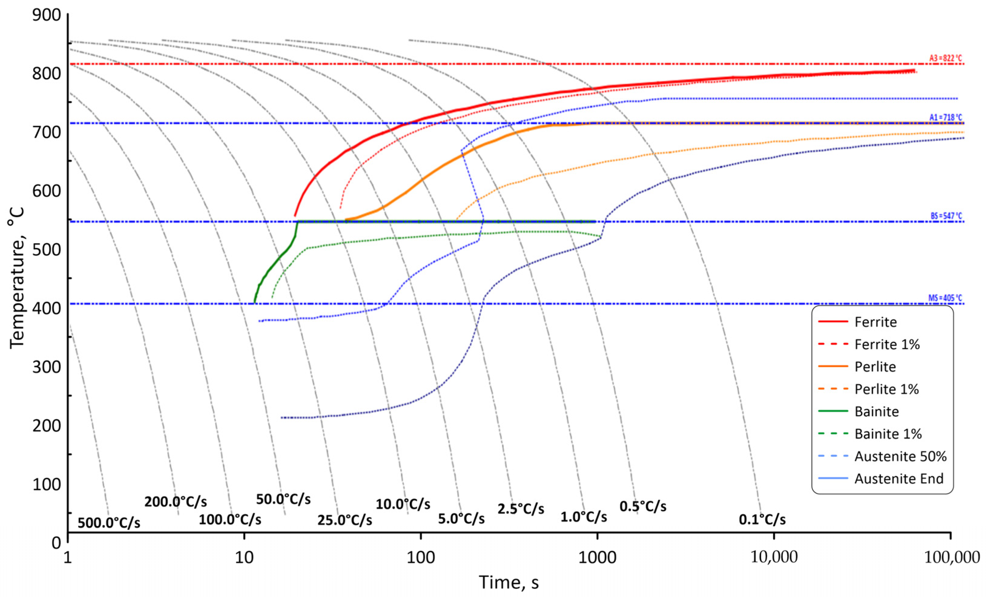
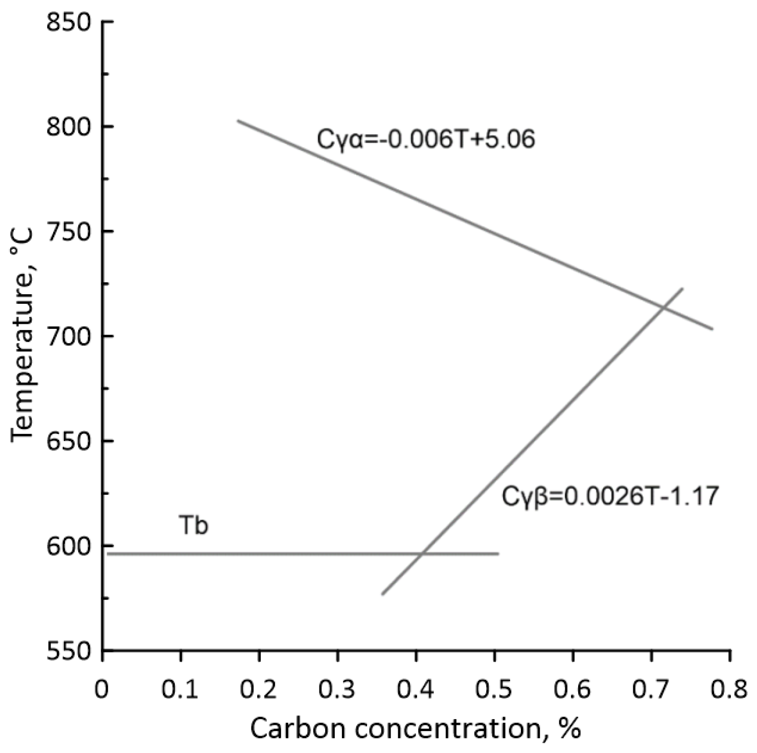
2.2. Cellular Automata Phase Transformation Model
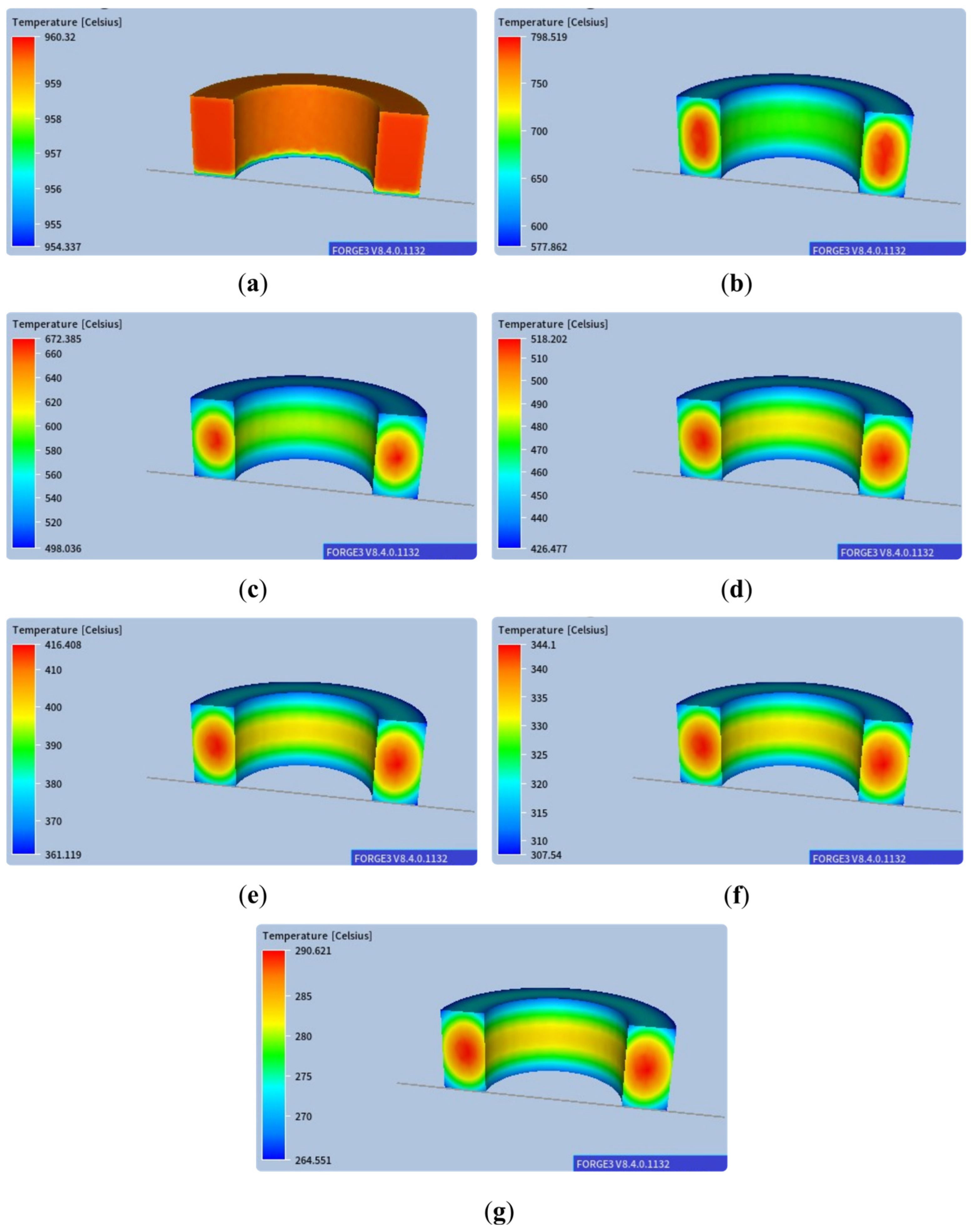
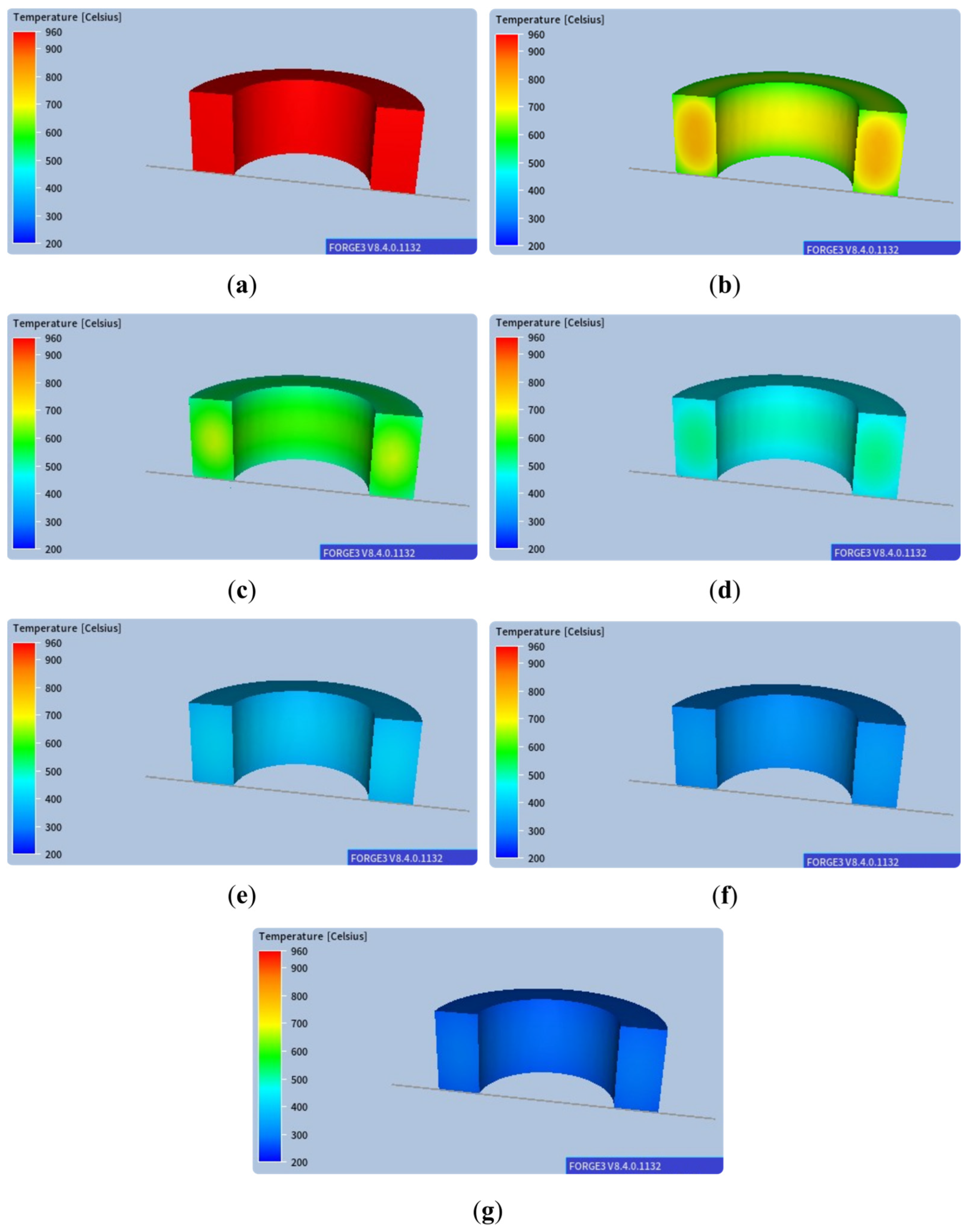
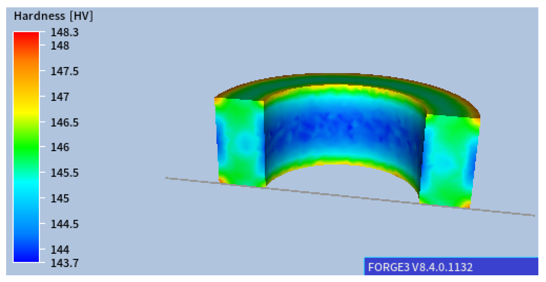
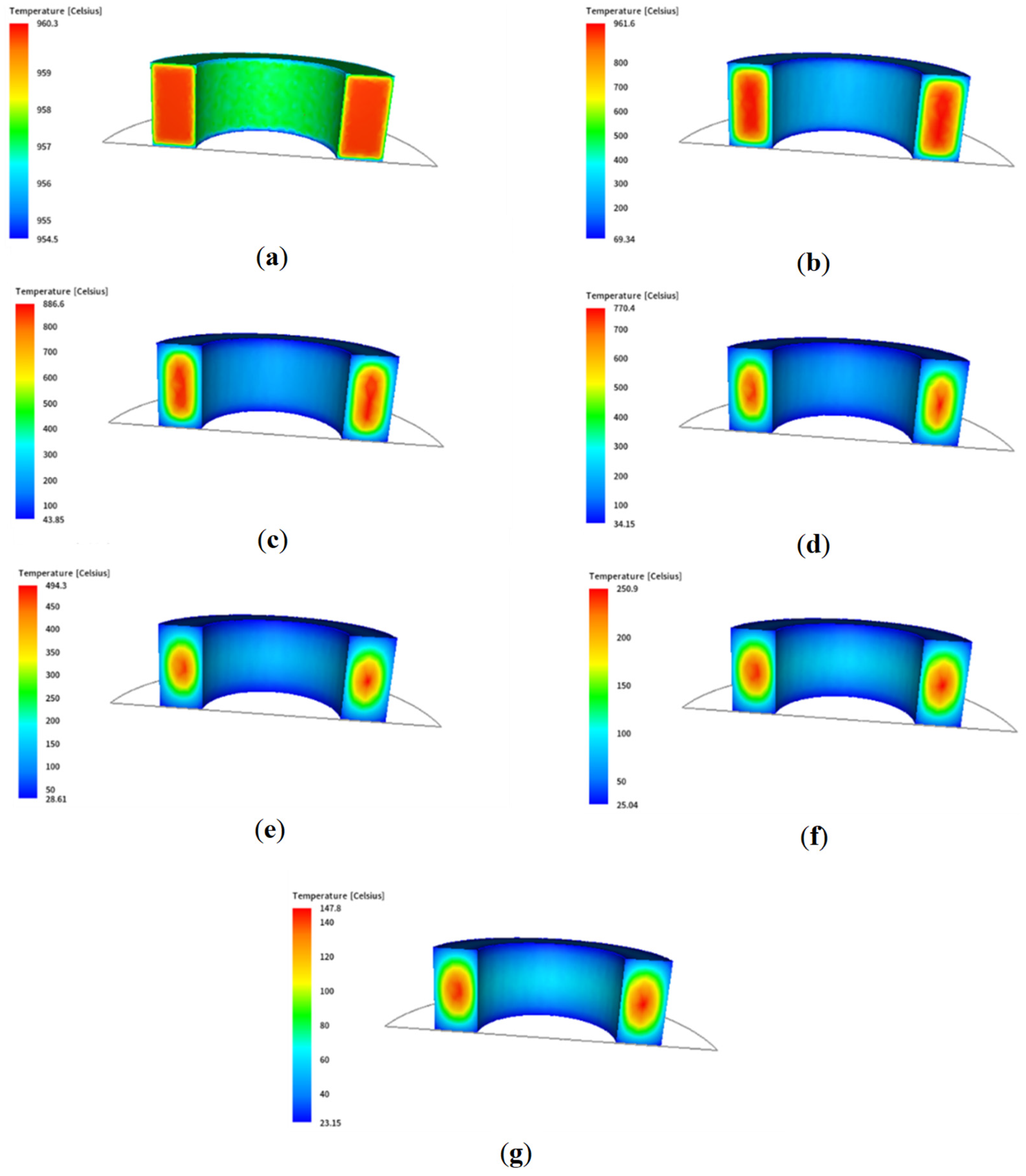
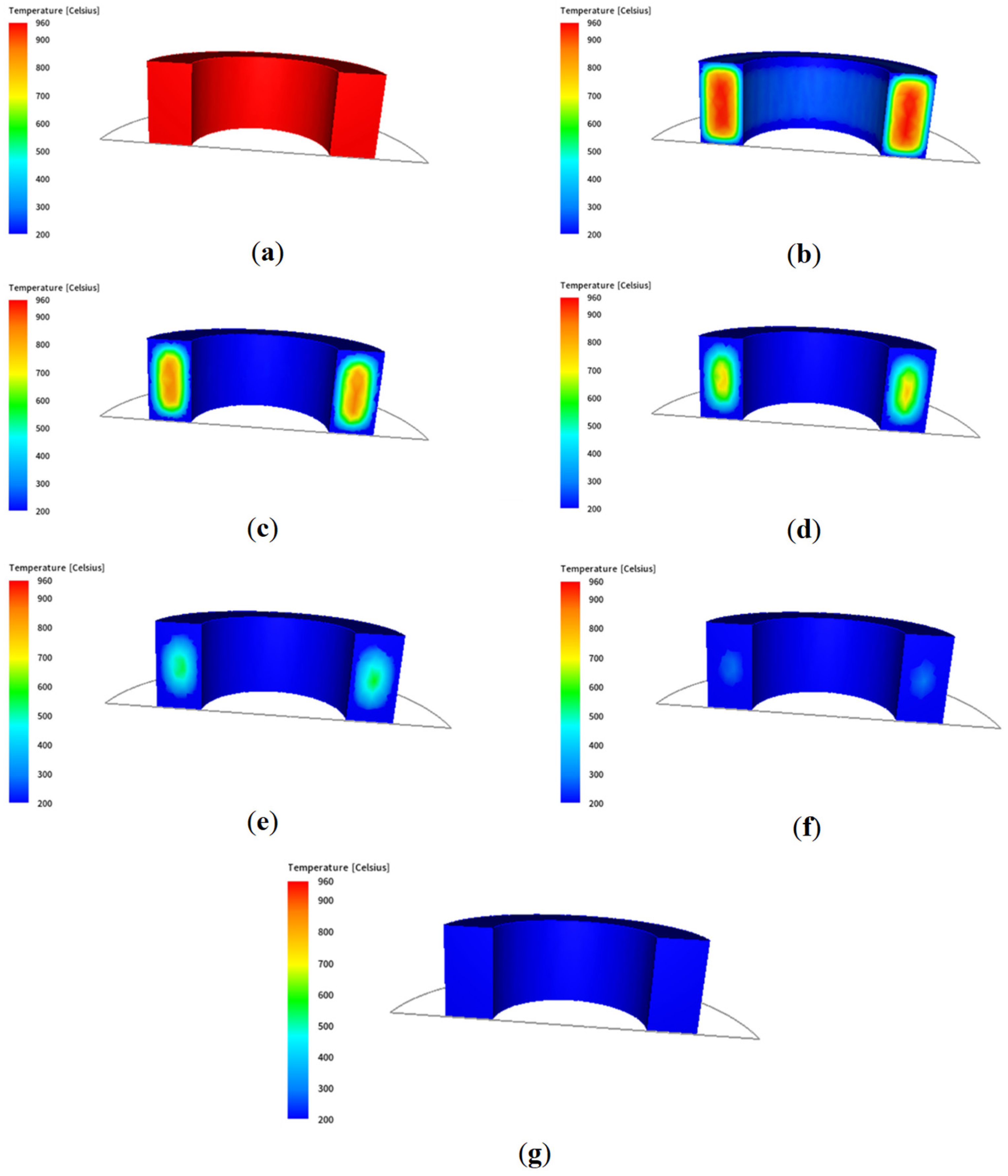
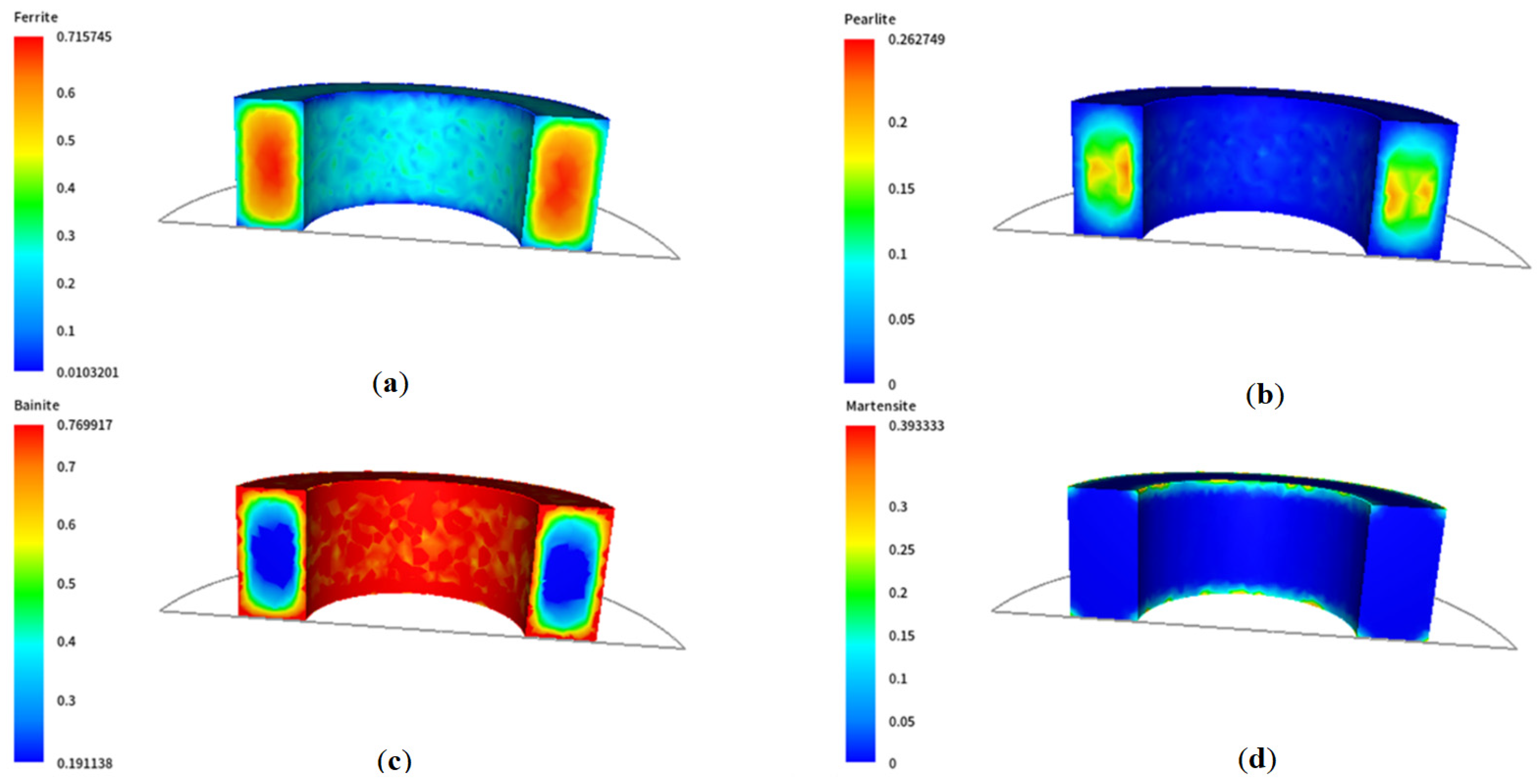
3. Results from Multiscale Modelling of the Large-Diameter Ring Cooling Process
4. Discussion
5. Conclusions
Author Contributions
Funding
Institutional Review Board Statement
Informed Consent Statement
Data Availability Statement
Acknowledgments
Conflicts of Interest
Abbreviations
| JMAK | Johnson–Mehl–Avrami–Kolmogorov |
| CA | Cellular Automata |
| MC | Monte Carlo |
| KWN | Kampmann–Wagner numerical framework |
| FE | Finite Element |
| HSLA | High-strength low-alloy |
| AHSS | Advanced high-strength steel |
| LBM | Lattice Boltzmann method |
| GPU | Graphical processing unit |
| EBSD | Electron Backscatter Diffraction |
| DMR | Digital Material Representation |
| CTT | Continuous Cooling Transformation |
References
- Mandal, G.; Dey, I.; Mukherjee, S.; Ghosh, S.K. Phase Transformation and Mechanical Properties of Ultrahigh Strength Steels under Continuous Cooling Conditions. J. Mater. Res. Technol. 2022, 19, 628–642. [Google Scholar] [CrossRef]
- Pietrzyk, M.; Kuziak, R. Modelling Phase Transformations in Steel; Woodhead Publishing Limited: London, UK, 2012; ISBN 9780857090744. [Google Scholar]
- Avrami, M. Kinetics of Phase Change. J. Chem. Phys. 1939, 7, 1103–1112. [Google Scholar]
- Todinov, M.T. On Some Limitations of the Johnson-Mehl-Avrami-Kolmogorov Equation. Acta Mater. 2000, 48, 4217–4224. [Google Scholar] [CrossRef]
- Farjas, J.; Roura, P. Modification of the Kolmogorov-Johnson-Mehl-Avrami Rate Equation for Non-Isothermal Experiments and Its Analytical Solution. Acta Mater. 2006, 54, 5573–5579. [Google Scholar] [CrossRef]
- Robson, J.D. Modelling the Overlap of Nucleation, Growth and Coarsening during Precipitation. Acta Mater. 2004, 52, 4669–4676. [Google Scholar] [CrossRef]
- Bernacki, M.; Forest, S. Digital Materials: Continuum Numerical Methods at the Mesoscopic Scale; John Wiley & Sons: London, UK, 2024. [Google Scholar]
- Sun, L.; Xu, Z.; Wang, J.; Peng, L.; Lai, X.; Fu, M.W. Coupled Cellular Automata-Crystal Plasticity Modeling of Microstructure-Sensitive Damage and Fracture Behaviors in Deformation of α-Titanium Sheets Affected by Grain Size. Int. J. Plast. 2024, 182, 104138. [Google Scholar] [CrossRef]
- Perzynski, K. Algorithmic Solutions for the Generation of Digital Material Representation Models of Thin Films and Coatings. Comput. Mater. Sci. 2025, 251, 113745. [Google Scholar] [CrossRef]
- Raabe, D. Cellular Automata in Materials Science with Particular Reference to Recrystallization Simulation. Annu. Rev. Mater. Res. 2002, 32, 53–76. [Google Scholar] [CrossRef]
- Liu, S.; Shin, Y.C. Integrated 2D Cellular Automata-Phase Field Modeling of Solidification and Microstructure Evolution during Additive Manufacturing of Ti6Al4V. Comput. Mater. Sci. 2020, 183, 109889. [Google Scholar] [CrossRef]
- Vodka, O.; Shapovalova, M. Exploration of Cellular Automata: A Comprehensive Review of Dynamic Modeling across Biology, Computer and Materials Science. Comput. Methods Mater. Sci. 2023, 23, 57–80. [Google Scholar] [CrossRef]
- Liu, S.; Tian, Z.; Shen, L.; Qiu, M.; Gao, X. Monte Carlo Simulation of Ceramic Grain Growth during Laser Ablation Processing. Optik 2021, 227, 165569. [Google Scholar] [CrossRef]
- Li, X.; Zhang, Y.; Liu, Y.; Gan, K.; Liu, C. Multi-Phase Transformation Kinetics of HSLA Steels during Continuous Cooling: Experiments and Cellular Automaton (CA) Simulation. Philos. Mag. 2020, 100, 2001–2017. [Google Scholar] [CrossRef]
- Łach, Ł.; Svyetlichnyy, D. Development of Hybrid Model for Modeling of Diffusion Phase Transformation. Eng. Comput. 2020, 37, 2761–2783. [Google Scholar] [CrossRef]
- Łach, Ł.; Svyetlichnyy, D. 3D Model of Heat Flow during Diffusional Phase Transformations. Materials 2023, 16, 4865. [Google Scholar] [CrossRef]
- Giordano, A.; D’Ambrosio, D.; MacRi, D.; Rongo, R.; Utrera, G.; Gil, M.; Spataro, W. OpenCAL++: An Object-Oriented Architecture for Transparent Parallel Execution of Cellular Automata Models. In Proceedings of the 2023 31st Euromicro International Conference on Parallel, Distributed and Network-Based Processing, PDP, Naples, Italy, 1–3 March 2023; Institute of Electrical and Electronics Engineers Inc.: Piscataway, NJ, USA, 2023; pp. 244–251. [Google Scholar]
- Poloczek, Ł.; Kuziak, R.; Foryś, J.; Szeliga, D.; Pietrzyk, M. Accounting for the Random Character of Nucleation in the Modelling of Phase Transformations in Steels. Comput. Methods Mater. Sci. 2023, 23, 17–28. [Google Scholar] [CrossRef]
- Niewczas, S.; Sitko, M.; Madej, L. Influence of the Grain Boundary Curvature Model on Cellular Automata Static Recrystallization Simulations. Key Eng. Mater. 2022, 926, 1977–1985. [Google Scholar]
- Szeliga, D.; Kuziak, R.; Kopp, R.; Smyk, G.; Pietrzyk, M. Accounting for the Inhomogeneity of Deformation in Identification of Microstructure Evolution Model. Arch. Metall. Mater. 2015, 60, 3087–3094. [Google Scholar] [CrossRef]
- Pietrzyk, M.; Madej, L.; Rauch, L.; Szeliga, D. Computational Materials Engineering Achieving High Accuracy and Efficiency in Metals; Butterworth-Heinemann: Oxford, UK, 2015; ISBN 9780124167070. [Google Scholar]
- Sun, F.; Mino, Y.; Ogawa, T.; Chen, T.T.; Natsume, Y.; Adachi, Y. Evaluation of Austenite–Ferrite Phase Transformation in Carbon Steel Using Bayesian Optimized Cellular Automaton Simulation. Materials 2023, 16, 6922. [Google Scholar] [CrossRef]
- Zhu, H.; Chen, F.; Zhang, H.; Cui, Z. Review on Modeling and Simulation of Microstructure Evolution during Dynamic Recrystallization Using Cellular Automaton Method. Sci. China Technol. Sci. 2020, 63, 357–396. [Google Scholar]
- Teferra, K.; Rowenhorst, D.J. Optimizing the Cellular Automata Finite Element Model for Additive Manufacturing to Simulate Large Microstructures. Acta Mater. 2021, 213, 116930. [Google Scholar] [CrossRef]
- Wermiński, M.; Sitko, M.; Madej, Ł. Evaluation of the Possibility of Reducing the Computation Time of the Discrete Model of Diffusive Phase Transformation by an Adaptive Time Step; School of Materials Engineering, AGH University Press: Krakow, Poland, 2024. [Google Scholar]
- Madej, L.; Sitko, M. Computationally Efficient Cellular Automata-Based Full-Field Models of Static Recrystallization: A Perspective Review. Steel Res. Int. 2023, 94, 2200657. [Google Scholar] [CrossRef]
- Lin, X.; Zou, X.; An, D.; Krakauer, B.W.; Zhu, M. Multi-Scale Modeling of Microstructure Evolution during Multi-Pass Hot-Rolling and Cooling Process. Materials 2021, 14, 2947. [Google Scholar] [CrossRef]


| Specific Heat, | Density, | Conductivity Coefficient | Emissivity Coefficient |
|---|---|---|---|
| 778 | 7850 | 35.5 | 0.88 |
| Q, °C/s | Ferrite Start log(t), s | Temp, °C/s | Q, °C/s | Ferrite Stop log(t), s | Temp, °C/s |
|---|---|---|---|---|---|
| 1 | 1.806 | 741 | 1 | 2.257 | 2.257 |
| 2 | 1.511 | 740 | 2 | 1.975 | 1.975 |
| 4 | 1.217 | 739 | 4 | 1.687 | 1.687 |
| 10 | 0.944 | 717 | 10 | 1.294 | 1.294 |
| Q [kJ/mol] | a1 | a2 | a3 | M0 | β |
|---|---|---|---|---|---|
| 139.2 | 980 | 280 | −50 | 4.00 × 10⁻⁶ | 6.00 × 10⁻⁶ |
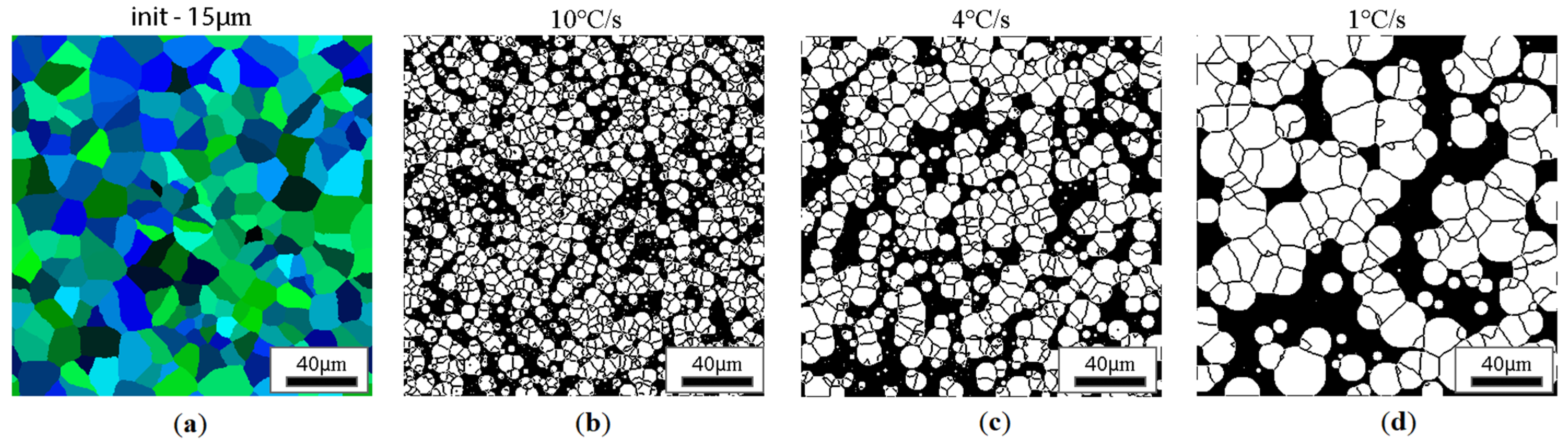
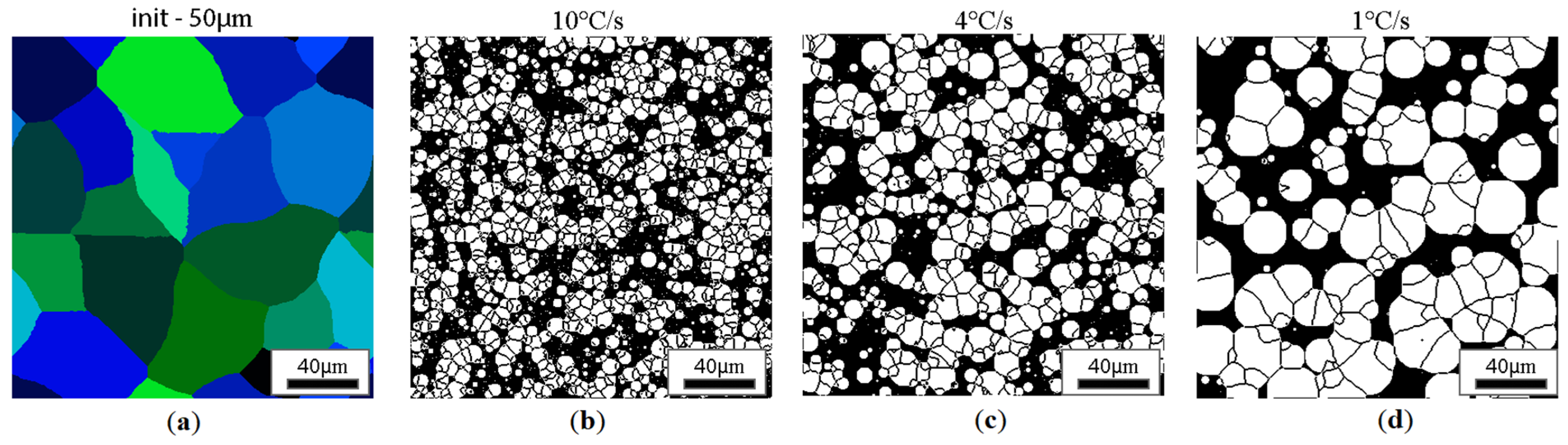
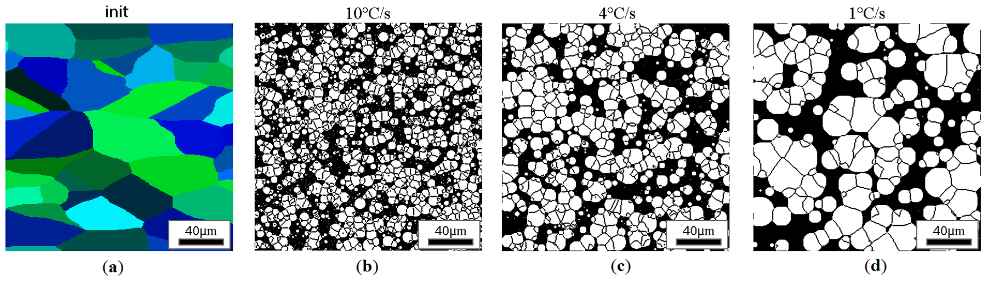
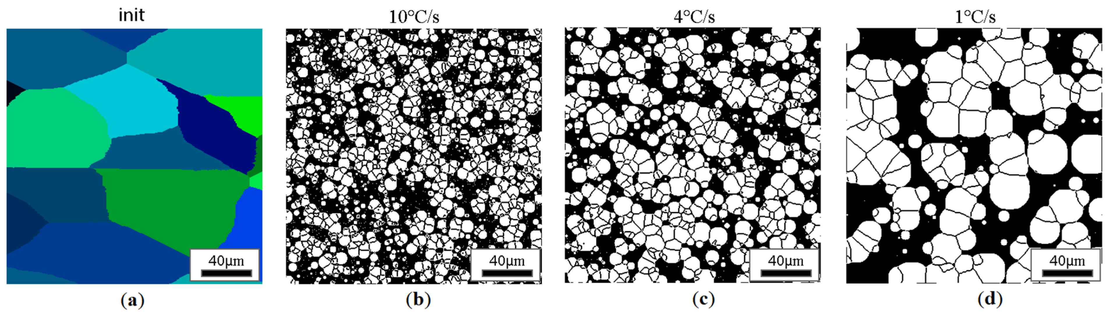
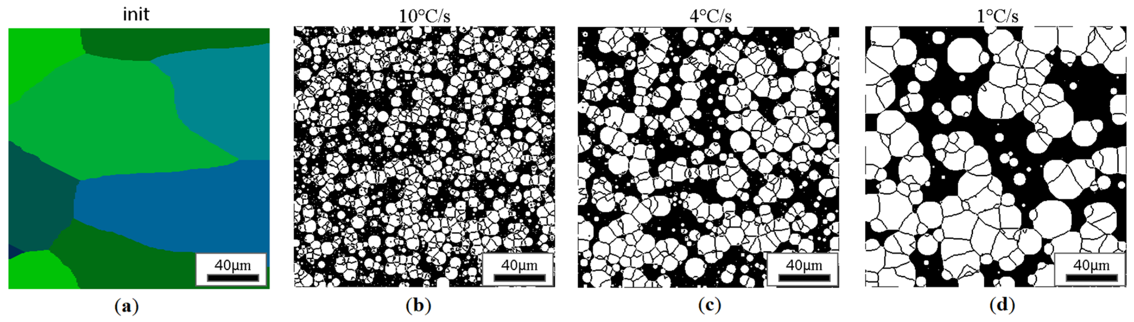
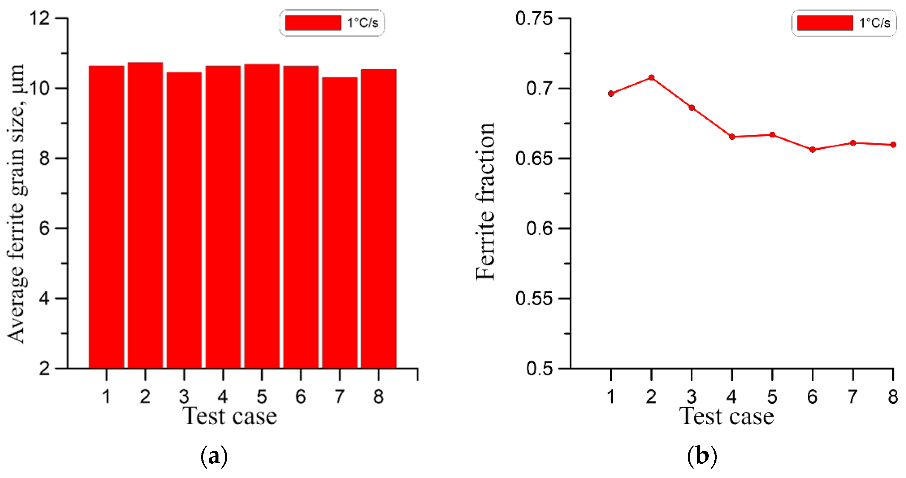
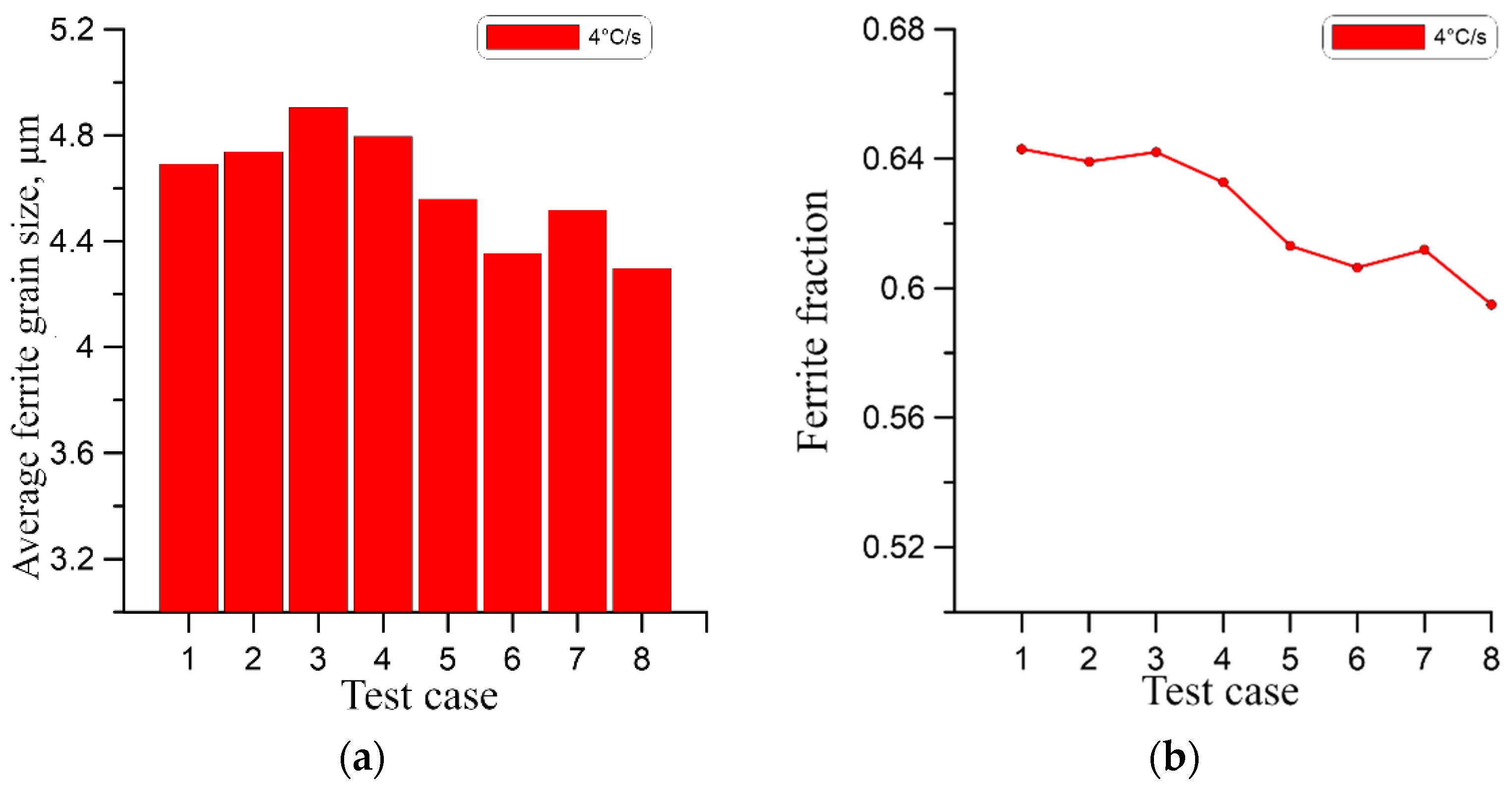
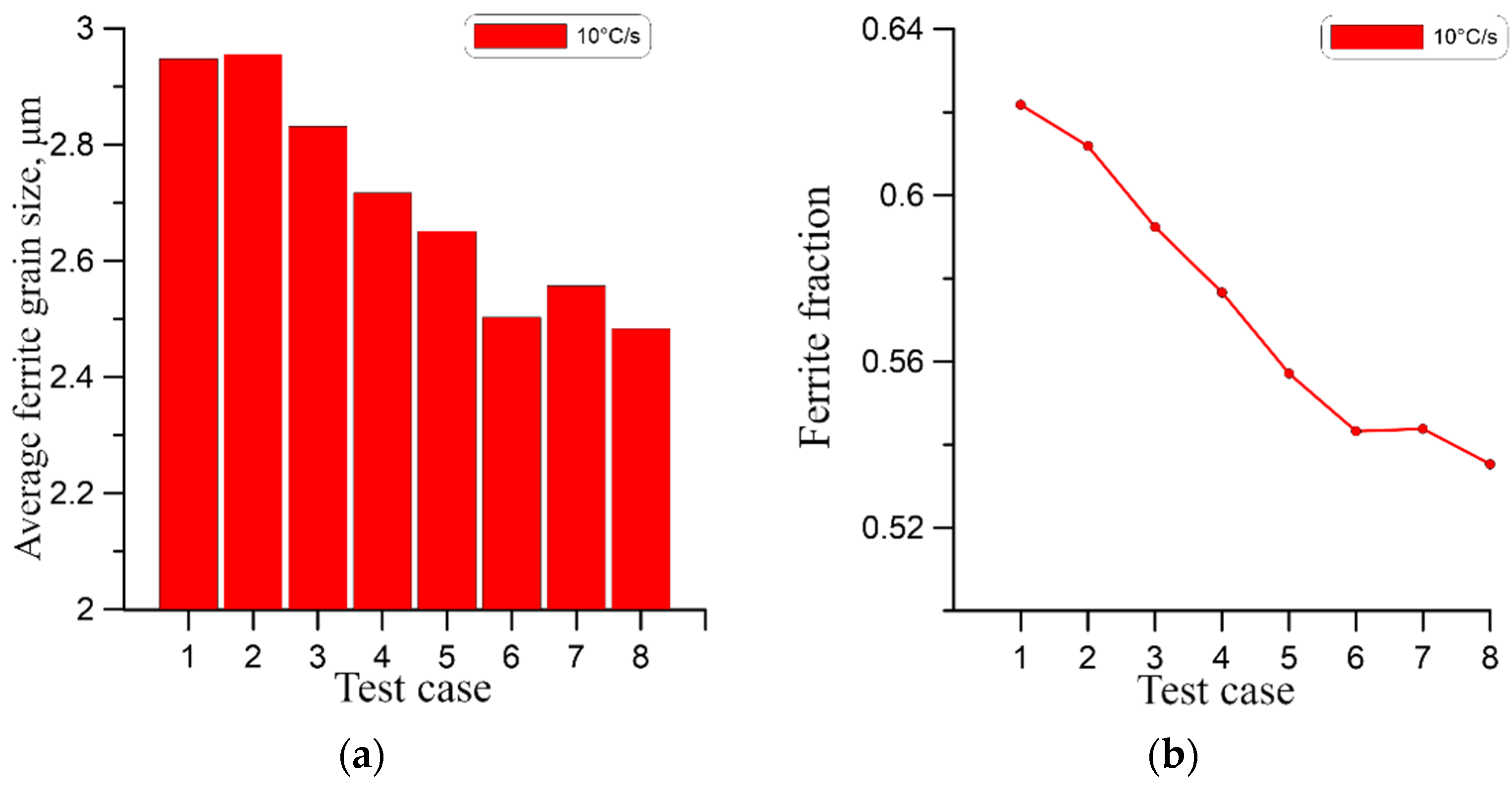
| Test Case No. | Initial Grain Size | Analysed Cooling Rate |
|---|---|---|
| 1 | 15 μm | 1, 4, 10 °C/s |
| 2 | 15 μm elongated 2× | 1, 4, 10 °C/s |
| 3 | 25 μm | 1, 4, 10 °C/s |
| 4 | 25 μm elongated 2× | 1, 4, 10 °C/s |
| 5 | 50 μm | 1, 4, 10 °C/s |
| 6 | 50 μm elongated 2× | 1, 4, 10 °C/s |
| 7 | 85 μm | 1, 4, 10 °C/s |
| 8 | 85 μm elongated 2× | 1, 4, 10 °C/s |
Disclaimer/Publisher’s Note: The statements, opinions and data contained in all publications are solely those of the individual author(s) and contributor(s) and not of MDPI and/or the editor(s). MDPI and/or the editor(s) disclaim responsibility for any injury to people or property resulting from any ideas, methods, instructions or products referred to in the content. |
© 2025 by the authors. Licensee MDPI, Basel, Switzerland. This article is an open access article distributed under the terms and conditions of the Creative Commons Attribution (CC BY) license (https://creativecommons.org/licenses/by/4.0/).
Share and Cite
Wermiński, M.; Sitko, M.; Madej, L. Through-Scale Numerical Investigation of Microstructure Evolution During the Cooling of Large-Diameter Rings. Materials 2025, 18, 3237. https://doi.org/10.3390/ma18143237
Wermiński M, Sitko M, Madej L. Through-Scale Numerical Investigation of Microstructure Evolution During the Cooling of Large-Diameter Rings. Materials. 2025; 18(14):3237. https://doi.org/10.3390/ma18143237
Chicago/Turabian StyleWermiński, Mariusz, Mateusz Sitko, and Lukasz Madej. 2025. "Through-Scale Numerical Investigation of Microstructure Evolution During the Cooling of Large-Diameter Rings" Materials 18, no. 14: 3237. https://doi.org/10.3390/ma18143237
APA StyleWermiński, M., Sitko, M., & Madej, L. (2025). Through-Scale Numerical Investigation of Microstructure Evolution During the Cooling of Large-Diameter Rings. Materials, 18(14), 3237. https://doi.org/10.3390/ma18143237