
Investigating the Effects of Surface Texture Direction and Poisson’s Ratio on Stress Concentration Factors


Abstract
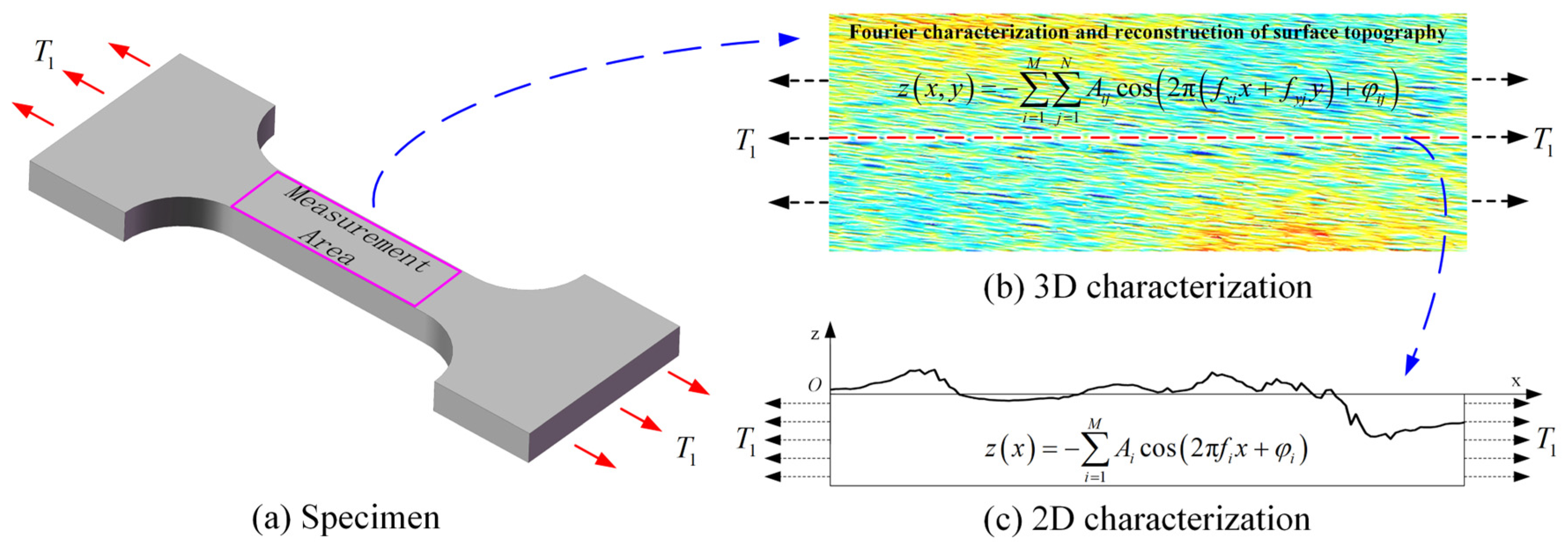
1. Introduction
2. General Analytical Solutions for SCFs
3. Analytical Solutions for Representative Geometric Surfaces
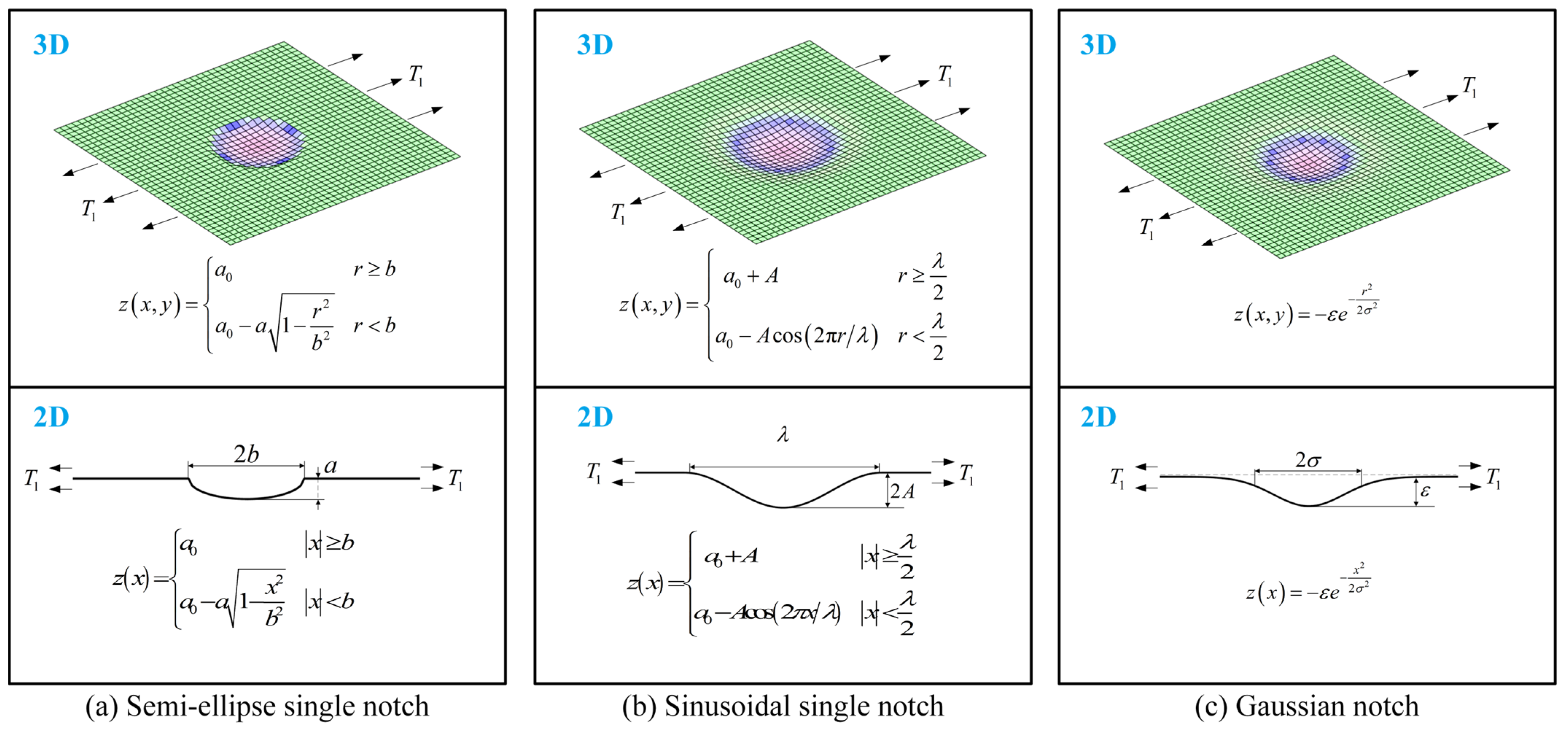
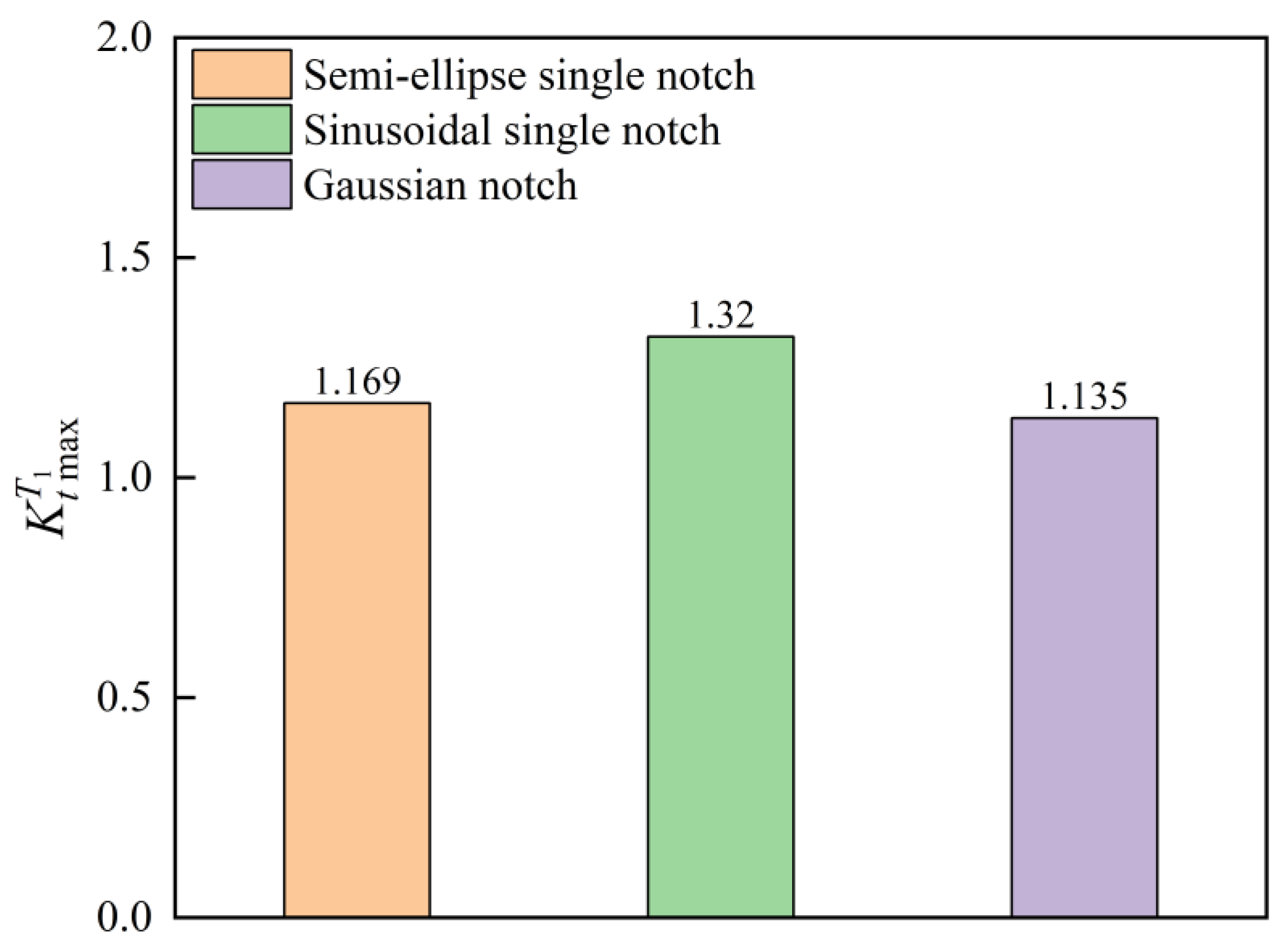
3.1. Single-Notch Geometric Surfaces
- (1)
- A semi-ellipse single notch
- (2)
- A sinusoidal single notch
- (3)
- A Gaussian notch
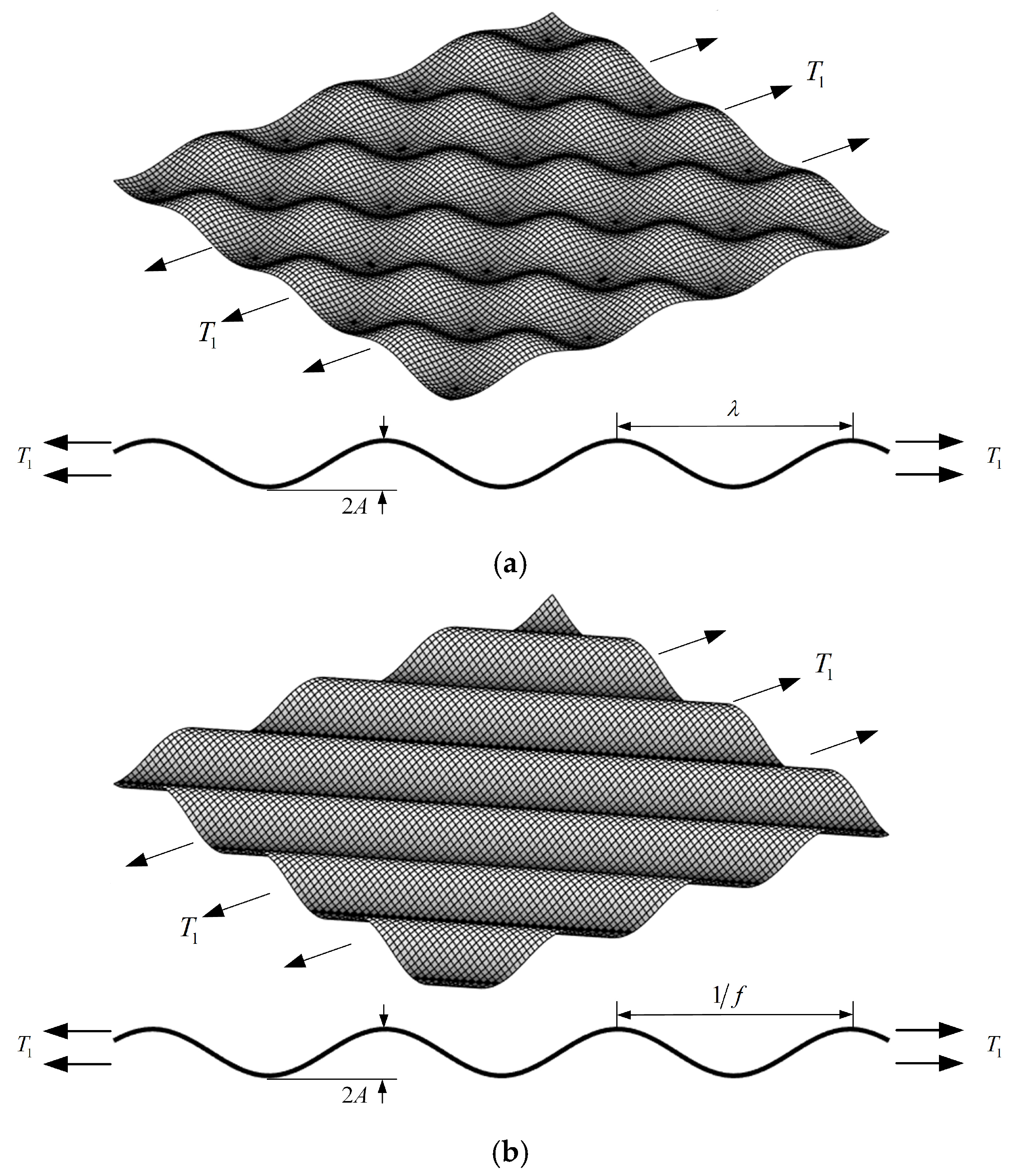
3.2. Single-Layer Cosine-Wave Surfaces
4. Finite Element Validation
4.1. Establishment of FEM
4.2. The Influence of Surface Texture Direction on SCFs
4.3. The Influence of Poisson’s Ratio on SCFs
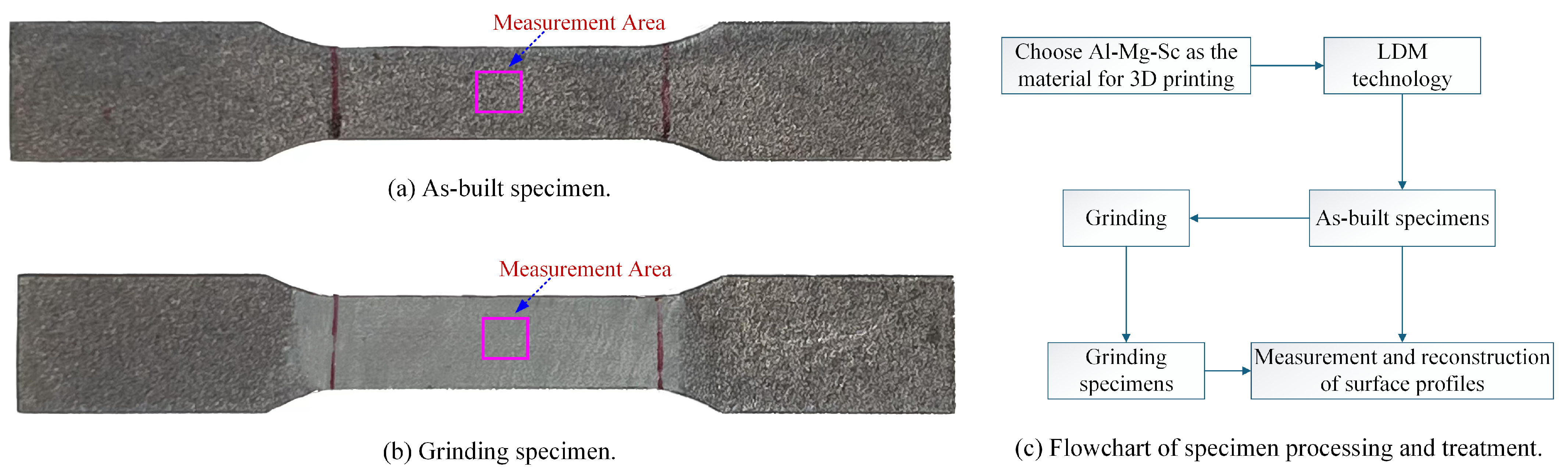
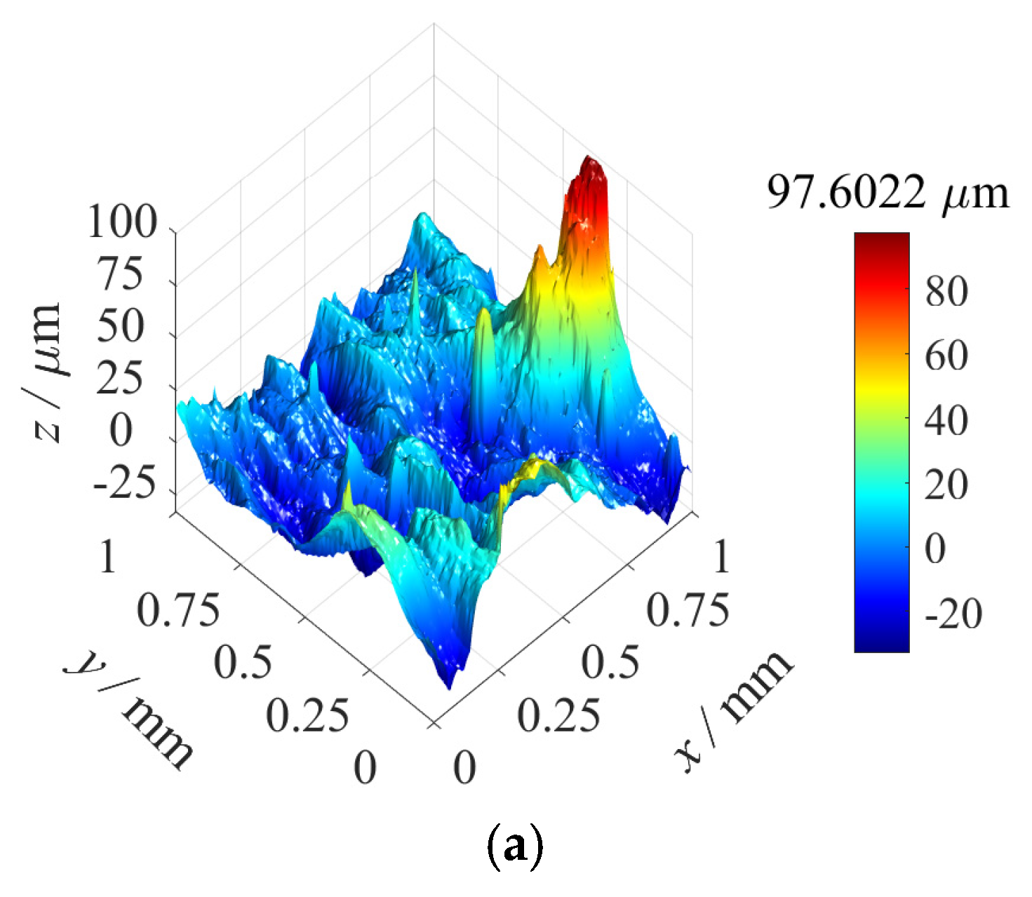
5. Application to Real Measured Surfaces
6. Conclusions
- (1)
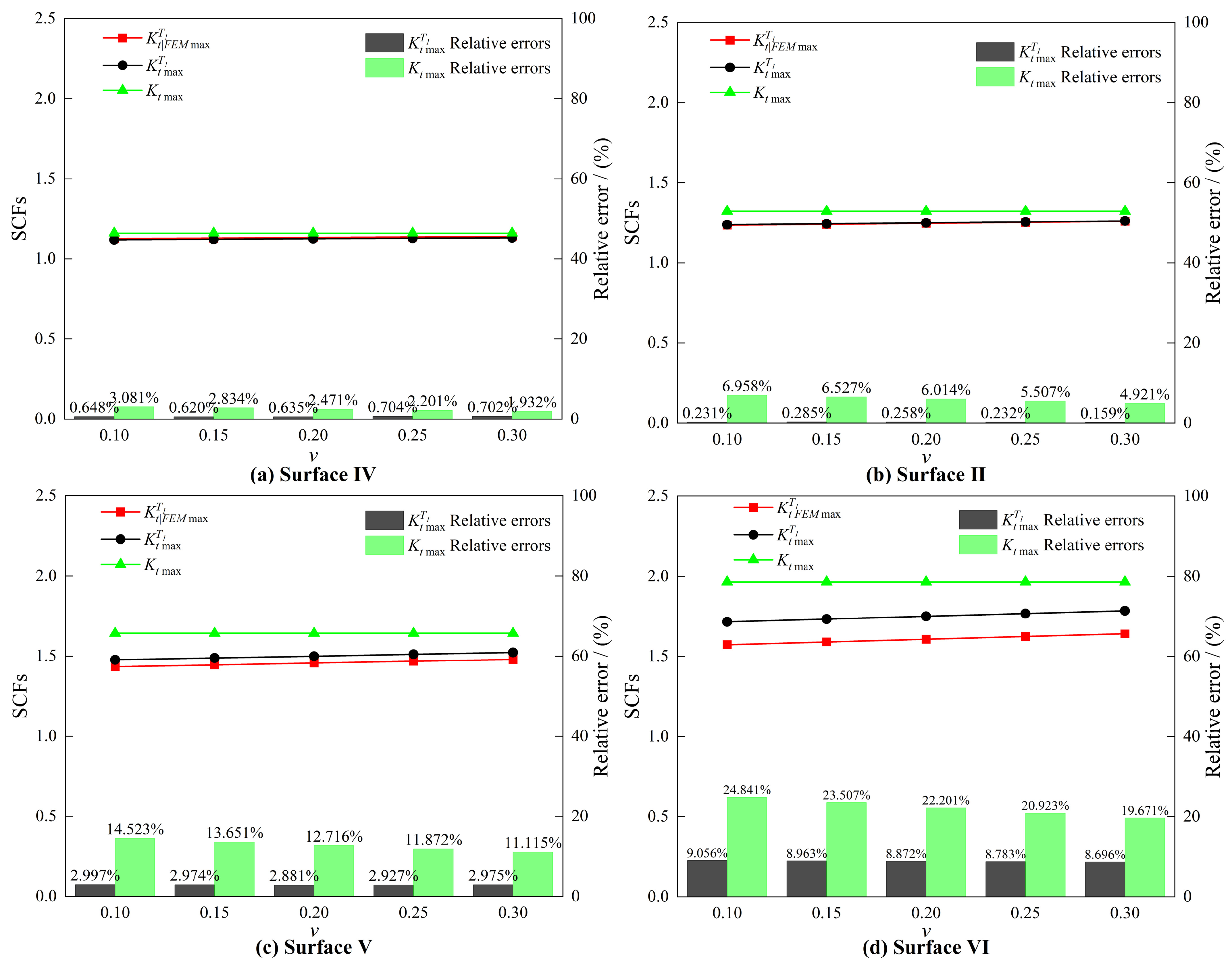
- Influence of Poisson’s ratio: The proposed 3D analytical solution distinctly reveals a positive correlation between and SCFs. This correlation represents a significant finding that conventional 2D models fail to capture.
- (2)
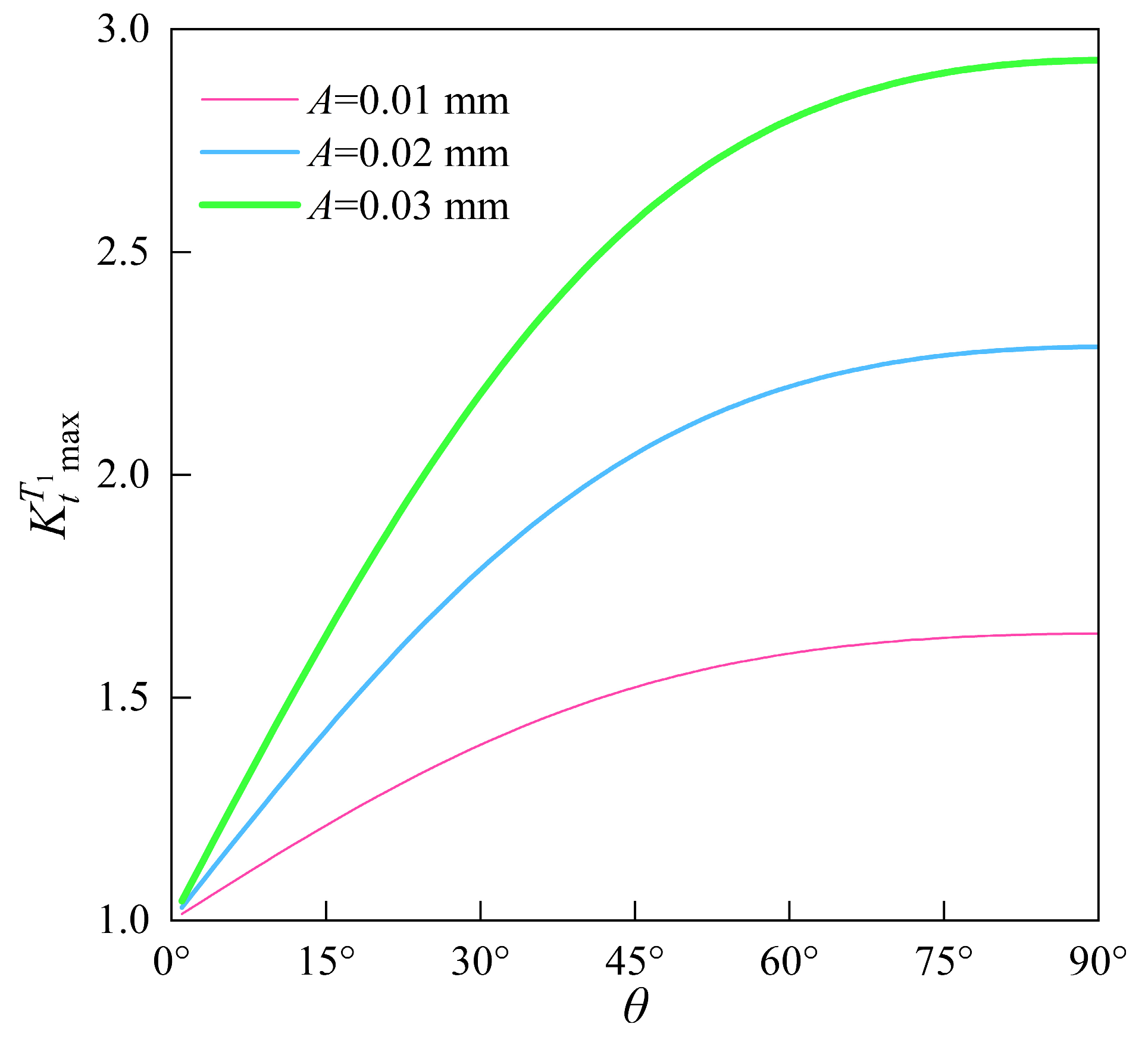
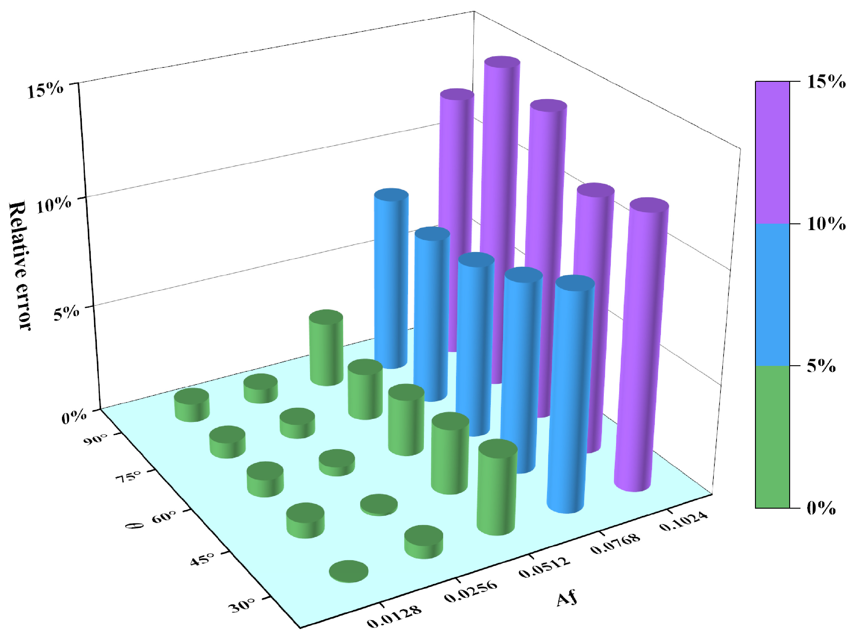
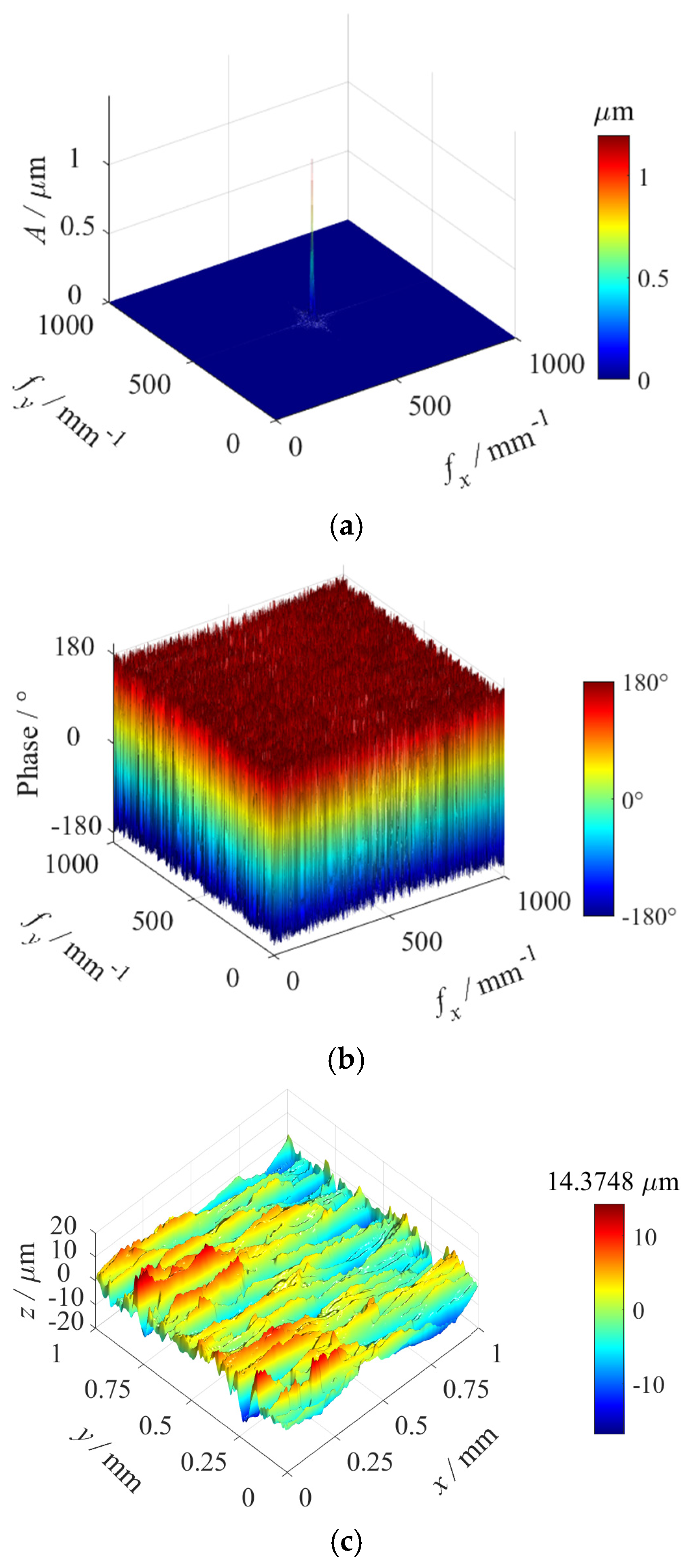
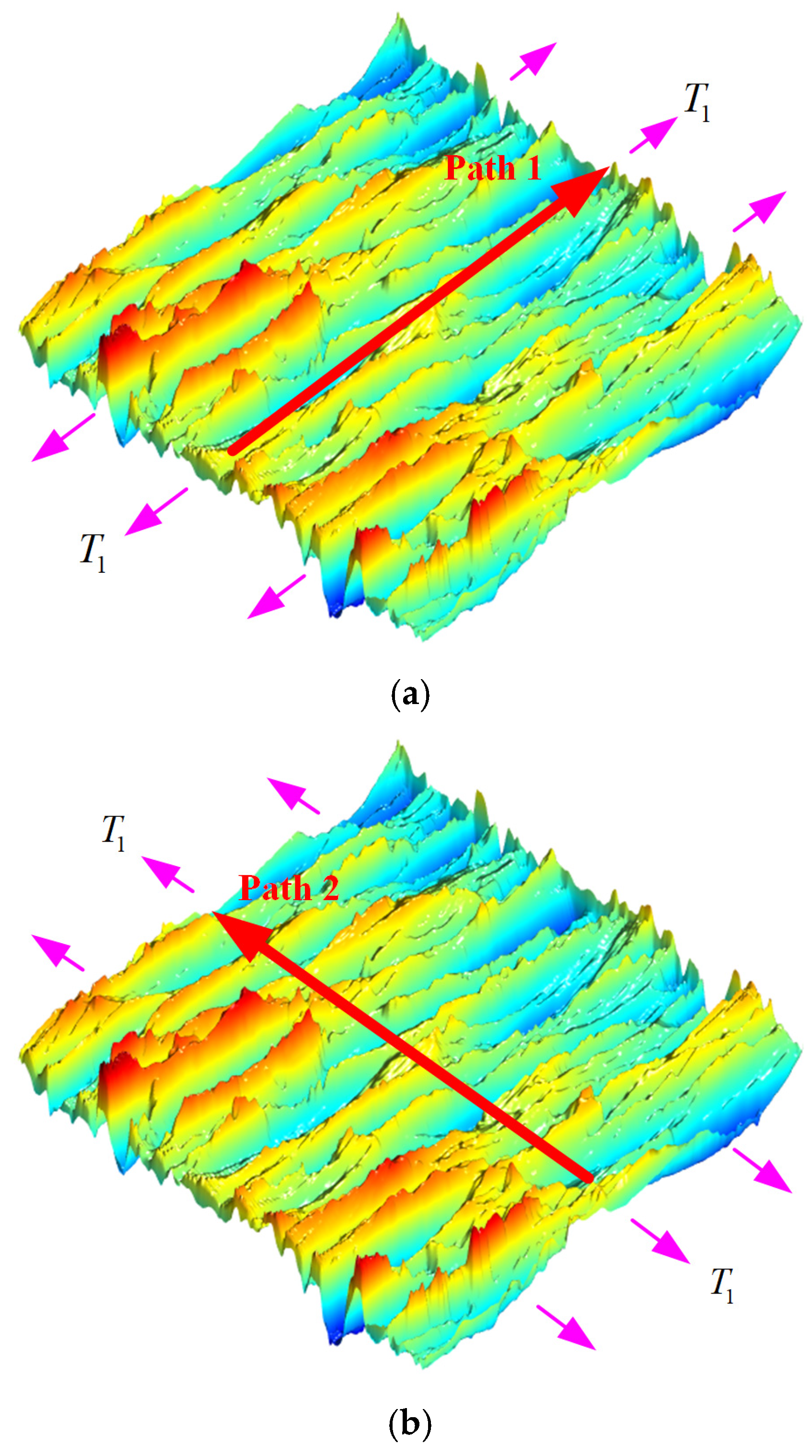
- Influence of texture directionality: Non-orthogonal surface textures exhibit remarkable anisotropic stress modulation, which is governed by the texture directional parameter . The 3D analytical solution quantitatively captures the phenomenon where SCFs increase monotonically with . In contrast, 2D solutions are unable to account for this directional sensitivity. A parametric analysis of single-layer cosine-wave surfaces further confirms a nonlinear relationship between the amplitude–frequency product and theoretical accuracy.
- (3)
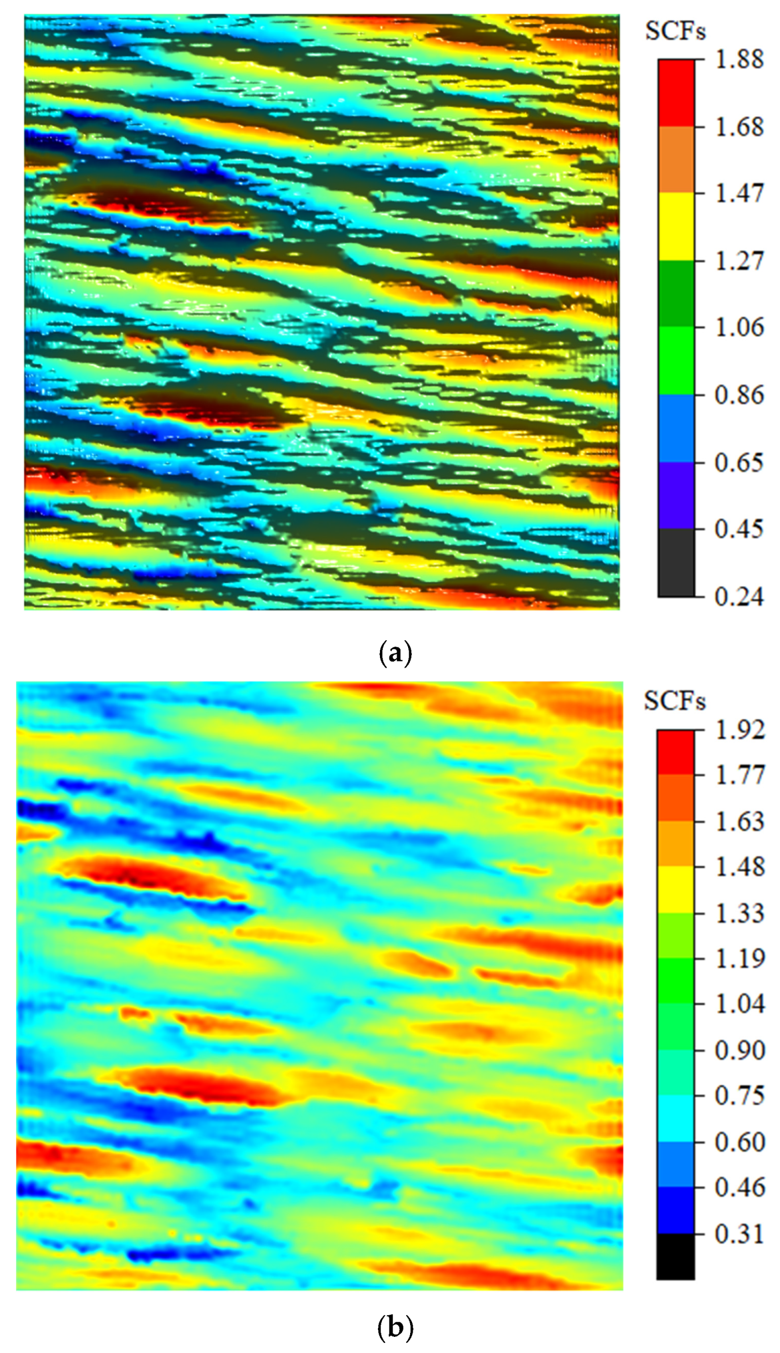
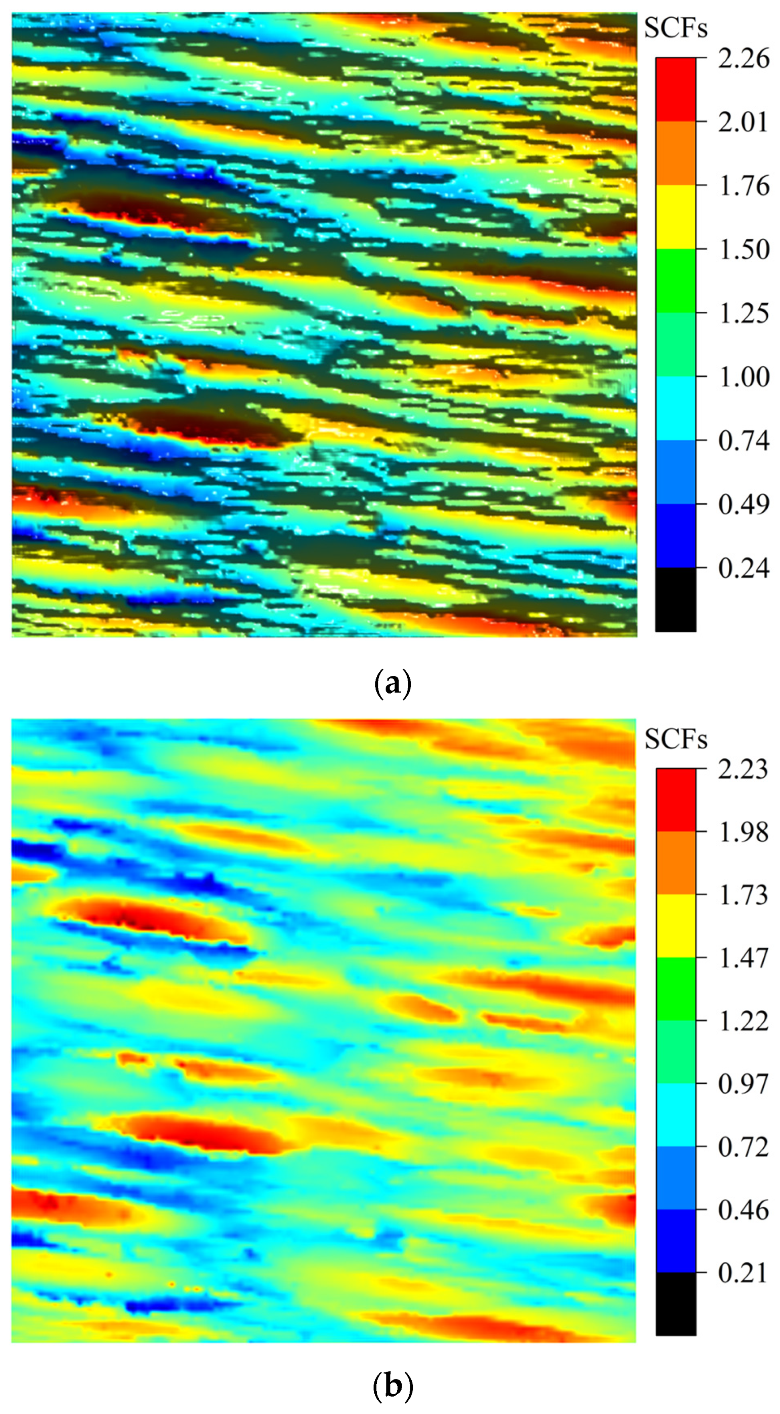
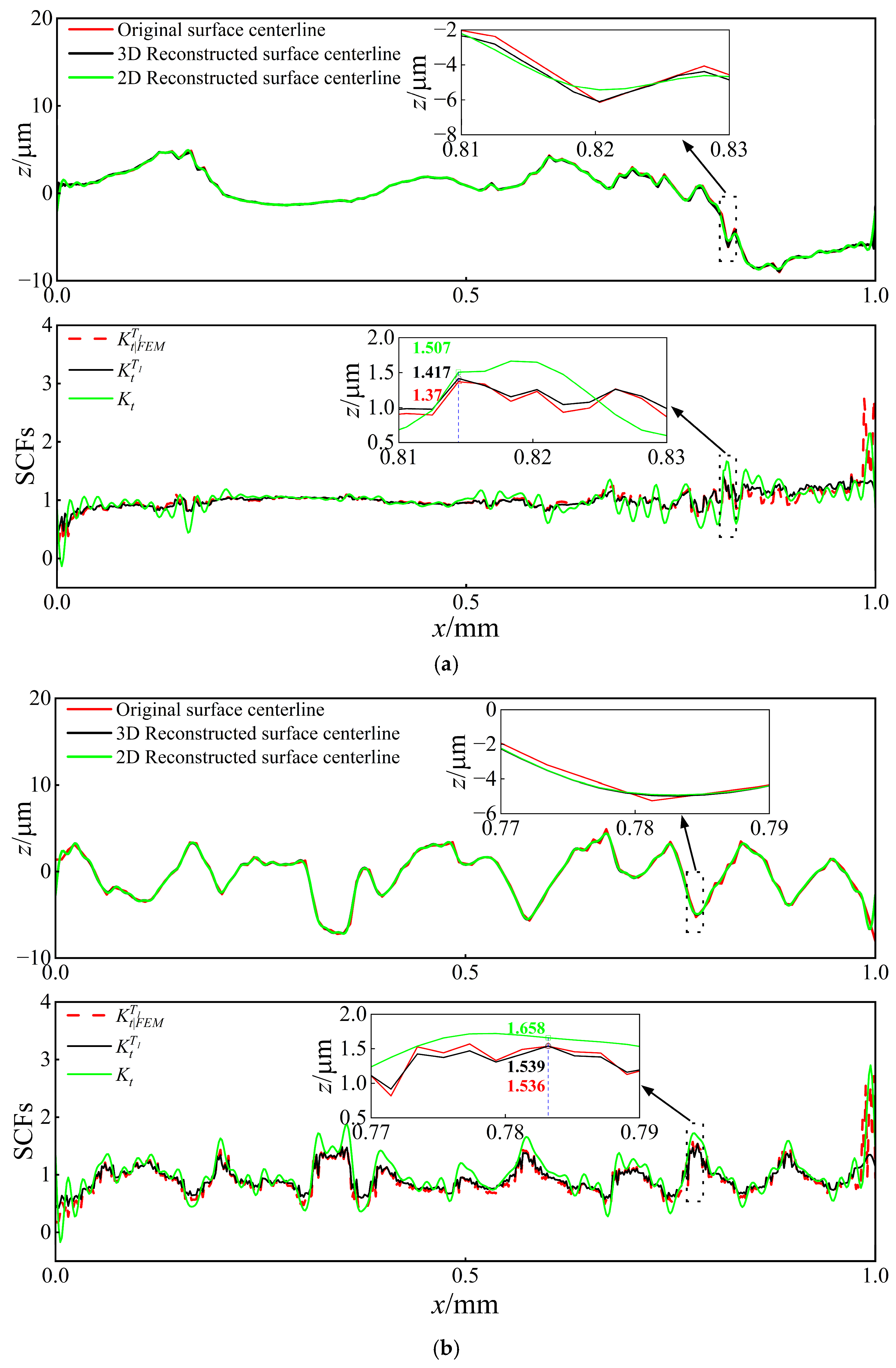
- Validation with real surface morphologies: Application to machined surfaces demonstrates the superior predictive capability of the 3D solution, achieving an average of 10% higher accuracy in SCF prediction compared to 2D methods, with relative errors stably maintained within 5%. The analysis further verifies that SCFs increase with increasing and are highly sensitive to surface texture directionality.
Author Contributions
Funding
Informed Consent Statement
Data Availability Statement
Acknowledgments
Conflicts of Interest
Nomenclature
| Notch depth of semi-ellipse notch | |
| / | Amplitude for sinusoidal and single-layer cosine wave/Gaussian notch |
| / | Amplitudes of the surface wave components in 2D/3D case |
| Notch half-width of semi-ellipse notch | |
| Loading ratio | |
| Surface frequency for single-layer cosine wave | |
| Surface frequency along direction | |
| / | Frequencies of the surface wave components in 2D/3D case |
| Kernel functions | |
| Analytical solution of normal SCFs in 2D case | |
| Analytical solution of normal SCFs in 3D case | |
| SCFs from finite element simulation results | |
| Maximum value of the analytical solution for 2D SCFs | |
| Maximum value of the analytical solution for 3D SCFs | |
| Maximum SCFs from finite element simulation results | |
| Analytical solution of shear SCFs in 3D case | |
| The maximum stress perturbation ratio | |
| Distance between two points | |
| The arithmetic mean height parameter | |
| Loading | |
| Poisson’s ratio | |
| Two-dimensional surface profile | |
| Three-dimensional surface topography | |
| Height matrix | |
| The standard deviation | |
| Displacement and stress | |
| / | Phases of the surface wave components in 2D/3D case |
| Wavelength parameter | |
| The coefficient | |
| Texture direction parameter |
References
- Stephens, R.I.; Fatemi, A.; Stephens, R.R.; Fuchs, H.O. Metal Fatigue in Engineering; John Wiley & Sons: Hoboken, NJ, USA, 2000. [Google Scholar]
- Juoksukangas, J.; Nurmi, V.; Hintikka, J.; Vippola, M.; Lehtovaara, A.; Mäntylä, A.; Vaara, J.; Frondelius, T. Characterization of cracks formed in large flat-on-flat fretting contact. Int. J. Fatigue 2019, 124, 361–370. [Google Scholar] [CrossRef]
- Azevedo, T.F.; Lima, T.N.; Macedo, M.D.; de Blas, J.G.; Griza, S. Fracture mechanics behavior of TiNbSn alloys as a function of alloy content, cold working and aging. Eng. Fract. Mech. 2020, 229, 106946. [Google Scholar] [CrossRef]
- Becker, N.; Tunsch, P.; Ulrich, C.; Schlecht, B. Surface roughness measurement in the notch area for estimating dynamic component load bearing capacity. Forsch. Im Ingenieurwesen 2024, 88, 37. [Google Scholar] [CrossRef]
- Zerbst, U.; Madia, M.; Klinger, C.; Bettge, D.; Murakami, Y. Defects as a root cause of fatigue failure of metallic components. III: Cavities, dents, corrosion pits, scratches. Eng. Fail. Anal. 2019, 97, 759–776. [Google Scholar] [CrossRef]
- Murakami, Y. Metal Fatigue: Effects of Small Defects and Nonmetallic Inclusions; Academic Press: Cambridge, MA, USA, 2019. [Google Scholar]
- Luo, D.; Wang, Y.; Wang, F.; Cheng, H.; Zhang, B.; Zhu, Y. The influence of metal cover plates on ballistic performance of silicon carbide subjected to large-scale tungsten projectile. Mater. Des. 2020, 191, 108659. [Google Scholar] [CrossRef]
- Lee, J.-M.; Kim, Y.-J.; Kim, J.-W. Very low cycle fatigue life evaluation models and validation using notched compact tension test data. Int. J. Fatigue 2022, 155, 106635. [Google Scholar] [CrossRef]
- Zhang, Y.; Seveyrat, L.; Lebrun, L. Correlation between dielectric, mechanical properties and electromechanical performance of functionalized graphene/polyurethane nanocomposites. Compos. Sci. Technol. 2021, 211, 108843. [Google Scholar] [CrossRef]
- Vayssette, B.; Saintier, N.; Brugger, C.; El May, M.; Pessard, E. Numerical modelling of surface roughness effect on the fatigue behavior of Ti-6Al-4V obtained by additive manufacturing. Int. J. Fatigue 2019, 123, 180–195. [Google Scholar] [CrossRef]
- Lee, S.; Pegues, J.W.; Shamsaei, N. Fatigue behavior and modeling for additive manufactured 304L stainless steel: The effect of surface roughness. Int. J. Fatigue 2020, 141, 105856. [Google Scholar] [CrossRef]
- Nedele, M.R.; Wisnom, M.R. Three-dimensional finite element analysis of the stress concentration at a single fibre break. Compos. Sci. Technol. 1994, 51, 517–524. [Google Scholar] [CrossRef]
- Kubair, D.V.; Bhanu-Chandar, B. Stress concentration factor due to a circular hole in functionally graded panels under uniaxial tension. Int. J. Mech. Sci. 2008, 50, 732–742. [Google Scholar] [CrossRef]
- Azar, A.S. Exploring the stress concentration factor in additively manufactured materials: A machine learning perspective on surface notches and subsurface defects. Theor. Appl. Fract. Mech. 2024, 130, 104298. [Google Scholar] [CrossRef]
- Kantzos, C.; Lao, J.; Rollett, A. Design of an interpretable Convolutional Neural Network for stress concentration prediction in rough surfaces. Mater. Charact. 2019, 158, 109961. [Google Scholar] [CrossRef]
- Liu, H.; Zhang, Y. Image-driven structural steel damage condition assessment method using deep learning algorithm. Measurement 2019, 133, 168–181. [Google Scholar] [CrossRef]
- Sanaei, N.; Fatemi, A. Analysis of the effect of surface roughness on fatigue performance of powder bed fusion additive manufactured metals. Theor. Appl. Fract. Mech. 2020, 108, 102638. [Google Scholar] [CrossRef]
- Romano, S.; Nezhadfar, P.D.; Shamsaei, N.; Seifi, M.; Beretta, S. High cycle fatigue behavior and life prediction for additively manufactured 17-4 PH stainless steel: Effect of sub-surface porosity and surface roughness. Theor. Appl. Fract. Mech. 2020, 106, 102477. [Google Scholar] [CrossRef]
- Cheng, Z.; Zhu, X.; Zhang, Y.; Wang, T.; Berto, F. Analytical prediction of the fatigue limit for axisymmetric round bars with rough surface morphology. Fatigue Fract. Eng. Mater. Struct. 2021, 45, 739–753. [Google Scholar] [CrossRef]
- Sombatmai, A.; Uthaisangsuk, V.; Wongwises, S.; Promoppatum, P. Multiscale investigation of the influence of geometrical imperfections, porosity, and size-dependent features on mechanical behavior of additively manufactured Ti-6Al-4V lattice struts. Mater. Des. 2021, 209, 109985. [Google Scholar] [CrossRef]
- Yang, C.; Bian, H.; Zhang, F.; Cui, Y.; Lei, Y.; Hayasaka, Y.; Aoyagi, K.; Yamanaka, K.; Chiba, A. Competition between solid solution and multi-component Laves phase in a dual-phase refractory high-entropy alloy CrHfNbTaTi. Mater. Des. 2023, 226, 111646. [Google Scholar] [CrossRef]
- Shrestha, R.; Simsiriwong, J.; Shamsaei, N. Fatigue behavior of additive manufactured 316L stainless steel parts: Effects of layer orientation and surface roughness. Addit. Manuf. 2019, 28, 23–38. [Google Scholar] [CrossRef]
- Lee, S.; Shao, S.; Wells, D.N.; Zetek, M.; Kepka, M.; Shamsaei, N. Fatigue behavior and modeling of additively manufactured IN718: The effect of surface treatments and surface measurement techniques. J. Mater. Process. Technol. 2022, 302, 117475. [Google Scholar] [CrossRef]
- Schneller, W.; Leitner, M.; Pomberger, S.; Grün, F.; Leuders, S.; Pfeifer, T.; Jantschner, O. Fatigue strength assessment of additively manufactured metallic structures considering bulk and surface layer characteristics. Addit. Manuf. 2021, 40, 101930. [Google Scholar] [CrossRef]
- Arola, D.; Williams, C. Estimating the fatigue stress concentration factor of machined surfaces. Int. J. Fatigue 2002, 24, 923–930. [Google Scholar] [CrossRef]
- Marvin Luna, V.; Kim, I.-T.; Jeong, Y.-S. Stress concentration factor estimation for corroded steel plates using the surface gradient method. Eng. Fail. Anal. 2024, 163, 108509. [Google Scholar] [CrossRef]
- Yan, X. An empirical formula for stress intensity factors of cracks emanating from a circular hole in a rectangular plate in tension. Eng. Fail. Anal. 2007, 14, 935–940. [Google Scholar] [CrossRef]
- Choi, S.-H.; Kim, D.; Park, S.; You, B. Simulation of stress concentration in Mg alloys using the crystal plasticity finite element method. Acta Mater. 2010, 58, 320–329. [Google Scholar] [CrossRef]
- Dobson, T.; Larrosa, N.; Coules, H. The role of corrosion pit topography on stress concentration. Eng. Fail. Anal. 2024, 157, 107900. [Google Scholar] [CrossRef]
- Guo, X.; Yan, Z.; Yu, J. Failure analysis of kingpin hole on front axle of mining truck based on finite element analysis. Eng. Fail. Anal. 2024, 166, 108888. [Google Scholar] [CrossRef]
- Zhang, J.; Chen, H.; Fu, H.; Cui, Y.; Wang, C.; Chen, H.; Yang, Z.; Cao, W.; Liang, J.; Zhang, C. Retarding effect of submicron carbides on short fatigue crack propagation: Mechanistic modeling and Experimental validation. Acta Mater. 2023, 250, 118875. [Google Scholar] [CrossRef]
- Lizarazu, J.; Harirchian, E.; Shaik, U.A.; Shareef, M.; Antoni-Zdziobek, A.; Lahmer, T. Application of machine learning-based algorithms to predict the stress-strain curves of additively manufactured mild steel out of its microstructural characteristics. Results Eng. 2023, 20, 101587. [Google Scholar] [CrossRef]
- Neuber, H. Kerbspannungslehre: Theorie der Spannungskonzentration Genaue Berechnung der Festigkeit; Springer: Berlin/Heidelberg, Germany, 2013. [Google Scholar]
- Arola, D.; Ramulu, M.; Arola, D.M.R. An Examination of the Effects from Surface Texture on the Strength of Fiber Reinforced Plastics. J. Compos. Mater. 1999, 33, 102–123. [Google Scholar] [CrossRef]
- Gu, H.; Jiao, L.; Yan, P.; Guo, Z.; Qiu, T.; Wang, X. A Surface Skewness and Kurtosis Integrated Stress Concentration Factor Model. J. Tribol. 2023, 145, 041702. [Google Scholar] [CrossRef]
- Rodrigues, M.A.C.; Burgos, R.B.; Martha, L.F. A unified approach to the Timoshenko 3D beam-column element tangent stiffness matrix considering higher-order terms in the strain tensor and large rotations. Int. J. Solids Struct. 2021, 222–223, 111003. [Google Scholar]
- Qin, J.; Huang, H.; Xie, Y.; Pan, S.; Chen, Y.; Yang, L.; Jiang, Q.; He, H. MXene supported rhodium nanocrystals for efficient electrocatalysts towards methanol oxidation. Ceram. Int. 2022, 48, 15327–15333. [Google Scholar] [CrossRef]
- Lee, S.; Rasoolian, B.; Silva, D.F.; Pegues, J.W.; Shamsaei, N. Surface roughness parameter and modeling for fatigue behavior of additive manufactured parts: A non-destructive data-driven approach. Addit. Manuf. 2021, 46, 102094. [Google Scholar] [CrossRef]
- Dinh, T.D.; Han, S.; Yaghoubi, V.; Xiang, H.; Erdelyi, H.; Craeghs, T.; Segers, J.; Van Paepegem, W. Modeling detrimental effects of high surface roughness on the fatigue behavior of additively manufactured Ti-6Al-4V alloys. Int. J. Fatigue 2021, 144, 106034. [Google Scholar] [CrossRef]
- Gao, H. Stress concentration at slightly undulating surfaces. J. Mech. Phys. Solids 1991, 39, 443–458. [Google Scholar] [CrossRef]
- Medina, H.; Hinderliter, B. The stress concentration factor for slightly roughened random surfaces: Analytical solution. Int. J. Solids Struct. 2014, 51, 2012–2018. [Google Scholar] [CrossRef]
- Cheng, Z.; Liao, R.; Lu, W. Surface stress concentration factor via Fourier representation and its application for machined surfaces. Int. J. Solids Struct. 2017, 113, 108–117. [Google Scholar] [CrossRef]
- Persson, B.N.J. Surface Roughness-Induced Stress Concentration. Tribol. Lett. 2023, 71, 66. [Google Scholar] [CrossRef]
- Cheng, Z.; Zhang, Y.; Sun, X.; Wang, T.; Li, S. Stress concentration of 3-D surfaces with small undulations: Analytical solution. Int. J. Solids Struct. 2020, 206, 340–353. [Google Scholar] [CrossRef]
- Perez, I.; Madariaga, A.; Arrazola, P.J.; Cuesta, M.; Soriano, D. An analytical approach to calculate stress concentration factors of machined surfaces. Int. J. Mech. Sci. 2021, 190, 106040. [Google Scholar] [CrossRef]
- Medina, H. A stress-concentration-formula generating equation for arbitrary shallow surfaces. Int. J. Solids Struct. 2015, 69–70, 86–93. [Google Scholar] [CrossRef]
- Cheng, Z.; Liao, R.; Lu, W.; Wang, D. Fatigue notch factors prediction of rough specimen by the theory of critical distance. Int. J. Fatigue 2017, 104, 195–205. [Google Scholar] [CrossRef]
- Toyoda, S.; Kawabata, Y.; Sakata, K.; Sato, A.; Yoshihara, N.; Sakai, J.I. Estimating the Effects of Microscopic Stress Concentrations on the Fatigue Endurance of Thin-walled High Strength Steel. ISIJ Int. 2009, 49, 1806–1813. [Google Scholar] [CrossRef]
- Chen, S.; Zhao, W.; Yan, P.; Qiu, T.; Gu, H.; Jiao, L.; Wang, X. Effect of milling surface topography and texture direction on fatigue behavior of ZK61M magnesium alloy. Int. J. Fatigue 2022, 156, 106669. [Google Scholar] [CrossRef]


| 30° | 45° | 60° | 75° | 90° | ||
|---|---|---|---|---|---|---|
| 0.0128 | 1.098 | 1.139 | 1.159 | 1.167 | 1.171 | |
| 1.099 | 1.131 | 1.15 | 1.584 | 1.161 | ||
| 0.0256 | 1.190 | 1.260 | 1.294 | 1.326 | 1.331 | |
| 1.197 | 1.262 | 1.299 | 1.317 | 1.322 | ||
| 0.0512 | 1.347 | 1.479 | 1.558 | 1.599 | 1.695 | |
| 1.394 | 1.523 | 1.599 | 1.634 | 1.643 | ||
| 0.0768 | 1.439 | 1.642 | 1.759 | 1.811 | 1.816 | |
| 1.591 | 1.785 | 1.899 | 1.951 | 1.965 | ||
| 0.1024 | 1.592 | 1.833 | 1.927 | 1.975 | 2.037 | |
| 1.788 | 2.046 | 2.198 | 2.268 | 2.287 | ||
by Equation (35) | by Equation (37) | Relative Errors of 3D Analytical Solution | Relative Errors of 2D Analytical Solution | ||
|---|---|---|---|---|---|
| 0.1 | 1.350 | 1.386 | 1.507 | 2.64% | 11.63% |
| 0.15 | 1.355 | 1.390 | 2.55% | 11.22% | |
| 0.2 | 1.359 | 1.392 | 2.45% | 10.89% | |
| 0.25 | 1.365 | 1.397 | 2.34% | 10.40% | |
| 0.3 | 1.370 | 1.417 | 3.44% | 10.00% |
Disclaimer/Publisher’s Note: The statements, opinions and data contained in all publications are solely those of the individual author(s) and contributor(s) and not of MDPI and/or the editor(s). MDPI and/or the editor(s) disclaim responsibility for any injury to people or property resulting from any ideas, methods, instructions or products referred to in the content. |
© 2025 by the authors. Licensee MDPI, Basel, Switzerland. This article is an open access article distributed under the terms and conditions of the Creative Commons Attribution (CC BY) license (https://creativecommons.org/licenses/by/4.0/).
Share and Cite
Liu, Y.; Liu, Y.; Cheng, Z. Investigating the Effects of Surface Texture Direction and Poisson’s Ratio on Stress Concentration Factors. Materials 2025, 18, 2260. https://doi.org/10.3390/ma18102260
Liu Y, Liu Y, Cheng Z. Investigating the Effects of Surface Texture Direction and Poisson’s Ratio on Stress Concentration Factors. Materials. 2025; 18(10):2260. https://doi.org/10.3390/ma18102260
Chicago/Turabian StyleLiu, Yuwei, Yuhui Liu, and Zhengkun Cheng. 2025. "Investigating the Effects of Surface Texture Direction and Poisson’s Ratio on Stress Concentration Factors" Materials 18, no. 10: 2260. https://doi.org/10.3390/ma18102260
APA StyleLiu, Y., Liu, Y., & Cheng, Z. (2025). Investigating the Effects of Surface Texture Direction and Poisson’s Ratio on Stress Concentration Factors. Materials, 18(10), 2260. https://doi.org/10.3390/ma18102260