Abstract
The convolution of two physical entities, denoted as f and g, delineates the manner in which one entity undergoes modification in response to the other. This transformative process is mathematically represented by the expression f ⨂ g, symbolizing the convolution of the two entities in a resultant function h. Frequently, it becomes imperative to comprehend the magnitude of the induced modifications. From the derived function h, a crucial step involves the separation of the two original signals, a process commonly referred to as deconvolution. Various techniques have been proposed to facilitate the calculation of the deconvolution, with one notable approach originating in 1931 by van Cittert. The algorithm, based on an iterative method, has been scrutinized over time, notably by Bracewell and, more recently, by Jansson. This work represents the current state-of-the-art, focusing specifically on the analysis of Auger spectra obtained through XPS. Emphasis is placed on delineating the procedural aspects of the analysis, and the algorithm utilized in the open-source software RxpsG is comprehensively described.
1. Introduction
Interference among data poses a common challenge across various spectroscopic techniques. An illustrative instance is the signal overlap encountered in astronomy, necessitating the application of deblurring techniques for the removal of atmospheric effects from observed signals through deconvolution methods [1]. Similarly, deconvolution proves important in mitigating turbulence effects within data acquired from diverse engineering and geophysical systems, spanning a broad spectrum of spatial and temporal scales [2]. Although resolving such issues through numerical simulations which can describe local motion features is conceivable, the associated computational effort becomes prohibitive. Consequently, deconvolution techniques are employed to alleviate computational load while upholding a comprehensive system description. Another noteworthy application of deconvolution is the analysis of strain maps derived from materials subjected to mechanical testing [3]. Deconvolution is explored in this context to mitigate noise and recover the actual displacement and strain fields from localized digital image correlation maps or localized spectrum analyses. This underscores the pivotal role played by deconvolution in enhancing the fidelity of data interpretation and analysis in diverse scientific domains.
In addition to addressing noise, within the context of the current study, another prevalent scenario where deconvolution finds widespread application is in mitigating interference stemming from the contribution of distinct spectral lines. The challenge lies in the unknown intensity and position of these interfering lines, thereby complicating the reconstruction of the resultant spectrum [4]. Broadly, the experimental spectrum is seen as a convolution in the analysis, with the objective of enhancing resolution through deconvolution. This interpretation involves considering the experimental spectrum h as the convolution of the original line shape f with a function g. This function g represents the contribution of additional spectral lines, the source of spectral Gaussian broadening, or systematic instrumental broadening [5,6,7]. By adopting this perspective, the deconvolution process becomes integral to unraveling the complexities of the spectral data and discerning the underlying components contributing to the observed interference.
In this manuscript, we will illustrate the application of deconvolution in analyzing Auger spectra obtained through X-ray Photoelectron Spectroscopy (XPS). In XPS, X-photons are utilized to excite electrons to the vacuum level. The kinetic energy of the detected photoelectrons can be correlated with the orbital of the emitting atom, enabling speciation and quantification of element abundances. During photoemission, a valence electron may relax into the core hole created by X-excitation. The energy released can excite a second valence electron, known as the Auger electron, into the vacuum level.
The Auger spectra can be conceptualized as the self-convolution of two valence states: the first corresponds to the electron relaxing into the hole, and the second involves emission into the vacuum after absorbing the released energy. This process mixes all valence states, rendering the Auger spectrum as the self-convolution of the density of states (DOS). Consequently, analyzing Auger spectra offers valuable insights into the electronic structure of valence electrons, including spectral changes induced by chemical bonds [8,9,10]. Regrettably, the photoemission process is intricate, and the resulting spectra are the overlap of various processes. Core lines, originating from the direct absorption of an X-photon and emission from an inner level, and Auger spectra typically appear at well-separated kinetic energies. However, photoelectrons from core levels may lose part of their energy in exciting valence electrons, generating a loss features such as plasmons, shake-up, and shake-off structures [8,9]. As these features impact the electronic structure of valence electrons, Auger spectra are perturbed and cannot be acquired separately from the contributions due to their loss features. Because they affect the electronic structure of the valence electrons, their effect is convolved with the pure Auger spectrum.
So far, to obtain a clear description of the valence structure, it is necessary to deconvolve the effects of relaxation processes from the Auger spectrum. The scope of this manuscript is to provide a comprehensive overview of potential solutions for signal deconvolution. Deconvolving the loss features from the Auger spectrum will be used as an example to showcase the deconvolution process and highlight the solutions implemented in the RxpsG software (https://github.com/GSperanza accessed on 24 January 2024) for signal processing [11].
2. Analysis of the Auger Spectrum and the Van-Cittert Algorithm
The core–valence–valence Auger transitions involve the relaxation of a valence electron into a core hole state and transfer of the emitted energy to a second valence electron that is emitted as an Auger electron. The kinetic energy Ekin of the Auger electron can be described by the following expression:
Ekin = Ei − El − Em − Ueff
Here, Ei − El represents the energy released in the relaxation process from the valence electron l in the core-level i. Em is the is the binding energy of the second valence level m required to bring the Auger electron to the vacuum level. Finally, Ueff represents the core–valence hole–hole interaction.
The Auger spectrum, being the self-convolution of the density of states (DOS), is described by Equation (1) for all (l, m) combinations. In the past, numerous studies [12,13,14] have highlighted the Auger spectra’s sensitivity to valence electronic and local structures.
An illustrative case is the Auger spectrum of graphite, extensively studied [15,16,17] as a model for aromatic systems to examine initial state and core hole screening effects. Theoretical calculations emphasize that core hole screening significantly alters the shape and magnitude of the measured DOS in graphite [17,18]. In addition, it is recognized that misinterpretation of the Auger spectra may arise from neglecting single-particle and collective interactions, leading to ionization losses and plasmon losses [19]. This issue complicates the analysis of chemical bonding effects on Auger spectra. The effects of these interactions can be correctly described only through an accurate analysis of the Auger line shape. Smith and Levenson’s work [15] serves as an early example, where data were processed as the first derivative of the Auger spectrum, followed by background subtraction and deconvolution of loss features. A first attempt to deconvolve loss features from MNN Auger transitions of indium was made by Mulaire and Pereira [19]. They applied the inverse of the Fast Fourier Transform (iFFT) to calculate the deconvolved Auger spectrum. Similar methods were employed by other authors [15]. Later on, another try was carried out by other authors [20] who tried to solve the problem in a more systematic approach.
If h represents the convolution of two signals f(t) and g(t), expressed as f ⨂ g,
all the authors of the cited works exploited the property that
FFT[h(t)] = FFT[f ⨂ g] = FFT[f(t)] · FFT[g(t)]
It follows that the deconvolution of the function g from h is simply computed as
FFT[f(t)] = FFT[h(t)]/FFT[g(t)]
The deconvolved spectrum f is easily obtained by taking the inverse of the FFT:
f(t) = iFFT{ FFT[h(t)]/FFT[g(t)]}
By applying Equation (5) to deconvolve the loss features from the Auger spectrum we obtain
where C KVVD represents the deconvolved Auger spectrum, C KVVM corresponds to the measured Auger spectrum, and C 1s is the carbon 1s core line.
C KVVD = iFFT {FFT(C KVVM)/FFT(C 1s)}
However, this approach does not clearly elucidate how the Auger spectrum has been manipulated. Simple application of iFFT results in a highly noisy spectrum, which can be partially alleviated by applying a noise removal filter. Yet, this operation is risky, as excessive noise rejection may lead to the suppression of crucial spectral features. An alternative to FFT and iFFT transforms is offered by the van-Cittert algorithm.
From the practical point of view, deconvolution algorithms find applications across various domains in experimental science [1,2,3,21,22,23]. As observed, they play a crucial role in enhancing resolution in imaging and spectroscopy, removing noise from signals, improving strain maps, and analyzing multilayer structures.
When measuring a physical observable, the response h(t) of an instrument to an input signal f(t) is determined by convolution Equation (2). Here, g(x) represents a signal component convolved with a second signal, which can be the impulse response of the instrument, spectral noise, or a spectral feature like the loss features mentioned earlier. The van Cittert algorithm for deconvolution is comprehensively detailed in [21,24,25]. For brevity, we will provide only a concise overview. The discrete form of Equation (2) is expressed as follows:
where t = 0, 1, … M + N − 1 being M and N, respectively, the number of data points of the vectors f and g. In our specific case, as noted above, h(t) represents the convolution of the Auger and loss feature spectra measured by the analyzer, f(t) the unaffected Auger spectrum, while g(t) describes the C 1s including the loss features. Equation (7) can be written in matrix form
or simply as
h = G f
(bold characters represent the matrix form). If we multiply both sides by GT, the result is the following:
G T h = G TG f or f = (G T G)−1GTh
Here, G TG is a Toeplitz matrix. We observe that the G TG matrix is an M × M square matrix, where M is the dimension of the vector f. Also, GTh is a vector composed of M elements. The reconstruction of f poses an ill-conditioned problem, meaning that, irrespective of the solution method, a small relative error in the data h can lead to a substantial relative error in the computed solution. This is due to the matrix G TG being nearly singular, and the direct inversion of G TG for computing f does not yield a stable solution.
In such situations, regularization methods are typically employed, where the original functions are replaced by approximations which result in a solution less sensitive to errors in the data h(t). Various regularization algorithms have been proposed to solve Equation (8). Among them, the most popular ones include the Tikhonov–Miller regularization algorithm [26,27], the Riley algorithm [28], the Richardson–Lucy algorithm [29,30], and the van Cittert method [31,32]. The van Cittert procedure is grounded in an iterative process where [31,33]
where n represents the number of iterations. Considering Equation (8), Equation (10) can be rewritten as [21,24,25]
In the following we refer to the works of Xu et al. [24] and Morháč et al. [25].
f n+1(t) = f n(t) + [h(t) − g(t) ⨂ f n(t)]
f n+1 = f n + [h − G f n]
From Equation (8), it follows that
GT G GT h = GT G GT G f
Then, Equation (11) may then be rewritten as
or more simply
with h′ = GT G GT h, G′ = GT G GT G. To improve the speed of convergence was introduced a relaxation factor μ [34]:
f
n+1
= f
n
+
[GT G GT h − GT G GT G f
n]
f n+1 = f n + [h′ − G′ f n]
f n+1 = f n + μ [h′ − G′ f n]
Convergence of the iteration is ensured if the diagonal elements of G′ satisfy the following condition:
The eigenvalues of the matrix G′ are real. It is possible to demonstrate [25] that μ satisfy the conditions
where λmax represents the greatest eigenvalues of G′.
0 < μ < 2/λmax
3. The RxpsG Software
RxpsG is a free software developed using the R libraries to analyze XPS spectra. R is an environment suitable for developing programs for statistical computing and graphics. It is a fully integrated and coherent system where all objects (functions and data) can be implemented. R includes a vast collection of libraries that enable the following:
- ◆
- an effective data handling and storage facility;
- ◆
- a comprehensive list of operators for the manipulation of arrays and matrices;
- ◆
- a large collection of libraries for mathematical and statistical analysis;
- ◆
- complete packages for plotting the analyzed data and saving graphical outputs in different file formats;
- ◆
- a well-consolidated programming language rich in instructions, enabling the construction of custom software.
RxpsG can be viewed as a collection of Graphical User Interfaces (GUIs) designed for performing spectral analyses on XPS data. It comprises a comprehensive set of tools for tasks such as reading spectra, performing background subtraction, and fitting peaks using appropriate functions. Additionally, it facilitates chemical speciation and elemental quantification. Special functions, including noise removal, differentiation, valence band analysis, and spectral convolution/deconvolution, are also implemented. RxpsG offers a range of options that make it easy to produce graphical outputs. Lastly, RxpsG provides a facility to summarize peak fitting results along with elemental quantification.
4. The Iterative Procedure in RxpsG
The deconvolution procedure outlined above was implemented by the authors of [19,20] to separate the loss features from the Auger spectrum of HOPG. Achieving accurate results necessitates the proper alignment of the C 1s and Auger spectra on the energy scale [20]. The above-mentioned study also highlights the importance of appropriate background subtraction. Nonetheless, it is noted that this step retains a degree of arbitrariness, as specific rules are not explicitly described. In the RxpsG, a free software developed in R® [35], background subtraction can be achieved using different functions. For the extended C 1s core line which includes the complete loss feature region, a Tougaard background subtraction is suggested because it correctly describes the propagation of photoelectrons in the material starting from the Drude equation [36]. For the Auger spectrum, a Shirley background line shape was applied because it matches the spectrum edges as required by the authors of [20].
Despite these efforts, a common and significant challenge inherent in all these attempts stems from the convolution process. A first clue regards spectral alignment. In this work, we will use the loss feature excited by C 1s photoelectrons and the Auger spectrum obtained using the same spectrometer. Spectra are acquired on a highly oriented pyrolytic graphite exfoliated under vacuum to ensure a perfectly clean surface. C 1s and Auger spectra fall at rather different kinetic energies: the former is peaked at ~1202.2 eV, while the second falls in the binding energy range 280–240 eV. It is possible to align them on a common energy scale considering that the maximum of the possible kinetic energies of the Auger photoelectrons is obtained when the whole energy released by the relaxation of a valence electron into the C 1s hole (284.4 eV with our spectrometer) is absorbed by an electron at the Fermi level. This level in graphite corresponds to the top of the π band that falls at a null binding energy. As a consequence, the C 1s peak has to be placed at 284.4 eV on the kinetic energy scale of the Auger spectrum, as shown in Figure 1.
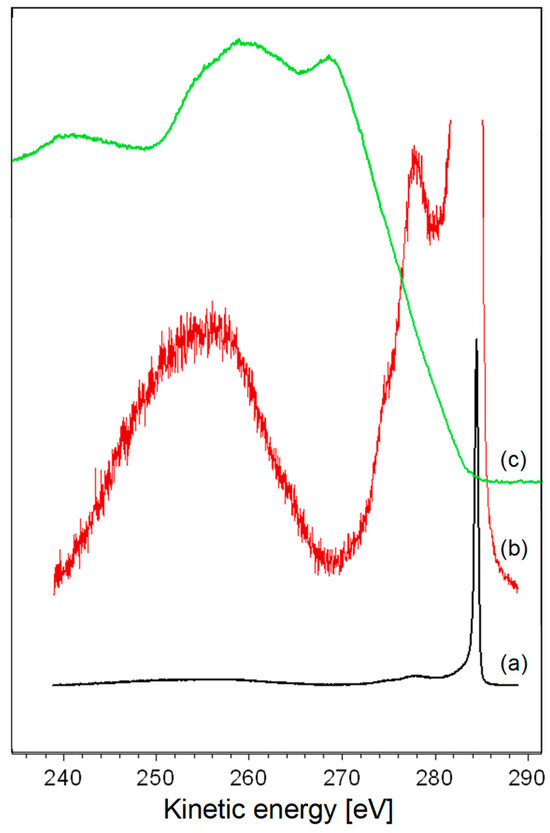
Figure 1.
(a) Position of the core and loss features aligned on the kinetic energy scale of the Auger spectrum; (b) amplified view of the C 1s loss feature; and (c) Auger spectrum.
Another consideration regards the convolution process. If m is the number of elements of f and n is the number of elements of g, by definition, the convolution h is composed of m + n elements. However, by considering Equations (11) or (12), the value of f n+1 (i.e., a function composed by n elements) is obtained through a calculation that involves a convolution (n + m elements). However, when we examine Equations (11) or (12), we find that the calculation for obtaining the value of f n+1 (a function composed of n elements) involves a convolution with n + m elements. As previously mentioned, this issue can be addressed by multiplying the vector h and the matrix G with its transpose GT and applying Equations (11) or (12) when the relaxation factor μ is utilized. It is worth noting that attempts to use GTh as a reference to model the Auger spectrum in the van Cittert iterations have proven unsuccessful. The modeled function f n has failed to accurately describe the original Auger spectrum. This suggests that GTh may not be a suitable reference for reproducing the Auger spectrum through van Cittert iterations. In RxpsG, the deconvolution option utilizes either the FFT or the van Cittert algorithm. Attempting to deconvolve the loss feature associated with the high-energy tail of the core lines from the corresponding Auger spectrum using FFT results in outcomes marked by unacceptable levels of noise, as anticipated. Conversely, the alternative van Cittert algorithm necessitates a procedure to reduce the sum of m + n points to m, as outlined in Equation (10). The flowchart of the deconvolution routine is shown in Figure 2.
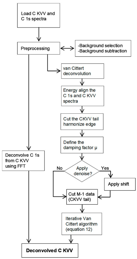
Figure 2.
Flowchart of the deconvolution routine. For clarity, the scheme refers to CKVV and C 1s spectra.
In addressing this challenge, RxpsG retains m data corresponding to the convolution’s portion with a higher spectral power, while the remaining n − 1 points describing the featureless tail at a low kinetic energy are disregarded. This approach leverages a specific property of the convolution function. Given a generic function f with m elements and the Dirac function δ with n elements, it follows that
f ⨂ g = fc
Here, fc is equal to f plus n additional zeros introduced by the convolution with the delta function. In our case, the C 1s core line exhibits sharpness resembling a δ function, with the peak situated near the high-kinetic-energy edge. Consequently, the convolution of the Auger and the C 1s yields a spectrum consisting of a portion closely resembling the original Auger spectrum in the highly kinetic region and a featureless tail in the remaining low-energy region. This can be easily verified by checking the FWHM of C KVV ⨂ C 1s, which appears to be almost the same as that of the original C KVV spectrum. Then, C KVV ⨂ C 1s accumulates the information in a region with an extension substantially equal to that of the original Auger spectrum. This enables the selection of a spectral portion comprising m data points by aligning them with the original spectrum to minimize errors. The additional n points forming the tail can be neglected, as illustrated in Figure 3.
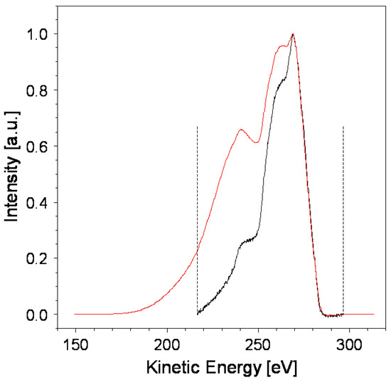
Figure 3.
Original background-subtracted Auger spectrum (black) and the C KVV ⨂ C 1s convolution (red). The dashed line indicates the point where the convolution will be truncated. The dashed lines delimit the portion of the spectrum used for the deconvolution. In particular, at a low kinetic energy the featureless tail is disregarded during the van Cittert iteration process.
In Figure 3, truncating the featureless tail of the convolved spectrum introduces a discontinuity point because, at low kinetic energies, the edge is non-zero. The FFT transform of a transition to a non-null value in zero-time, such as in the case of a δ function or a square wave, contains all frequencies. For similar reasons, when computing the convolution using the van Cittert algorithm, it is evident that the discontinuity at the edge leads to spectral distortions.
In RxpsG, this issue is addressed by applying a damping factor to align the edges of the original and convolved spectra, as illustrated in Figure 4a,b. This damping factor serves to mitigate the spectral distortions arising from the discontinuity at the edge, ensuring a more accurate representation of the convolved spectrum without introducing artifacts.
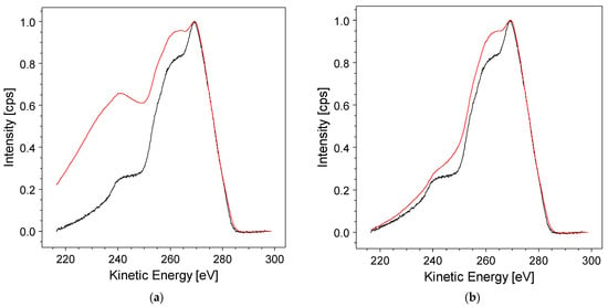
Figure 4.
Applying a damping factor to harmonize the low-kinetic-energy (KE) tail of the convolved spectrum from the van Cittert algorithm (in red) with the original background-subtracted Auger spectrum (in black). Panels show results for different damping factors: (a) damping factor = 0.1; and (b) damping factor = 0.8.
Now, the iterative van Cittert algorithm can be applied. The signal-to-noise ratio (SNR) of the original spectra (Auger and C 1s in this example) may vary under different acquisition conditions. So, simple minimization of the standard deviation is insufficient to determine when to stop the iteration. Due to the low number of cycles required for convergence, the RxpsG software prompts users at each step to decide whether another iteration is needed to achieve a better result. Figure 5 illustrates the situation at the beginning and after the six iteration cycles sufficient to reproduce the original CKVV spectrum (black) using the convolution of the modeled CKVV with the C 1s (red spectrum). The green trace representing the spectral difference between the modeled and original spectra is approximately zero in the whole energy range.
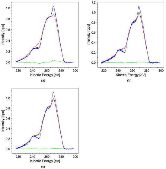
Figure 5.
The result of the Van Cittert iteration at the beginning, with the original data (black), G′ f n convolution (red) iteration = 1 in (a), iteration = 6 in (b,c), the deconvolved spectrum (blue), and the difference h′ − G′ f n (green); (b) after six iterations, the convolution overlaps the original data, and the difference is almost null in the whole energy range; (c) when the Denoise option is selected, a less noisy deconvolved spectrum (blue) is obtained.
Upon observing the deconvolved spectrum (depicted in blue), it becomes evident that the iterative process contributes to a rise in spectral noise. To address this issue, the software provides a Denoise option, aiming to control the level of noise in the deconvolved spectrum. Opting for this feature involves applying a slight shift either forward and backward of μ [h′ − G′ f n] with respect to f n (refer to Equation (13)) during each iteration. This procedure leads to noise reduction, resulting in an improved and acceptable spectrum.
Figure 5b,c display the deconvolution outcomes obtained without and with the application of the Denoise procedure, respectively. As is discernible, there is a noticeable reduction in the superimposed noise on the deconvolved spectrum (depicted in blue) in the second case, occurring just after six iterations. This option proves to be particularly effective, especially in scenarios where a higher number of cycles is necessary for convergence, leading to a substantial decrease in the noise level.
5. Algorithm Testing
The results of the proposed method were tested to assess the van Cittert algorithm’s ability to accurately deconvolve loss features from the Auger CKVV spectrum. The objective was to evaluate the outcome when applying the inverse operation to reproduce the original spectrum. To achieve this, we started with Equation (18), providing the deconvolved spectrum f n+1. In our example, f n+1 represents the deconvolved Auger spectrum at iteration n + 1. If f n+1 correctly describes the deconvolved CKVV spectrum, then f n+1 ⨂ g, where g is the C 1s core line, must replicate the original Auger data. We compared f n+1 ⨂ g with the CKVV spectrum for different iteration numbers. The results are illustrated in Figure 6.
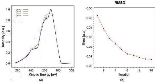
Figure 6.
(a) Comparison of the original Auger CKVV spectrum with the convolution result f n+1 ⨂ g, f n+1 representing the output of the van Cittert method and g the C 1s spectrum, at iterations three, six, and nine; (b) root mean square difference (RMSD) between the original Auger spectrum and the convolution result f n+1 ⨂ g as a function of the iteration number.
As evident from Figure 6a, increasing the number of iterations enhances the fidelity of reproducing the original spectrum. This trend is further illustrated in Figure 6b, where the root mean square deviation (RMSD) between the original Auger spectrum and the result obtained from the f n+1 ⨂ g convolution is plotted against the number of iterations. The RMSD decreases with each iteration, although the improvement in reproduction fidelity tends to plateau after the sixth iteration.
6. Conclusions
In conclusion, this discussion has focused on the deconvolution of loss features from the Auger spectra of carbon. Drawing from the past and present literature, guidance is provided for the correct pre-processing of the original data, specifically emphasizing accurate background subtraction and energy alignment of the spectra. The deconvolved spectrum is obtained by applying the van Cittert algorithm. However, the direct application of the iterative procedure requires caution due to the mismatch of the number of elements between convolution and the original spectrum in the van Cittert algorithm. Reproduction tests have confirmed that RxpsG provides a reliable method for accurately calculating the deconvolved spectrum. This involves selecting the appropriate data segment and utilizing a denoising option to effectively minimize noise in the resultant spectrum.
Funding
This research received no external funding.
Institutional Review Board Statement
No ethical approval is required for this research.
Informed Consent Statement
The study did not involve humans.
Data Availability Statement
Data are available on request using the corresponding author e-mail address.
Conflicts of Interest
The author declares no conflicts of interest.
References
- Pantin, E.; Starck, J.-L.; Murtagh, F. Deconvolution and Blind Deconvolution in Astronomy. In Blind Image Deconvolution. Theory and Applications, 1st ed.; CRC Press: Boca Raton, FL, USA, 2007. [Google Scholar]
- San, O.; Vedula, P. Generalized Deconvolution Procedure for Structural Modeling of Turbulence. J. Sci. Comput. 2018, 75, 1187–1206. [Google Scholar] [CrossRef]
- Grediac, M.; Blaysat, B.; Sur, F. A Robust-to-Noise Deconvolution Algorithm to Enhance Displacement and Strain Maps Obtained with Local DIC and LSA. Exp. Mech. 2018, 59, 219–243. [Google Scholar] [CrossRef]
- Flores-Llamas, H. Marriage of the Burger-Van Cittert and Allen deconvolution methods yields a highly improved overlapping line resolver. Rev. Sci. Instrum. 1995, 66, 3989–3993. [Google Scholar] [CrossRef]
- Cantoni, V.; De Lotto, I.; Ghirardi, A. DEO, A program to deconvolve experimental outcomes. Nucl. Instr. Methods 1978, 153, 199–205. [Google Scholar] [CrossRef]
- Law, J.; Hogan, D. Profile deconvolution. Nucl. Instr. Methods Phys. Res. B 1984, 5, 67–74. [Google Scholar] [CrossRef]
- Vesely, V. FFT-based processing of unresolved spectra with multiple convolutions. Nucl. Instr. Methods Phys. Res. B 1986, 18, 88–100. [Google Scholar] [CrossRef]
- Briggs, D.; Seah, M.P. Practical Surface Analysis by Auger and Photoelecron Spectroscopies; J. Wiley & Sons: Chichester, UK, 1990. [Google Scholar]
- Briggs, D.; Grant, J.T. Surface Analysis by Auger and X-ray Photoelectron Spectroscopies, 1st ed.; IM Publications and Surface Spectra: Trowbridge, UK, 2003. [Google Scholar]
- Briggs, D. Surface Analysis of Polymers by XPS and Static SIMS; Cambridge University Press: Cambridge, UK, 1998. [Google Scholar]
- Speranza, G. Data Driven Guide to the Analysis of X-ray Photoelectron Spectra Using RxpsG, 1st ed.; CRC-Francis and Taylor: Boca Raton, FL, USA, 2023. [Google Scholar]
- Rye, R.R.; Houston, J.E. Molecular Auger spectroscopy. Acc. Chem. Res. 1984, 17, 41–47. [Google Scholar] [CrossRef]
- Agren, H.; Cesar, A.; Liegener, C.M. Theory of Molecular Auger Spectra. Adv. Quant. Chem. 1992, 23, 1–82. [Google Scholar]
- Gel’mukhanov, F.; Agren, H.; Svensson, S.; Aksela, H.; Aksela, S. Theory of Auger spectra for molecular-field-split core levels. Phys. Rev. A 1996, 53, 1379–1387. [Google Scholar] [CrossRef]
- Smith, M.A.; Levenson, L.L. Valence-band information from the Auger K VV spectrum of graphite. Phys. Rev. B 1977, 16, 2973–2977. [Google Scholar] [CrossRef]
- Murday, J.S.; Dunlap, B.I.; Huston, F.L.; Oelhafen, P. Carbon KVV Auger line shapes of graphite and stage-one cesium and lithium intercalated graphite. Phys. Rev. B 1981, 24, 4764–4770. [Google Scholar] [CrossRef]
- Dunlap, B.I.; Ramaker, D.E.; Murday, J.S. Effect of screening on the carbon KVV Auger line shape of alkali-metal — intercalated graphite. Phys. Rev. B 1982, 25, 6439–6446. [Google Scholar] [CrossRef]
- Jennison, D.R. Initial-State Relaxation Effects in Molecular Auger Spectra. Phys. Rev. A 1981, 23, 1215–1222. [Google Scholar] [CrossRef]
- Mularie, W.M.; Peria, W.T. Deconvolution techniques in Auger Spectroscopy. Surf. Sci. 1971, 26, 125–141. [Google Scholar] [CrossRef]
- Houston, J.E.; Rogers, J.W.; Rye, R.R.; Huston, F.L.; Ramaker, D.D. Relationship between the Auger line shape and the electronic properties of graphite. Phys. Rev. B 1986, 34, 1215–1226. [Google Scholar] [CrossRef]
- Bandzuch, P.; Morhac, M.; Kristiak, T. Study of the Van Cittert and Gold iterative methods of deconvolution and their application in the deconvolution of experimental spectra of positron annihilation. Nucl. Instr. Methods Phys. Res. A 1997, 384, 506–515. [Google Scholar] [CrossRef]
- Golla, S.S.V.; Lubberink, M.; van Berckel, B.N.M.; Lammertsma, A.A.; Boellaard, R. Partial volume correction of brain PET studies using iterative deconvolution in combination with HYPR denoising. EJNMMI Res. 2017, 7, 36. [Google Scholar] [CrossRef]
- Bergmann, T.G.; Schluter, N. Introducing Alternative Algorithms for the Determination of the Distribution of Relaxation Times. ChemPhysChem 2022, 23, e202200012. [Google Scholar] [CrossRef] [PubMed]
- Xu, C.; Assaoui, I.; Jacquery, S. Algebraic analysis of the van Cittert iterative method of deconvolution with a general relaxation factor. J. Opt. Soc. Am. A 1994, 11, 2084. [Google Scholar] [CrossRef]
- Morhac, M.; Matousek, V.; Kliman, J. Optimized multidimensional nonoscillating deconvolution. J. Comp. Appl. Math. 2002, 140, 639–658. [Google Scholar] [CrossRef][Green Version]
- Mazzieri, G.L.; Spies, R.D. Regularization methods for ill-posed problems in multiple Hilbert scales. Inverse Probl. 2012, 28, 055005. [Google Scholar] [CrossRef]
- Tychonoff, A.N.; Arsenin, V.Y. Solution of Ill-Posed Problems; Winston & Sons: Washington, DC, USA, 1977. [Google Scholar]
- Riley, J.D. Solving systems of linear equations with a positive definite, symmetric, but possibly ill-conditioned matrix. Math. Tables Aids Comput. 1956, 9, 96–101. [Google Scholar]
- Richardson, W. Bayesian-based iterative method of image restoration. J. Opt. Soc. Am. 1972, 62, 55–59. [Google Scholar] [CrossRef]
- Lucy, L. An iterative technique for the rectification of observed distributions. Astron. J. 1974, 79, 745. [Google Scholar] [CrossRef]
- Van Cittert, P.H. Zum Einfluß der Spaltbreite auf die Intensitätsverteilung in Spektrallinien. II. Z. Physik. 1931, 69, 298–303. [Google Scholar] [CrossRef]
- Von Burger, H.C.; can Cittert, P.H. Wahre und scheinbare Intensitätsverteilung in Spektrallinien. Z. Physik. 1932, 69, 722–730. [Google Scholar] [CrossRef]
- Hill, N.R.; Ioup, G.E. Convergence of the van Cittert iterative method of deconvolution. J. Opt. Soc. Am. 1976, 66, 487–489. [Google Scholar] [CrossRef]
- Jansson, P.A. Method for determining the response function of a high resolution infrared spectrometer. J. Opt. Soc. Am. 1970, 60, 184–191. [Google Scholar] [CrossRef]
- Speranza, G.; Canteri, R. RxpsG a new open project for Photoelectron and Electron Spectroscopy data processing. SoftwareX 2019, 10, 100282. [Google Scholar] [CrossRef]
- Tougaard, S. Practical algorithm for background subtraction. Surf. Sci. 1989, 216, 343–360. [Google Scholar] [CrossRef]
Disclaimer/Publisher’s Note: The statements, opinions and data contained in all publications are solely those of the individual author(s) and contributor(s) and not of MDPI and/or the editor(s). MDPI and/or the editor(s) disclaim responsibility for any injury to people or property resulting from any ideas, methods, instructions or products referred to in the content. |
© 2024 by the author. Licensee MDPI, Basel, Switzerland. This article is an open access article distributed under the terms and conditions of the Creative Commons Attribution (CC BY) license (https://creativecommons.org/licenses/by/4.0/).