

A Robust Recurrent Neural Networks-Based Surrogate Model for Thermal History and Melt Pool Characteristics in Directed Energy Deposition

 , ,
, ,  ,
, 
Abstract
1. Introduction
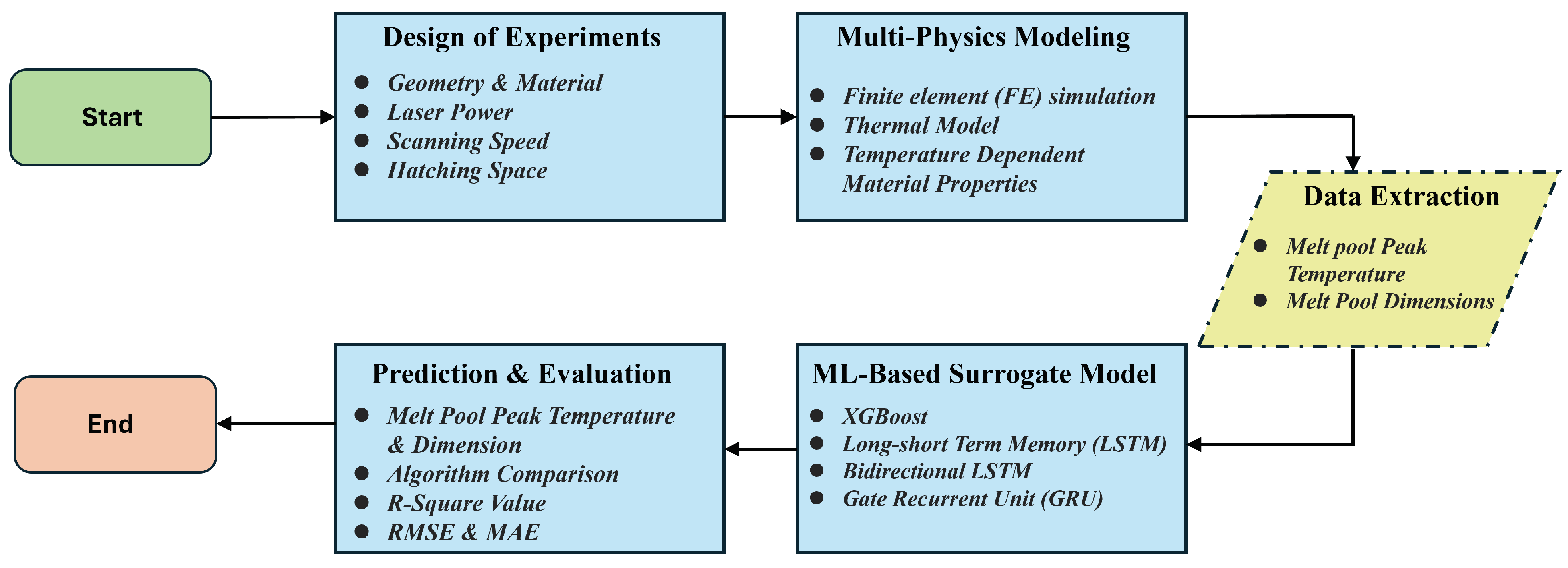
2. Methodology
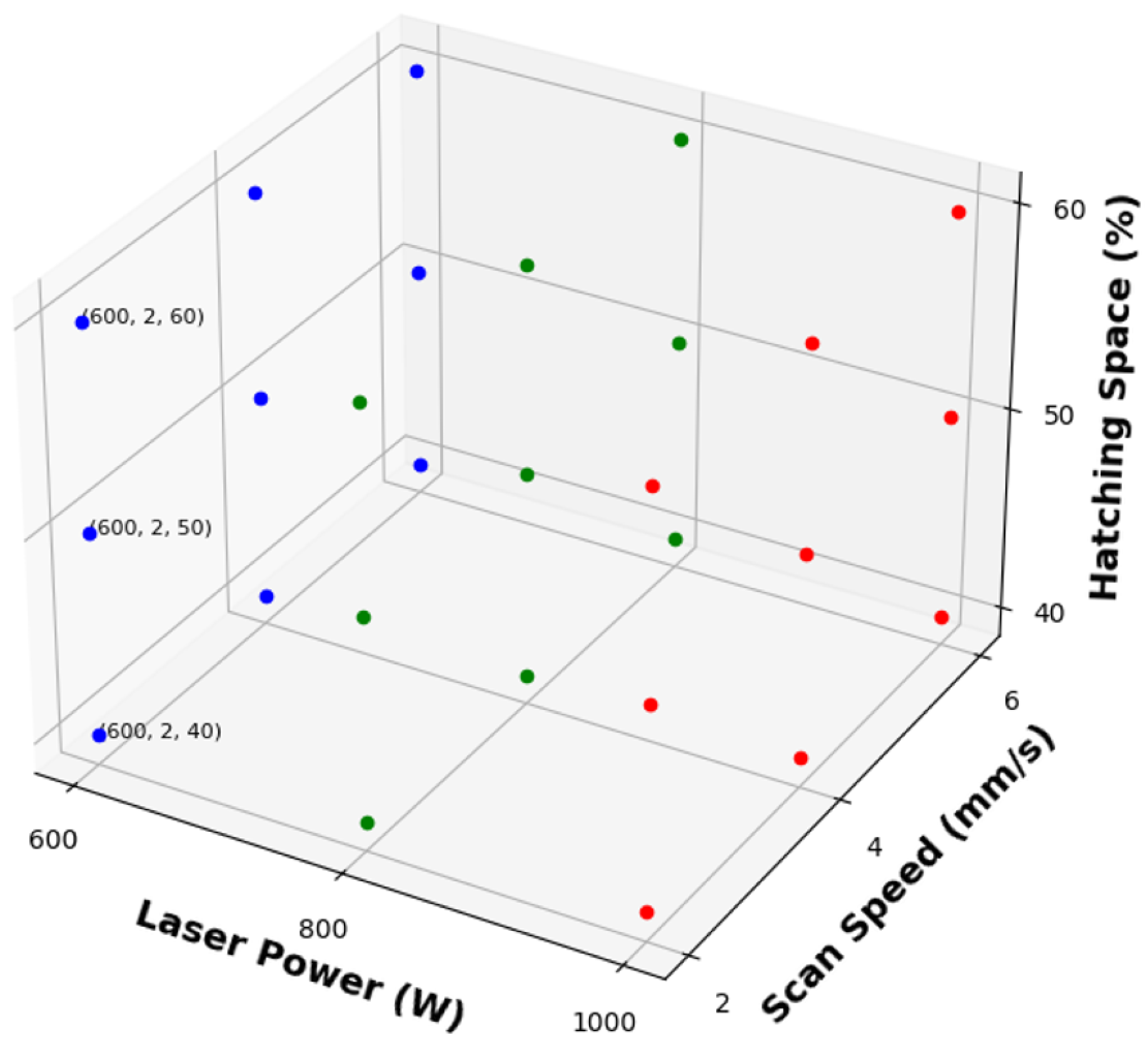
2.1. Design of Experiments
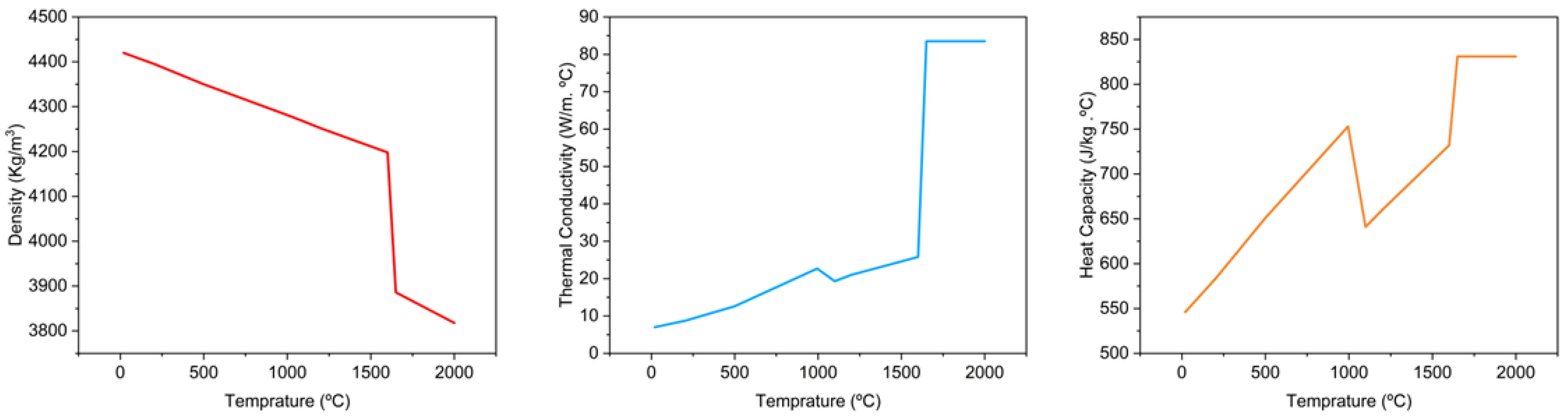
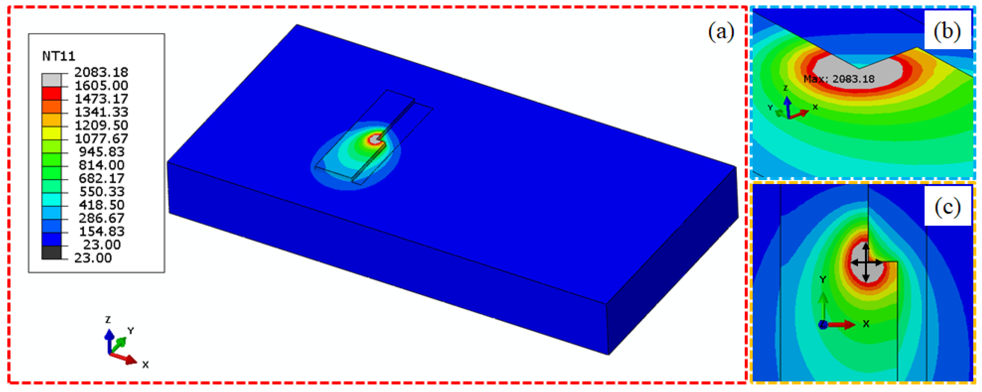
2.2. Multi-Physics Simulation
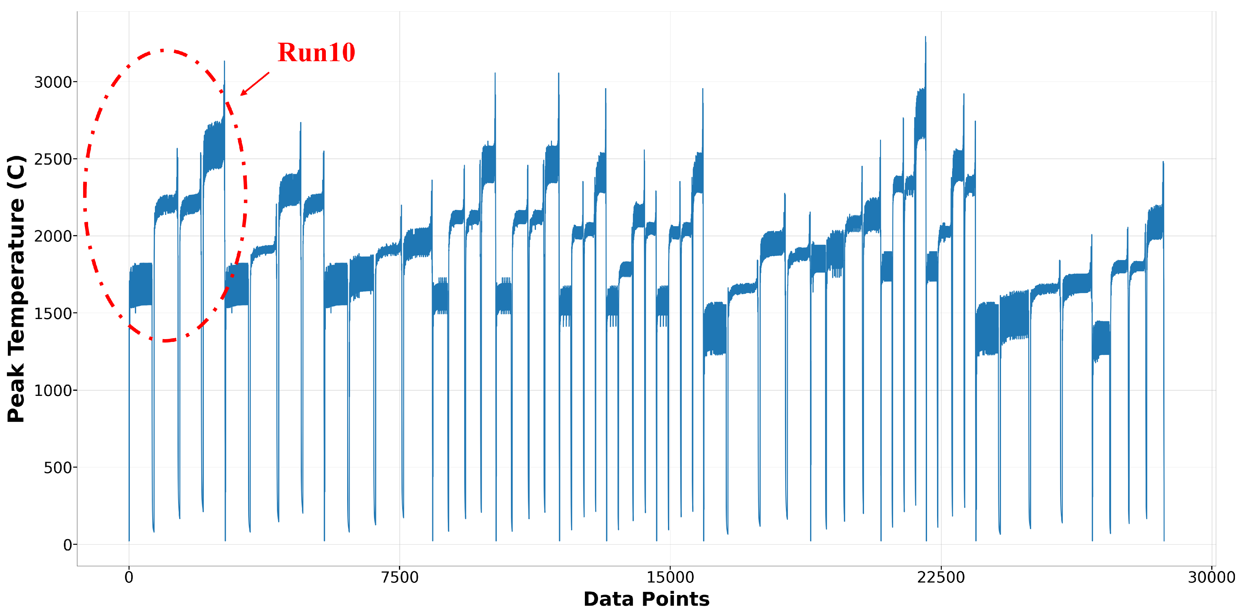
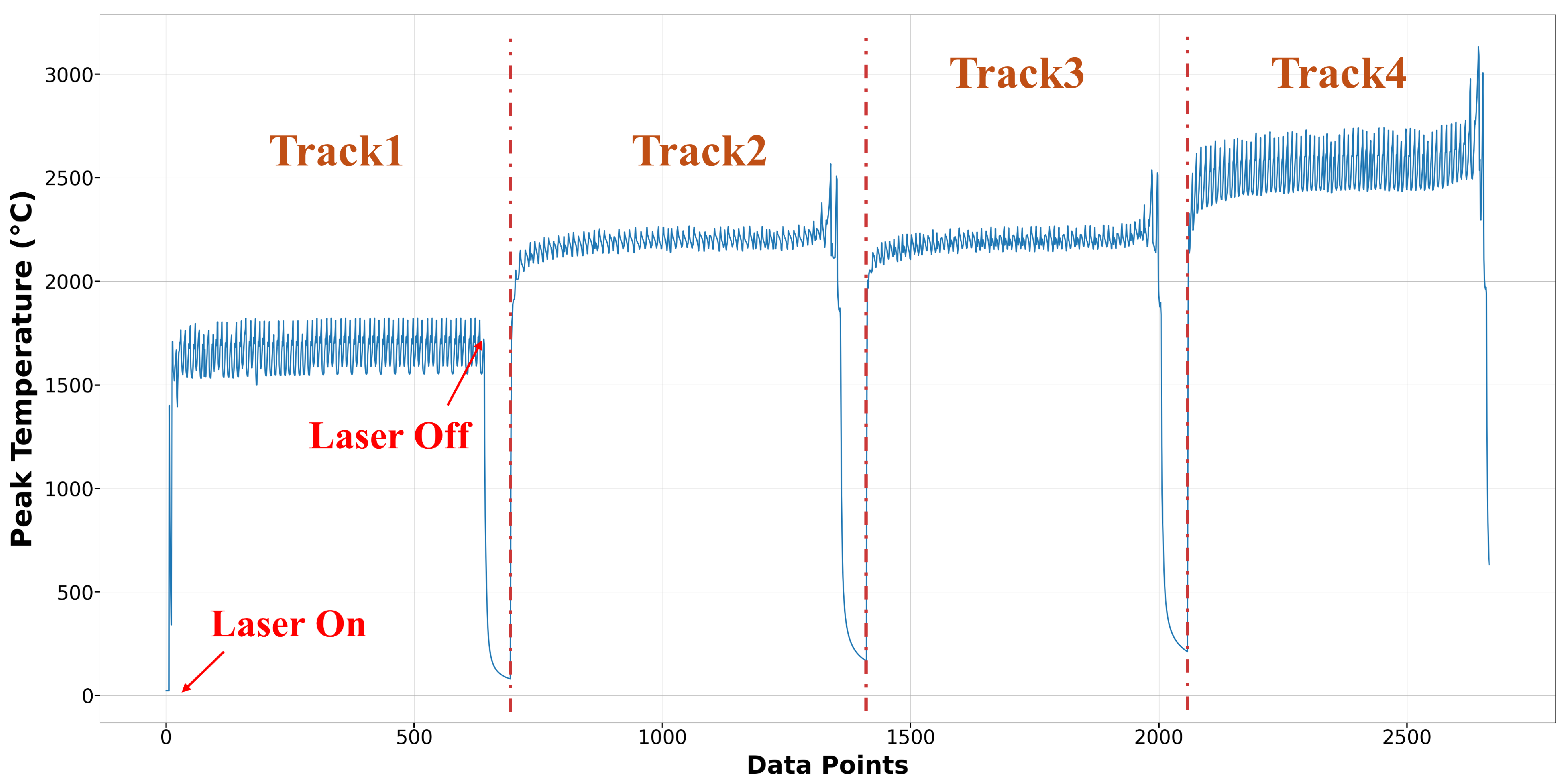
2.3. Data Generation and Extraction
2.4. Machine Learning Models
2.4.1. Extreme Gradient Boosting (XGBoost)
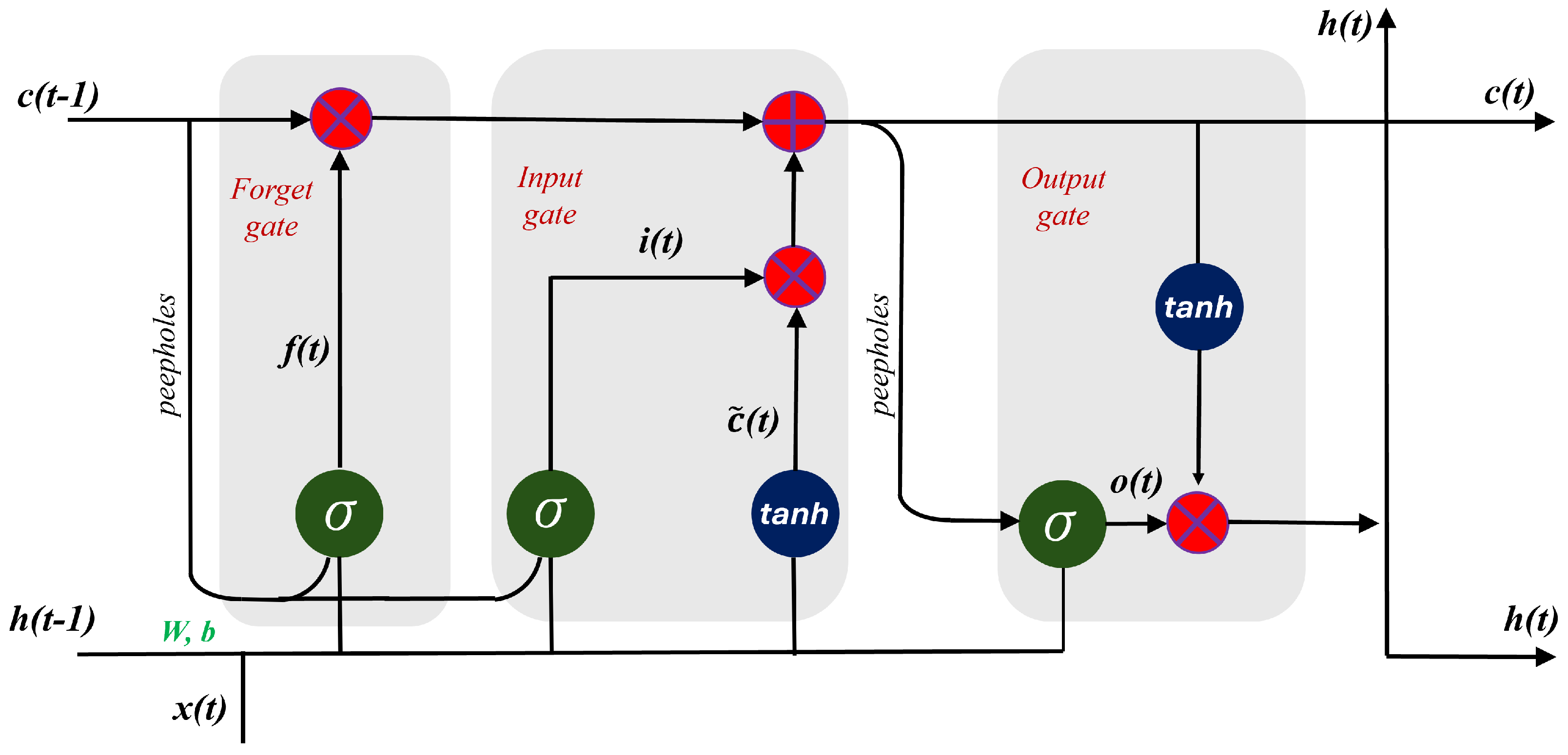
2.4.2. Long Short-Term Memory (LSTM)
2.4.3. Bidirectional Long Short-Term Memory (Bi-LSTM)
2.4.4. Gated Recurrent Units (GRUs)
2.4.5. Model Evaluation
3. Results and Discussion
3.1. Data Pre-Processing and Model Training
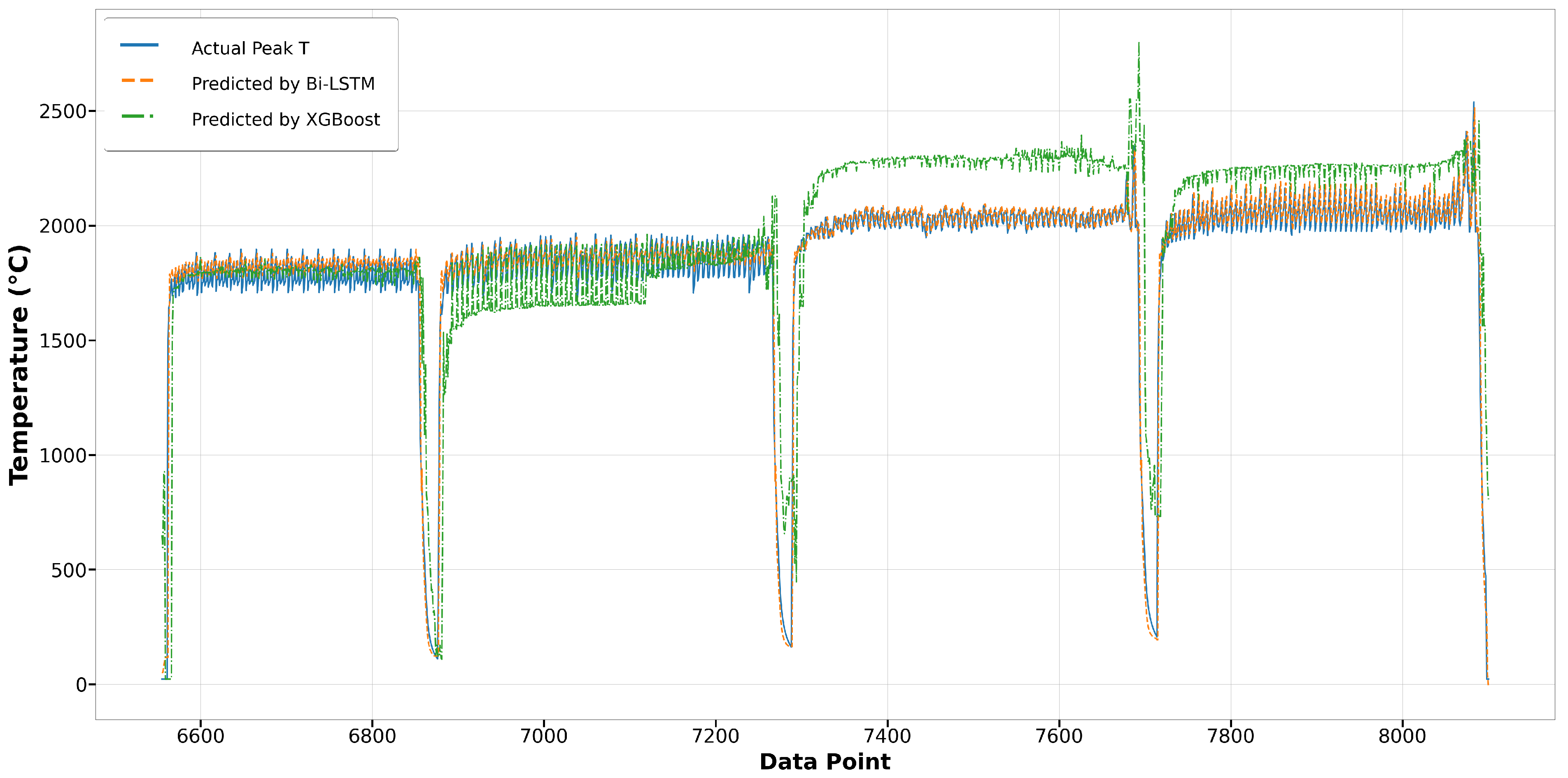
3.2. Melt Pool Peak Temperature Model
3.3. Melt Pool Geometry Model
3.3.1. Melt Pool Length Model
3.3.2. Melt Pool Width Model
3.3.3. Melt Pool Depth Model
4. Conclusions
- Robust Model Architecture: Employed advanced RNN architectures—LSTM, Bi-LSTM, and GRU—to effectively capture the sequential and dynamic behavior of melt pools in DED processes.
- High Predictive Accuracy: Achieved an R-square of 0.983 for melt pool peak temperature predictions using the Bi-LSTM algorithm. Demonstrated superior performance in melt pool geometry predictions:
- -
- Melt pool length: R-square of 0.903 with the GRU algorithm.
- -
- Melt pool width: R-square of 0.952 with the Bi-LSTM algorithm.
- -
- Melt pool depth: R-square of 0.885 with the GRU algorithm.
- Efficiency and Robustness: The GRU-based surrogate model outperformed other algorithms in terms of accuracy, computation time, and memory usage, showing a reduction of at least 29% in computation time and 50% in memory usage, highlighting the model’s efficiency and robustness.
Author Contributions
Funding
Data Availability Statement
Conflicts of Interest
References
- Svetlizky, D.; Das, M.; Zheng, B.; Vyatskikh, A.L.; Bose, S.; Bandyopadhyay, A.; Schoenung, J.M.; Lavernia, E.J.; Eliaz, N. Directed energy deposition (DED) additive manufacturing: Physical characteristics, defects, challenges and applications. Mater. Today 2021, 49, 271–295. [Google Scholar] [CrossRef]
- Xie, J.; Zhou, Y.; Zhou, C.; Li, X.; Chen, Y. Microstructure and mechanical properties of Mg–Li alloys fabricated by wire arc additive manufacturing. J. Mater. Res. Technol. 2024, 29, 3487–3493. [Google Scholar] [CrossRef]
- Madhavadas, V.; Srivastava, D.; Chadha, U.; Raj, S.A.; Sultan, M.T.H.; Shahar, F.S.; Shah, A.U.M. A review on metal additive manufacturing for intricately shaped aerospace components. CIRP J. Manuf. Sci. Technol. 2022, 39, 18–36. [Google Scholar] [CrossRef]
- Saboori, A.; Aversa, A.; Marchese, G.; Biamino, S.; Lombardi, M.; Fino, P. Application of directed energy deposition-based additive manufacturing in repair. Appl. Sci. 2019, 9, 3316. [Google Scholar] [CrossRef]
- Tariq, U.; Wu, S.H.; Mahmood, M.A.; Woodworth, M.M.; Liou, F. Effect of pre-heating on residual stresses and deformation in laser-based directed energy deposition repair: A comparative analysis. Materials 2024, 17, 2179. [Google Scholar] [CrossRef]
- Mohd Yusuf, S.; Cutler, S.; Gao, N. The impact of metal additive manufacturing on the aerospace industry. Metals 2019, 9, 1286. [Google Scholar] [CrossRef]
- Piscopo, G.; Iuliano, L. Current research and industrial application of laser powder directed energy deposition. Int. J. Adv. Manuf. Technol. 2022, 119, 6893–6917. [Google Scholar] [CrossRef]
- Markets, R. Market Opportunities for Directed Energy Deposition Manufacturing. Available online: https://www.researchandmarkets.com/reports/4850372/market-opportunities-for-directed-energy (accessed on 6 June 2024).
- Brennan, M.; Keist, J.; Palmer, T. Defects in metal additive manufacturing processes. J. Mater. Eng. Perform. 2021, 30, 4808–4818. [Google Scholar] [CrossRef]
- Yuhua, C.; Yuqing, M.; Weiwei, L.; Peng, H. Investigation of welding crack in micro laser welded NiTiNb shape memory alloy and Ti6Al4V alloy dissimilar metals joints. Opt. Laser Technol. 2017, 91, 197–202. [Google Scholar] [CrossRef]
- Chen, Y.; Sun, S.; Zhang, T.; Zhou, X.; Li, S. Effects of post-weld heat treatment on the microstructure and mechanical properties of laser-welded NiTi/304SS joint with Ni filler. Mater. Sci. Eng. A 2020, 771, 138545. [Google Scholar] [CrossRef]
- Ertay, D.S.; Naiel, M.A.; Vlasea, M.; Fieguth, P. Process performance evaluation and classification via in-situ melt pool monitoring in directed energy deposition. CIRP J. Manuf. Sci. Technol. 2021, 35, 298–314. [Google Scholar] [CrossRef]
- Jiang, H.Z.; Li, Z.Y.; Feng, T.; Wu, P.Y.; Chen, Q.S.; Feng, Y.L.; Chen, L.F.; Hou, J.Y.; Xu, H.J. Effect of process parameters on defects, melt pool shape, microstructure, and tensile behavior of 316L stainless steel produced by selective laser melting. Acta Metall. Sin. (English Lett.) 2021, 34, 495–510. [Google Scholar] [CrossRef]
- Liu, M.; Kumar, A.; Bukkapatnam, S.; Kuttolamadom, M. A review of the anomalies in directed energy deposition (DED) processes & potential solutions-part quality & defects. Procedia Manuf. 2021, 53, 507–518. [Google Scholar]
- Zheng, B.; Haley, J.; Yang, N.; Yee, J.; Terrassa, K.; Zhou, Y.; Lavernia, E.; Schoenung, J. On the evolution of microstructure and defect control in 316L SS components fabricated via directed energy deposition. Mater. Sci. Eng. A 2019, 764, 138243. [Google Scholar] [CrossRef]
- Xie, J.; Chen, Y.; Wang, H.; Zhang, T.; Zheng, M.; Wang, S.; Yin, L.; Shen, J.; Oliveira, J. Phase transformation mechanisms of NiTi shape memory alloy during electromagnetic pulse welding of Al/NiTi dissimilar joints. Mater. Sci. Eng. A 2024, 893, 146119. [Google Scholar] [CrossRef]
- Mahmood, M.A.; Popescu, A.C.; Oane, M.; Channa, A.; Mihai, S.; Ristoscu, C.; Mihailescu, I.N. Bridging the analytical and artificial neural network models for keyhole formation with experimental verification in laser melting deposition: A novel approach. Results Phys. 2021, 26, 104440. [Google Scholar] [CrossRef]
- Wu, Y.; Wu, H.; Zhao, Y.; Jiang, G.; Shi, J.; Guo, C.; Liu, P.; Jin, Z. Metastable structures with composition fluctuation in cuprate superconducting films grown by transient liquid-phase assisted ultra-fast heteroepitaxy. Mater. Today Nano 2023, 24, 100429. [Google Scholar] [CrossRef]
- Wu, S.H.; Joy, R.; Tariq, U.; Mahmood, M.A.; Liou, F. Role of In-Situ Monitoring Technique for Digital Twin Development Using Direct Energy Deposition: Melt Pool Dynamics and Thermal Distribution; University of Texas at Austin: Austin, TX, USA, 2023. [Google Scholar]
- Yeoh, Y. Decoupling Part Geometry from Microstructure in Directed Energy Deposition Technology: Towards Reliable 3D Printing of Metallic Components. Ph.D. Thesis, Nanyang Technological University, Singapore, 2021. [Google Scholar]
- Kistler, N.A.; Corbin, D.J.; Nassar, A.R.; Reutzel, E.W.; Beese, A.M. Effect of processing conditions on the microstructure, porosity, and mechanical properties of Ti-6Al-4V repair fabricated by directed energy deposition. J. Mater. Process. Technol. 2019, 264, 172–181. [Google Scholar] [CrossRef]
- Tariq, U.; Joy, R.; Wu, S.H.; Arif Mahmood, M.; Woodworth, M.M.; Liou, F. Optimization of Computational Time for Digital Twin Database in Directed Energy Deposition for Residual Stresses; University of Texas at Austin: Austin, TX, USA, 2023. [Google Scholar]
- Hooper, P.A. Melt pool temperature and cooling rates in laser powder bed fusion. Addit. Manuf. 2018, 22, 548–559. [Google Scholar] [CrossRef]
- He, W.; Shi, W.; Li, J.; Xie, H. In-situ monitoring and deformation characterization by optical techniques; part I: Laser-aided direct metal deposition for additive manufacturing. Opt. Lasers Eng. 2019, 122, 74–88. [Google Scholar] [CrossRef]
- Nuñez, L., III; Sabharwall, P.; van Rooyen, I.J. In situ embedment of type K sheathed thermocouples with directed energy deposition. Int. J. Adv. Manuf. Technol. 2023, 127, 3611–3623. [Google Scholar] [CrossRef]
- Zhao, M.; Wei, H.; Mao, Y.; Zhang, C.; Liu, T.; Liao, W. Predictions of Additive Manufacturing Process Parameters and Molten Pool Dimensions with a Physics-Informed Deep Learning Model. Engineering 2023, 23, 181–195. [Google Scholar] [CrossRef]
- Wang, Z.; Wang, C.; Zhang, S.; Qiu, L.; Lin, Y.; Tan, J.; Sun, C. Towards high-accuracy axial springback: Mesh-based simulation of metal tube bending via geometry/process-integrated graph neural networks. Expert Syst. Appl. 2024, 255, 124577. [Google Scholar] [CrossRef]
- De Borst, R. Challenges in computational materials science: Multiple scales, multi-physics and evolving discontinuities. Comput. Mater. Sci. 2008, 43, 1–15. [Google Scholar] [CrossRef]
- Darabi, R.; Azinpour, E.; Reis, A.; de Sa, J.C. Multi-scale multi-physics phase-field coupled thermo-mechanical approach for modeling of powder bed fusion process. Appl. Math. Model. 2023, 122, 572–597. [Google Scholar] [CrossRef]
- Zhao, T.; Yan, Z.; Zhang, B.; Zhang, P.; Pan, R.; Yuan, T.; Xiao, J.; Jiang, F.; Wei, H.; Lin, S.; et al. A comprehensive review of process planning and trajectory optimization in arc-based directed energy deposition. J. Manuf. Process. 2024, 119, 235–254. [Google Scholar] [CrossRef]
- Bayat, M.; Dong, W.; Thorborg, J.; To, A.C.; Hattel, J.H. A review of multi-scale and multi-physics simulations of metal additive manufacturing processes with focus on modeling strategies. Addit. Manuf. 2021, 47, 102278. [Google Scholar] [CrossRef]
- Zhu, Q.; Liu, Z.; Yan, J. Machine learning for metal additive manufacturing: Predicting temperature and melt pool fluid dynamics using physics-informed neural networks. Comput. Mech. 2021, 67, 619–635. [Google Scholar] [CrossRef]
- Qi, X.; Chen, G.; Li, Y.; Cheng, X.; Li, C. Applying neural-network-based machine learning to additive manufacturing: Current applications, challenges, and future perspectives. Engineering 2019, 5, 721–729. [Google Scholar] [CrossRef]
- Akbari, P.; Ogoke, F.; Kao, N.Y.; Meidani, K.; Yeh, C.Y.; Lee, W.; Farimani, A.B. MeltpoolNet: Melt pool characteristic prediction in Metal Additive Manufacturing using machine learning. Addit. Manuf. 2022, 55, 102817. [Google Scholar] [CrossRef]
- Zhu, X.; Jiang, F.; Guo, C.; Wang, Z.; Dong, T.; Li, H. Prediction of melt pool shape in additive manufacturing based on machine learning methods. Opt. Laser Technol. 2023, 159, 108964. [Google Scholar] [CrossRef]
- Zhang, Z.; Liu, Z.; Wu, D. Prediction of melt pool temperature in directed energy deposition using machine learning. Addit. Manuf. 2021, 37, 101692. [Google Scholar] [CrossRef]
- Jones, K.; Yang, Z.; Yeung, H.; Witherell, P.; Lu, Y. Hybrid modeling of melt pool geometry in additive manufacturing using neural networks. In Proceedings of the International Design Engineering Technical Conferences and Computers and Information in Engineering Conference; American Society of Mechanical Engineers: New York, NY, USA, 2021; Volume 85376, p. V002T02A031. [Google Scholar]
- Mahmood, M.A.; Ishfaq, K.; Khraisheh, M. Inconel-718 processing windows by directed energy deposition: A framework combining computational fluid dynamics and machine learning models with experimental validation. Int. J. Adv. Manuf. Technol. 2024, 130, 3997–4011. [Google Scholar] [CrossRef]
- Tariq, U.; Joy, R.; Wu, S.H.; Mahmood, M.A.; Malik, A.W.; Liou, F. A state-of-the-art digital factory integrating digital twin for laser additive and subtractive manufacturing processes. Rapid Prototyp. J. 2023, 29, 2061–2097. [Google Scholar] [CrossRef]
- Lu, X.; Lin, X.; Chiumenti, M.; Cervera, M.; Hu, Y.; Ji, X.; Ma, L.; Yang, H.; Huang, W. Residual stress and distortion of rectangular and S-shaped Ti-6Al-4V parts by Directed Energy Deposition: Modelling and experimental calibration. Addit. Manuf. 2019, 26, 166–179. [Google Scholar] [CrossRef]
- Newkirk, J. Multi-Layer Laser Metal Deposition Process. Ph.D. Thesis, Missouri University of Science and Technology Rolla, Rolla, MO, USA, 2014. [Google Scholar]
- Wu, S.H.; Tariq, U.; Joy, R.; Sparks, T.; Flood, A.; Liou, F. Experimental, computational, and machine learning methods for prediction of residual stresses in laser additive manufacturing: A critical review. Materials 2024, 17, 1498. [Google Scholar] [CrossRef]
- Gouge, M.; Michaleris, P.; Denlinger, E.; Irwin, J. The finite element method for the thermo-mechanical modeling of additive manufacturing processes. In Thermo-Mechanical Modeling of Additive Manufacturing; Elsevier: Amsterdam, The Netherlands, 2018; pp. 19–38. [Google Scholar]
- Dhieb, N.; Ghazzai, H.; Besbes, H.; Massoud, Y. Extreme gradient boosting machine learning algorithm for safe auto insurance operations. In Proceedings of the 2019 IEEE International Conference on Vehicular Electronics and Safety (ICVES), Cairo, Egypt, 4–6 September 2019; pp. 1–5. [Google Scholar]
- Yu, Y.; Si, X.; Hu, C.; Zhang, J. A review of recurrent neural networks: LSTM cells and network architectures. Neural Comput. 2019, 31, 1235–1270. [Google Scholar] [CrossRef]


| Process Parameters (Unit) | Values |
|---|---|
| Laser Power (W) | 600, 800, 1000 |
| Scanning Speed (mm/s) | 2, 4, 6 |
| Hatching Space (%) | 40, 50, 60 |
| Laser Beam Size (mm) | 2 |
| Layer Thickness (mm) | 0.5 |
| Thermal Properties | Shown in Figure 4 |
| Run | Laser Power (W) | Scanning Speed (mm/s) | Hatch Space (%) |
|---|---|---|---|
| 1 | 600 | 2 | 60 |
| 2 | 600 | 2 | 50 |
| 3 | 600 | 2 | 40 |
| 4 | 600 | 4 | 60 |
| 5 | 600 | 4 | 50 |
| 6 | 600 | 4 | 40 |
| 7 | 600 | 6 | 60 |
| 8 | 600 | 6 | 50 |
| 9 | 600 | 6 | 40 |
| 10 | 800 | 2 | 60 |
| 11 | 800 | 2 | 50 |
| 12 | 800 | 2 | 40 |
| 13 | 800 | 4 | 60 |
| 14 | 800 | 4 | 50 |
| 15 | 800 | 4 | 40 |
| 16 | 800 | 6 | 60 |
| 17 | 800 | 6 | 50 |
| 18 | 800 | 6 | 40 |
| 19 | 1000 | 2 | 60 |
| 20 | 1000 | 2 | 50 |
| 21 | 1000 | 2 | 40 |
| 22 | 1000 | 4 | 60 |
| 23 | 1000 | 4 | 50 |
| 24 | 1000 | 4 | 40 |
| 25 | 1000 | 6 | 60 |
| 26 | 1000 | 6 | 50 |
| 27 | 1000 | 6 | 40 |
| Model | Training Data | Testing Data | Training Size | Testing Size | Features | Labels |
|---|---|---|---|---|---|---|
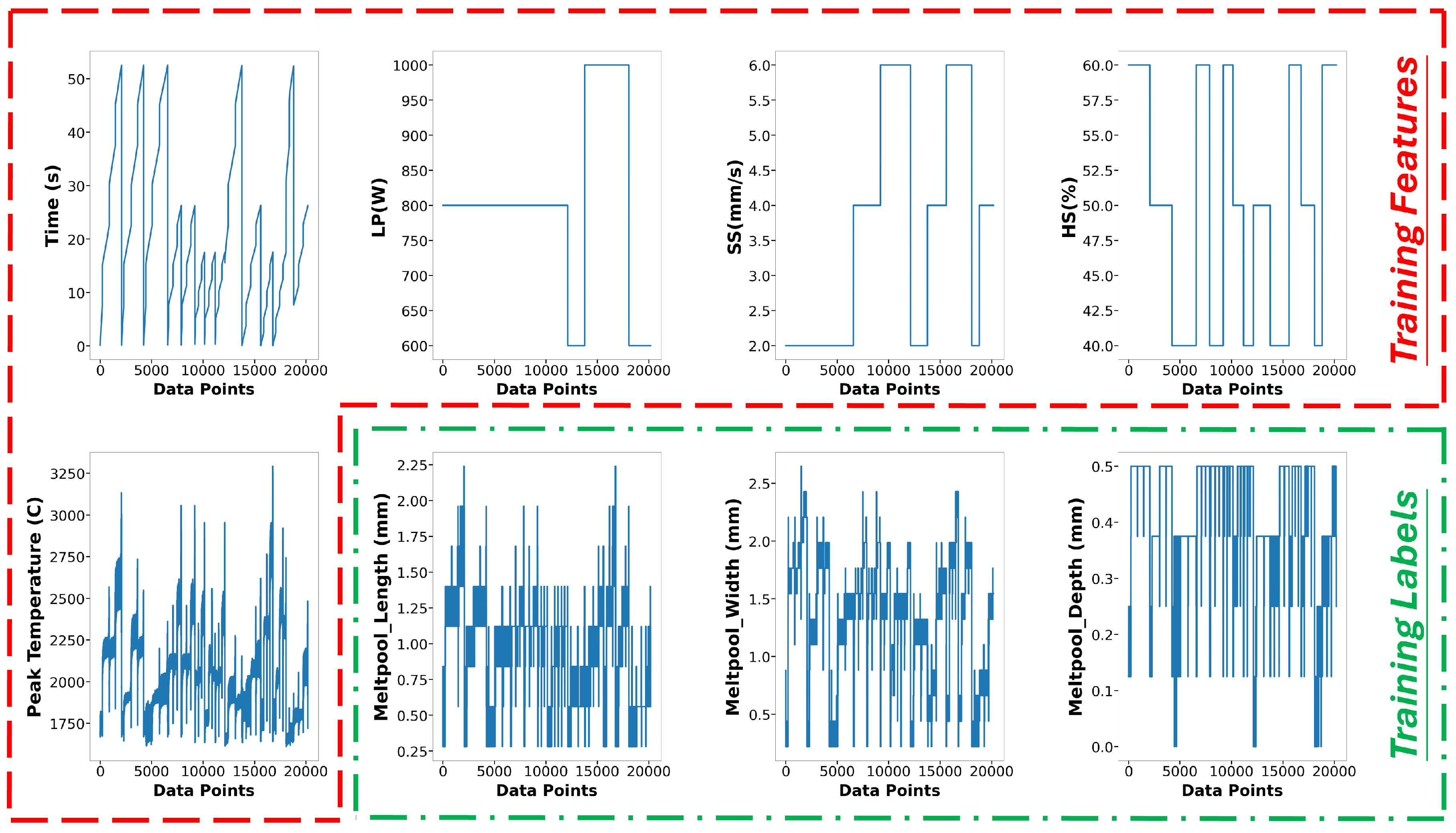
| Melt Pool Peak Temperature | Run2-4, Run10-13, Run15-18, Run24-26 | Run1, Run5, Run14, Run23, Run27 | 28,683 | 10,184 | Time, Position X, Y, Z, Laser Power, Scanning Speed, Hatch Space | Melt Pool Peak Temperature |
| Melt Pool Dimension | Run2-4, Run10-13, Run15-18, Run24-26 | Run1, Run5, Run14, Run23, Run27 | 20,182 | 7590 | Time, Peak Temperature, Laser Power, Scanning Speed, Hatch Space | Melt Pool Length, Melt Pool Width, Melt Pool Depth |
| Algorithms | R-Square | RMSE | MAE | Computation Time (s) | Memory Usage (GB) |
|---|---|---|---|---|---|
| XGBoost | 0.852 | 0.0550 | 0.0382 | 16.67 | 0.747 |
| LSTM | 0.979 | 0.0178 | 0.0126 | 238.60 | 2.41 |
| Bi-LSTM | 0.983 | 0.0153 | 0.0101 | 290.25 | 5.24 |
| GRU | 0.978 | 0.0179 | 0.0129 | 189.30 | 2.28 |
| Algorithms | R-Square | RMSE | MAE | Computation Time (s) | Memory Usage (GB) |
|---|---|---|---|---|---|
| XGBoost | 0.698 | 0.1031 | 0.0629 | 16.22 | 0.269 |
| LSTM | 0.888 | 0.0539 | 0.0412 | 76.23 | 1.37 |
| Bi-LSTM | 0.902 | 0.0501 | 0.0369 | 120.55 | 2.65 |
| GRU | 0.903 | 0.0503 | 0.0381 | 67.75 | 1.30 |
| Algorithms | R-Square | RMSE | MAE | Computation Time (s) | Memory Usage (GB) |
|---|---|---|---|---|---|
| XGBoost | 0.752 | 0.0963 | 0.0762 | 16.95 | 0.371 |
| LSTM | 0.946 | 0.0418 | 0.0313 | 86.26 | 1.37 |
| Bi-LSTM | 0.952 | 0.0399 | 0.0293 | 128.70 | 2.65 |
| GRU | 0.951 | 0.04 | 0.0291 | 76.73 | 1.30 |
| Algorithms | R-Square | RMSE | MAE | Computation Time (s) | Memory Usage (GB) |
|---|---|---|---|---|---|
| XGBoost | 0.751 | 0.0892 | 0.0555 | 20.20 | 0.344 |
| LSTM | 0.871 | 0.0479 | 0.0360 | 97.69 | 1.44 |
| Bi-LSTM | 0.881 | 0.0476 | 0.0359 | 120.19 | 2.72 |
| GRU | 0.885 | 0.0420 | 0.0293 | 85.43 | 1.37 |
Disclaimer/Publisher’s Note: The statements, opinions and data contained in all publications are solely those of the individual author(s) and contributor(s) and not of MDPI and/or the editor(s). MDPI and/or the editor(s) disclaim responsibility for any injury to people or property resulting from any ideas, methods, instructions or products referred to in the content. |
© 2024 by the authors. Licensee MDPI, Basel, Switzerland. This article is an open access article distributed under the terms and conditions of the Creative Commons Attribution (CC BY) license (https://creativecommons.org/licenses/by/4.0/).
Share and Cite
Wu, S.-H.; Tariq, U.; Joy, R.; Mahmood, M.A.; Malik, A.W.; Liou, F. A Robust Recurrent Neural Networks-Based Surrogate Model for Thermal History and Melt Pool Characteristics in Directed Energy Deposition. Materials 2024, 17, 4363. https://doi.org/10.3390/ma17174363
Wu S-H, Tariq U, Joy R, Mahmood MA, Malik AW, Liou F. A Robust Recurrent Neural Networks-Based Surrogate Model for Thermal History and Melt Pool Characteristics in Directed Energy Deposition. Materials. 2024; 17(17):4363. https://doi.org/10.3390/ma17174363
Chicago/Turabian StyleWu, Sung-Heng, Usman Tariq, Ranjit Joy, Muhammad Arif Mahmood, Asad Waqar Malik, and Frank Liou. 2024. "A Robust Recurrent Neural Networks-Based Surrogate Model for Thermal History and Melt Pool Characteristics in Directed Energy Deposition" Materials 17, no. 17: 4363. https://doi.org/10.3390/ma17174363
APA StyleWu, S.-H., Tariq, U., Joy, R., Mahmood, M. A., Malik, A. W., & Liou, F. (2024). A Robust Recurrent Neural Networks-Based Surrogate Model for Thermal History and Melt Pool Characteristics in Directed Energy Deposition. Materials, 17(17), 4363. https://doi.org/10.3390/ma17174363