Abstract
In this work, we present a quantitative method for determining the concentration of metal oxide nanoparticles (NP) synthesized by laser ablation in liquid. The case study was performed with titanium dioxide nanoparticles (TiO2 NP), which were synthesized by laser ablation of a Ti target in water. After synthesis, a colloidal solution was analyzed with UV-Vis spectroscopy. At the same time, the craters that remained on the Ti target after ablation were evaluated with an optical microscope to determine the volume of the ablated material. SEM microscopy was used to determine the TiO2 NP size distribution. It was found that synthesized TiO2 NP followed a Log-Normal diameter distribution with a maximum at about 64 nm. From the volume of ablated material and NP size distribution, under the assumption that most of the ablated material is consumed to form nanoparticles, a concentration of nanoparticles can be determined. The proposed method is verified by comparing the calculated concentrations to the values obtained from the Beer–Lambert law using the Mie scattering theory for the NP cross-section calculation.
1. Introduction
Pulsed laser ablation in liquid (PLAL) is a versatile method for the synthesis of colloidal solutions of nanoparticles (NP) [1]. In this method, the laser pulses hit the target immersed in liquid and cause a laser-induced breakdown, followed by the shock wave and plasma plume formation, its expansion and cooling, cavitation bubble formation, and its expansion and collapse [2]. Nanoparticles are produced during the plasma cooling phase in the processes of nucleation and condensation. After the collapse of the cavitation bubble, nanoparticles are released and diffused into the liquid, leading to the formation of a colloidal solution of NP [2]. Because of the liquid environment, the plasma plume is very strongly confined and therefore has a much larger temperature, pressure, and density compared to the ablation in gas [3]. Unlike ablation in gas, there is no need for a closed chamber for NP collection in PLAL. The liquid layer around the plasma plume is also transformed into the plasma phase, leading to a mixture of two plasmas so chemical reactions can take place between them, thus affecting the NP structure [3]. For instance, the ablation of a Ti target in deionized water with a NS laser at a wavelength of 1064 nm results in the synthesis of TiO2 NP, as in the present work [4].
A PLAL-synthesized colloidal solution of NP usually has large stability due to the presence of a negative charge on the NP surface [5]. The main advantages of PLAL over chemical methods of NP fabrication are the high purity of synthesized nanoparticles, the absence of unwanted residual byproducts in NP colloidal solution, and the possibility of NP synthesis from a large variety of materials [6]. The properties of NP properties, such as morphology, size distribution, and crystal structure, are affected by PLAL parameters such as laser fluence, wavelength, ablation spot size, pulse duration, type of liquid, and presence of surfactants in it. Therefore, there is a large space for modification and engineering of NP properties [7].
The concentration of nanoparticles in colloidal solution is a very important parameter for their application, for example, in biomedical applications [8,9], cancer treatment [10], detectors [11], solar cells, drug delivery, energy storage [12] and photocatalysis [13]. Furthermore, information about NP concentration is important for assessing reproducibility, compliance with regulation, and risk evaluation [14]. Many methods are developed for direct counting or indirect calculation of NP concentration in a colloidal solution. Some of the experimental techniques used for this purpose are [15]: dynamic light scattering (DLS) [16,17], turbidimetry [18,19], optical particle counter [20], NP tracking analysis [17,21,22], single-particle inductively coupled plasma mass spectroscopy (spICPMS) [23], UV-Vis spectroscopy [24,25], resistive-pulse sensing [26], and magnetic NP imaging (MPI) [9].
Most of these methods have serious limitations in achieving accurate determinations of NP concentration. For example, the size limitation of NP (in turbidimetry, resistive pulse-sensing, NP tracking analysis), overshadowing the signal of the small nanoparticles (in DLS), or the need for having calibration solution (in DLS and spICMS) [15]. An additional consideration for these methods is the difficulty in sampling, whereby diluting the as-prepared sample over several orders of magnitude is often needed. The main disadvantage of determining concentration from UV-Vis is the need for knowledge of the NP size and refractive indices.
In our previous work [27], a simple model for calculating PLAL-synthesized pure metallic NP concentrations is introduced that considers the volume of an ablated crater and NP size distribution. All disadvantages existing in the previously mentioned methods for concentration calculation do not exist here. The only limitations are those related to the accuracy of crater volume and size distribution determination. This model is successfully tested for Ag NP synthesized by laser ablation of Ag target using Beer–Lambert law.
In the present work, we show that this model can be adapted for the calculation of the concentration of metal oxide NP synthesized by PLAL of the metallic targets that are very prone to oxidation. The proposed method is tested for TiO2 NP synthesized by the laser ablation of a Ti target immersed in water. TiO2 NP have stability, corrosion resistance, low reactivity, long agglomeration, and sedimentation time. They have a broad range of industrial and scientific applications, especially photocatalysis [28]. The well-known phases of TiO2 are anatase, rutile, and brookite, while amorphous TiO2, as one synthesized in this work, is much less investigated. Although amorphous TiO2 is characterized by lower photocatalytic performance than one of the crystal phases, it can act as an active component for visible and near-IR light-harvesting, leading to improved photocatalytic activity in this part of the light energy spectrum, so it can also be applied in photodegradation of organic dyes, hydrogen production, and CO2 photoreduction [29].
Furthermore, amorphous TiO2 has lower toxicity and better corrosion resistance when compared to TiO2 in the crystal phase, which can be an advantage in photoprotective and cosmetic applications [30]. It also exhibits excellent antibacterial properties [31], while a special energy band structure and improved charge separation may be advantageous in SERS [29]. Amorphous TiO2 NP can be easily transformed to a crystalline phase by heat treatment [29], thus retaining the NP concentration value.
To verify this method, concentrations of TiO2 NP calculated from crater volume (CV) were compared to the concentrations obtained from the UV-Vis photoabsorbance data using Beer–Lambert law and Mie scattering theory (CA). Beer–Lambert law is usually used for the calculation of the concentration of metal nanoparticles with a well-defined resonant frequency, for example, gold [24,32,33] or silver as in [27]. In the case of TiO2, such calculation is more complicated because it is not plasmonic material. Still, it is a semiconductor that absorbs mainly in the UV range, so it does not possess resonant frequency. Furthermore, TiO2 refractive index at some wavelength depends on many parameters such as TiO2 bandgap, crystal structure, defects in it, and NP size [34,35], thus it is not easy to ensure that correct values of refraction index from literature are taken for calculation of CA. Moreover, the dipole approximation that was satisfied in [27] due to the sufficiently small size of synthesized Ag nanoparticles (<λSPR/10, where λSPR ≈ 400 nm is silver absorption peak) is not applicable in the present work dealing with NP, which are much larger and do not possess resonant frequency. Thus, in the present paper, model verification by the Beer–Lambert law is adapted when compared to the same method used in [27] to be applicable for the determination of semiconductor NP concentration, and the Mie theory for the calculation of TiO2 NP extinction cross-section is exactly applied instead of using the dipole approximation.
2. Materials and Methods
A colloidal solution of TiO2 NP was synthesized by the pulsed-laser ablation of the Ti target (purity 99.9% and thickness 3 mm, Kurt J. Lesker) immersed in a beaker containing 40 mL of deionized water using Nd:YAG laser (Quantell, Brilliant). Laser specifications are a pulse duration of 4 ns, wavelength of 1064 nm, output energy of 290 mJ and repetition rate of 5 Hz. The laser beam was directed by a system of prisms and focused by a lens (the focal length of 10 cm) onto the target surface. The laser pulse energy in front of the target was 210 mJ while a diameter of a focused pulse on the target surface was 1 mm, which yielded a laser fluence of 27 J/cm2. The thickness of a water layer above the target was kept constant at 2 cm during the experiment to keep the ablation efficiency and thus the NP properties, constant [36]. The target was fixed during the experiments to allow the drilling of a crater and thus determine ablated material mass. A scheme of the experimental setup for PLAL is depicted in detail in [37].
After the experiments, the craters created on the targets were studied with an optical microscope (Leica DM2700M, Leica Microsystems, Wetzlar, Germany). Microscopical images were taken at different focal positions with respect to the target surface in order to obtain crater radius dependence on crater depth (i.e., crater profile). Using the obtained crater profile, crater volume is calculated according to the procedure described in [38].
The optical absorbance of laser synthesized colloidal solutions was assessed using a UV-Vis spectrophotometer (Lambda 25, Perkin Elmer, Waltham, MA, USA) in the wavelength range of 200–600 nm.
The crystallinity and crystalline phases were studied by grazing incidence X-ray diffraction (GIXRD). To perform a structural characterization of TiO2 NP, the produced colloid was dropped onto a silicon substrate and left to air-dry to obtain TiO2 NP film. The crystalline structure of TiO2 NP was investigated using a D5000 diffractometer (Siemens, Munich, Germany) in a parallel beam geometry with Cu Kα radiation, a point detector, and a collimator in front of the detector. Grazing incidence X-ray diffraction (GIXRD) scans were acquired with the constant incidence angle αi of 1°, ensuring that the information contained in the collected signal covers the entire film thickness.
The morphology and size distribution of the synthesized nanoparticles was studied by a field emission scanning electron microscope (FE-SEM, JSM-7600F, Jeol Ltd., Tokyo, Japan). Samples for SEM imaging were prepared by depositing one drop of a suspension on a polished Al sample holder. The holder with the specimens was coated with a 3 nm-thick amorphous carbon layer (PECS 682) prior to the SEM imaging. SEM images were analyzed with ImageJ to determine the NP size distribution.
A Zetasizer Ultra (Malvern Panalytical, Malvern, UK) was used to determine the zeta-potential (ζ) by electrophoretic light scattering (ELS). It was calculated from the measured electrophoretic mobility by means of the Henry equation using the Smoluchowski approximation (f(ka) = 1.5). Results are reported as an average value of three measurements. The data processing was done by the ZS Xplorer 1.20 (Malvern Panalytical).
Numerical calculations of extinction, scattering, and absorption cross-sections of TiO2 NP using equations from Mie scattering theory are performed by Mätzler’s MATLAB code [39].
3. Results
3.1. TiO2 NP Characterization
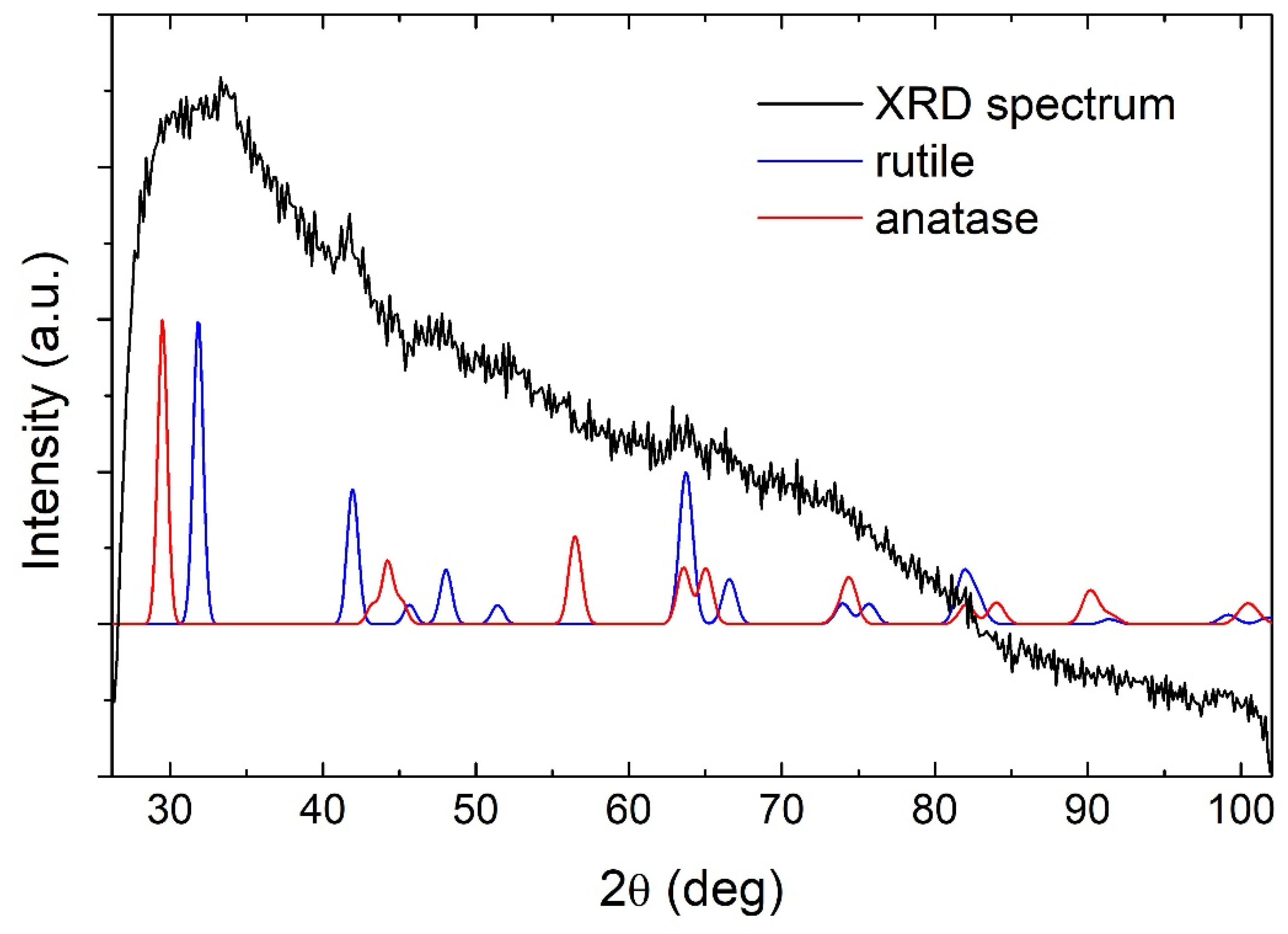
The laser ablation of metallic Ti target in water resulted in the synthesis of a colloidal solution of semiconductor TiO2 NP. The GIXRD measurements shown in Figure 1 revealed that TiO2 NP are amorphous due to the lack of appearance of any of the major Bragg peaks of TiO2 phases (theoretical peaks for rutile and anatase are shown for comparison). The ζ-potential of the produced TiO2 NP colloidal solution was measured to be 30 ± 1 mV, making the solution of moderate stability (aggregation and precipitation of nanoparticles appeared after two days). Therefore, TiO2 NP concentration can also be considered a homogenous and well-defined value in the as-prepared solution.

Figure 1.
GIXRD pattern of TiO2 nanoparticles.
The morphology and size distribution of TiO2 NP were obtained using SEM imaging. A typical SEM image of TiO2 NP is shown in Figure 2a, where 5000 pulses were applied in ablation. It can be seen that TiO2 NP are spherical and with a broad range of sizes. For each number of laser pulses applied in ablation, the size distribution was obtained by measuring the diameters of 200 single nanoparticles from SEM images. It was found that the size distribution was similar for all tested numbers of pulses. The size distribution obtained from SEM images is shown in Figure 2b.
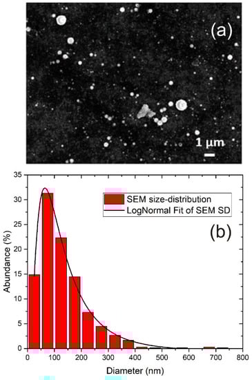
Figure 2.
(a) SEM image of TiO2 nanoparticles (5000 pulses applied in ablation) and (b) size distribution of TiO2 NP from SEM including Log-Normal Fit.
It can be seen that the size distribution is relatively broad, and it was fitted with the Log-Normal function with the maximum at 64 nm. Log-Normal is a very common function for fitting the size distribution of nanoparticles synthesized by PLAL [40,41,42,43]. Although non-NP species are, to some degree, also present in synthesized colloidal solutions, such as large debris structures, from the obtained size distribution in Figure 2b, it can be assumed that their presence is negligible, so the term “TiO2 NP” is justified. Since the nanoparticles are spherical, the average NP volume is calculated as , where d is nanoparticle diameter and can be obtained from the size distribution. From the given size distribution in Figure 2b, the average volume of nanoparticles is calculated as:
where M is the total number of size ranges in the size distribution, di is the average diameter that corresponds to size range i (single column bar in size distribution), and ni = Ni/N is the ratio between the number Ni of nanoparticles corresponding to size range i (relative abundance of NP within corresponding column bar) and the total number of nanoparticles N. Equation (1) gives = 3.45 × 10⁻³ μm3.
3.2. Calculation of TiO2 NP Concentration from Crater Volume (CV)
The mass of synthesized TiO2 NP depends on the amount of ablated material by PLAL, represented as a volume of a crater left on the target after ablation. Due to the fact that the target was made of almost pure titanium (thickness of surface oxidation layer can be neglected when compared to crater volume), the amount of titanium in the formed TiO2 NP is coming solely from the target while the oxygen is coming from the water. The volume of the ablated crater Vcrat is turned into a fraction of titanium in the synthesized TiO2 NP. The total number N of synthesized nanoparticles can be determined from the known volume of ablated material Vcrat by performing the following calculation:
where N is the total number of nanoparticles in colloidal solution, is the average volume of nanoparticles, m(TiO2) is the total mass of TiO2 NP in colloidal solution, ρ(Ti) is Ti target density (4.506 g/cm3 near R.T.), ρ(TiO2) is the TiO2 NP density (3.8 ± 0.1 g/cm3) for amorphous TiO2 [44], while m(Ti) and m(O2) are the total masses of titanium and oxygen atoms in TiO2 NP in colloidal solution, respectively. A(O) and A(Ti) are atomic mass numbers for oxygen atom and titanium atom, which are 16 and 48, respectively. As shown in [45], TiO2 NP of 21 nm in size have only 4% larger density than TiO2 particles 200 nm in size, so it can be concluded that, due to the prevalence of large nanoparticles in the TiO2 NP size distribution (Figure 2b), it is justified to neglect the NP size dependence of ρ(TiO2) in Equation (2).
Number concentration CV [mL−1] of TiO2 nanoparticles is then Equation (3):
where total number of synthesized nanoparticles is divided by an amount of liquid Vliquid where synthesis was performed (in our case Vliquid = 40 mL).
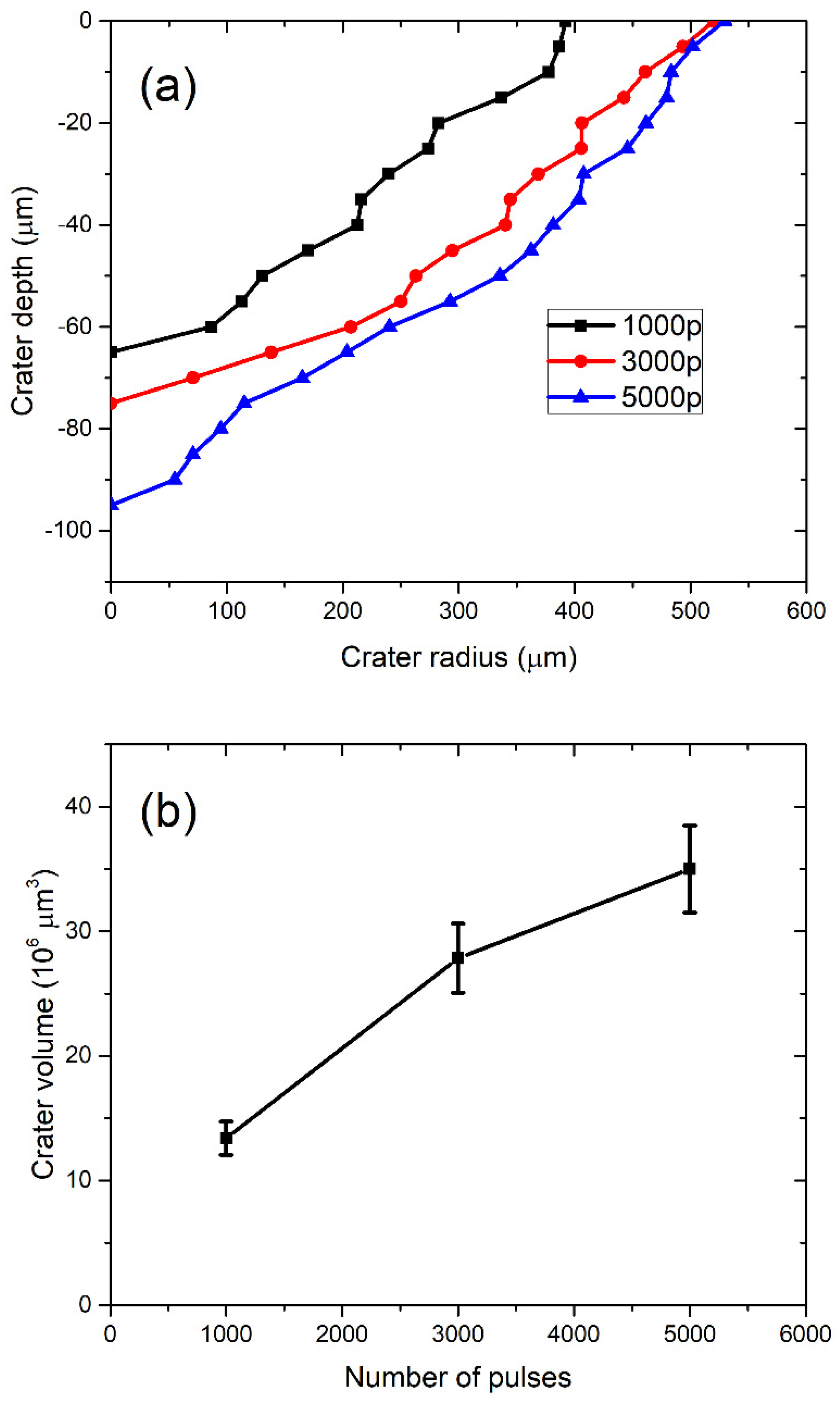
In Figure 3a, the profiles of craters left after ablation with 1000, 3000, and 5000 applied laser pulses are shown (note that the x–y axis is not in scale). The dashed line denotes the target surface. Craters are characterized by a relatively large aspect ratio (radius to depth), as the depth of a crater is about five times lower than the crater radius. In Figure 3b, the volumes of crater Vcrat dependent on the number of pulses are shown, where volumes are calculated from profiles in Figure 3a, as described in [38]. For each number of applied pulses, the total number of nanoparticles in water is calculated by inserting the measured Vcrat in Equation (2). It provides the following number of nanoparticles dependence on number of pulses: N (1000p) = 7.69 × 10⁹, N (3000p) = 15.94 × 10⁹, N (5000p) = 20.04 × 10⁹. When the number of nanoparticles N is divided by water volume Vliquid = 40 mL, as in Equation (3), the concentration CV of TiO2 NP is obtained for each number of applied pulses. Their values are CV (1000p) = (1.9 ± 0.2) × 108 mL−1, CV (3000p) = (4.0 ± 0.4) × 108 mL−1 and CV (5000p) = (5.0 ± 0.5) × 108 mL−1.
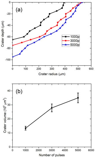
Figure 3.
(a) Profiles of craters remained on the Ti target after ablation and (b) ablation crater volume dependence on the number of pulses.
3.3. Calculation of TiO2 NP Concentration from Beer–Lambert Law (CA)
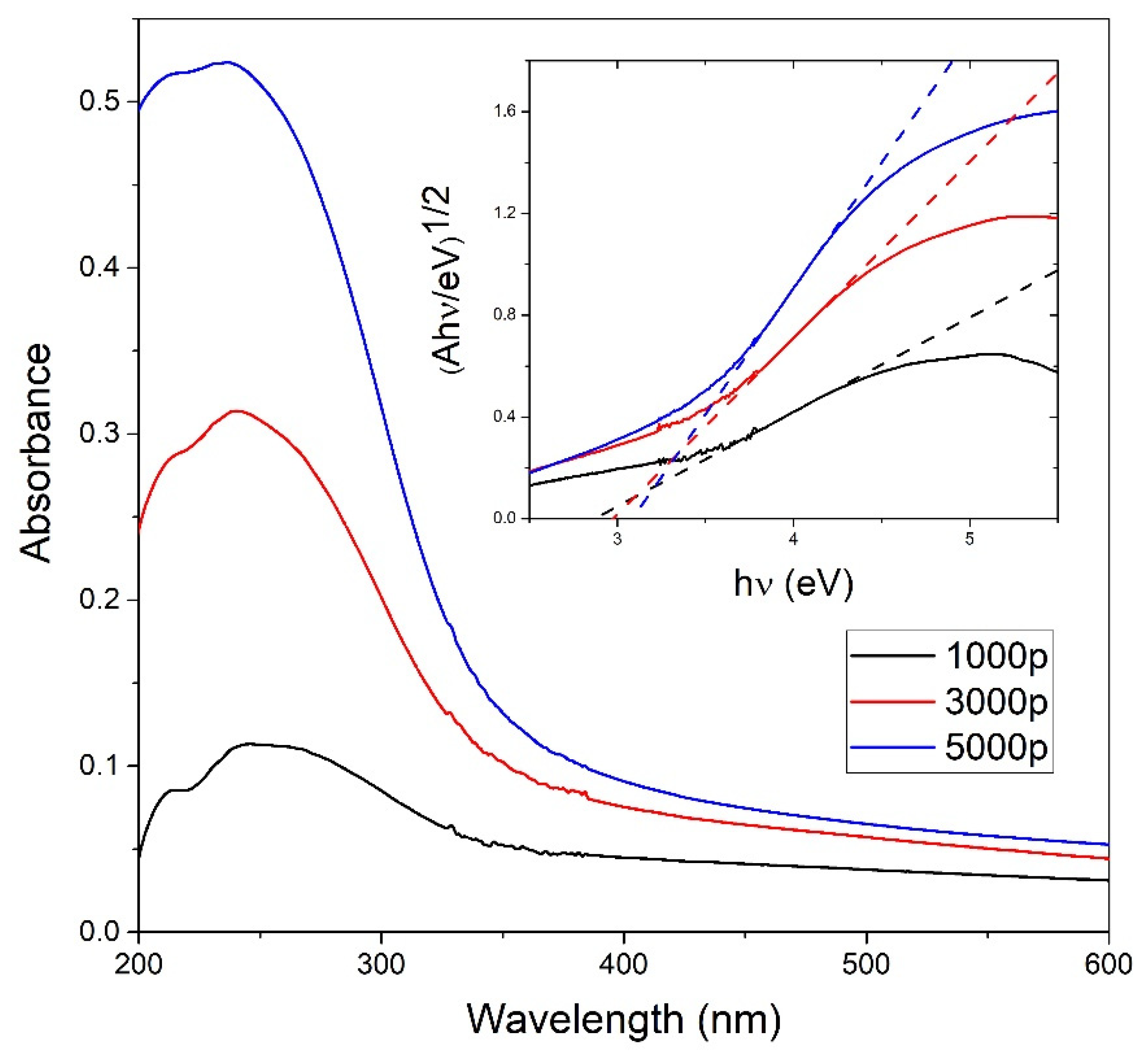
UV-Vis measurements shown in Figure 4 are performed to obtain the concentration CA of TiO2 NP in colloidal solution using the Beer–Lambert law. Indirect bandgap energies for each TiO2 colloidal solution are calculated from the photoabsorbance measurements using the Tauc plot as shown in the inset of Figure 4, and their values are 2.87 eV, 2.98 eV, and 3.08 eV for 1000, 3000, and 5000 laser pulses, respectively. The calculated indirect bandgap energies are close to the indirect bandgap energy 3.0 eV obtained in [46] for amorphous TiO2 thin films but are also close to the bandgap energies expected for the most common TiO2 phases—rutile (3.0 eV) and to a lesser extent, anatase (3.20 eV) [28].

Figure 4.
Photoabsorbance vs. wavelength measurements on TiO2 colloidal solutions dependent on the number of pulses; Inset: indirect TiO2 bandgap calculation from the Tauc plot for different colloidal TiO2 NP solutions using the photoabsorbance data.
For the calculation of the NP concentration CA from the Beer–Lambert law, the same size-distribution data (Figure 2b) was used for CV calculation. If ϕin (λ) is the entrant flux, ϕout (λ) is the output flux of light with wavelength λ through the TiO2 colloidal solution, A (λ) is the absorbance at wavelength λ, defined as in Equation (4):
If it is assumed that the colloidal solution contains spherical TiO2 NP within M different size ranges, each with a concentration ci (i = 1 to M) and average optical extinction cross-section σi (λ) within the size-range i, the absorbance A can be expressed by the Beer–Lambert law as in Equation (5):
where l = 1 cm is the absorption path length in the cuvette. In our experiment, the absorbance measurements were done immediately after the production of a colloidal solution; as such, there was no precipitation and agglomeration of TiO2 NP. From the ζ-potential measurements, it was previously concluded that the TiO2 NP colloidal solution was moderately stable. Therefore, the concentration was approximatively the same in the whole solution and can be expressed as:
where ni is abundance () of TiO2 NP in the corresponding size range. Abundance ni is calculated from the size distribution (Figure 2b) for each size range. If the expression in Equation (6) for ci is inserted in Equation (5), the following expression for concentration CA is obtained:
where is the average extinction cross-section of TiO2 NP at wavelength λ. σi (λ) is approximated with extinction cross-section σext (di, λ) corresponding to NP diameter di, which is the arithmetic mean of size-range i. The Mie theory is used for the calculation of σext (di, λ). According to the Mie theory, the extinction cross-section σext (d) of a spherical particle with diameter d is the sum of the corresponding absorption and scattering cross-section, as shown in Equation (8):
where Qext is the extinction coefficient, which is the sum of the absorption coefficient Qabs and the scattering coefficient Qscatt.
According to [47] Qext, Qscatt, Qabs can be calculated from Equations (9)–(11):
where x is the size parameter defined as:
k is the wavenumber of light in a medium (water). nmedium is a real number, due to assumed water transparency. Wavelength-dependent values for water refraction indices used in all calculations are comprehensively listed in [48,49] for water temperature 25 °C. The Mie coefficients an and bn can be calculated from Equations (13) and (14) [47]:
where jn and hn are spherical Bessel’s functions of order n. m is defined in Equation (15):
where n is the TiO2 refractive index, which is a complex number, defined as in Equation (16):
where n′ and n″ are real and imaginary parts of the refractive index, respectively.
In order to calculate wavelength dependence of TiO2 NP average extinction cross-section needed for CA calculation by Equation (7), ni values were taken from NP size distribution (Figure 2b). Equations (8)–(16) were used for the calculation of for each di, with input values of wavelength and wavelength-dependent TiO2 and H2O refractive indices. The refractive index of amorphous TiO2 is similar to the one of anatase, and rutile to a lesser extent, as obtained in [50]. Therefore, using the values of refractive indices reported in the literature for crystallized TiO2 is justified for the purpose of estimating the extinction cross-section of the TiO2 NP synthesized in this work.
To make the best estimation of , calculations were made for three different dependencies of TiO2 refractive index on wavelength found in the each of the following works: Siefke et al. [51], Sarkar et al. [52], and Bodurov et al. [53,54], which are comprehensively listed on the website [55]. Siefke et al. [51] performed the WGP (wire grid polarizer) technique for the determination of refractive indices in ALD-prepared TiO2 thin film with a thickness of 350 nm in the wavelength range of 120 nm–125 μm using TiO2 material with an indirect bandgap at 3.2 eV. Sarkar et al. [52] have used opto-plasmonic sensors for the determination of the refractive indices in TiO2 rutile thin film with a thickness of 200 nm in a wavelength range of 300 nm–1.69 μm. Bodurov et al. [53,54] used Bruggeman’s effective medium approximation for the calculation of refractive indices in TiO2 anatase nanoparticles (diameter smaller than 35 nm) dispersed in water in the wavelength range 405–635 nm; the measurements were done with a laser micro-refractometer. The calculations of Equations (8)–(16) for the determination of were performed numerically, using Matzler’s MATLAB code [39].
Figure 5 shows the wavelength-dependence of cross-sections calculated for TiO2 refractive indices from all of the three mentioned works (Siefke et al. [51], Sarkar et al. [52], Bodurov et al. [53,54]) in the wavelength range 390–600 nm. From Figure 5, it can be concluded that extinction cross-sections for all three cases are very similar to each other at wavelengths 390–415 nm, corresponding to a common TiO2 bandgap energy range 3.0–3.2 eV. For larger wavelengths, the difference between them is much greater. Therefore, Equation (7) will provide the best estimations of TiO2 NP concentration CA while inserting A(λ) and at wavelength λ that corresponds to bandgap energy. Furthermore, both the experimental absorbance A(λ) and Mie extinction cross-section have larger values and therefore lower relative error at lower wavelengths, so this is another reason why CA calculation by Equation (7) has the highest accuracy at wavelengths corresponding to bandgap energy. The third advantage of such an approach is the fact that bandgap energy is easily calculated by the Tauc plot (as in Inset of Figure 4), so it is exactly known which experimental absorbances correspond to the bandgap and should be inserted in Equation (7) for the calculation of CA. These absorbances are 0.042 for 1000p, 0.072 for 3000p, and 0.090 for 5000p.
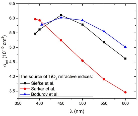
Figure 5.
Extinction cross-section dependence on wavelength calculated from the Mie theory for TiO2 solution of spherical nanoparticles using SEM size-distribution and TiO2 refractive indices from three different works: Siefke et al. [51], Sarkar et al. [52], and Bodurov et al. [53,54] (listed on the website [55]).
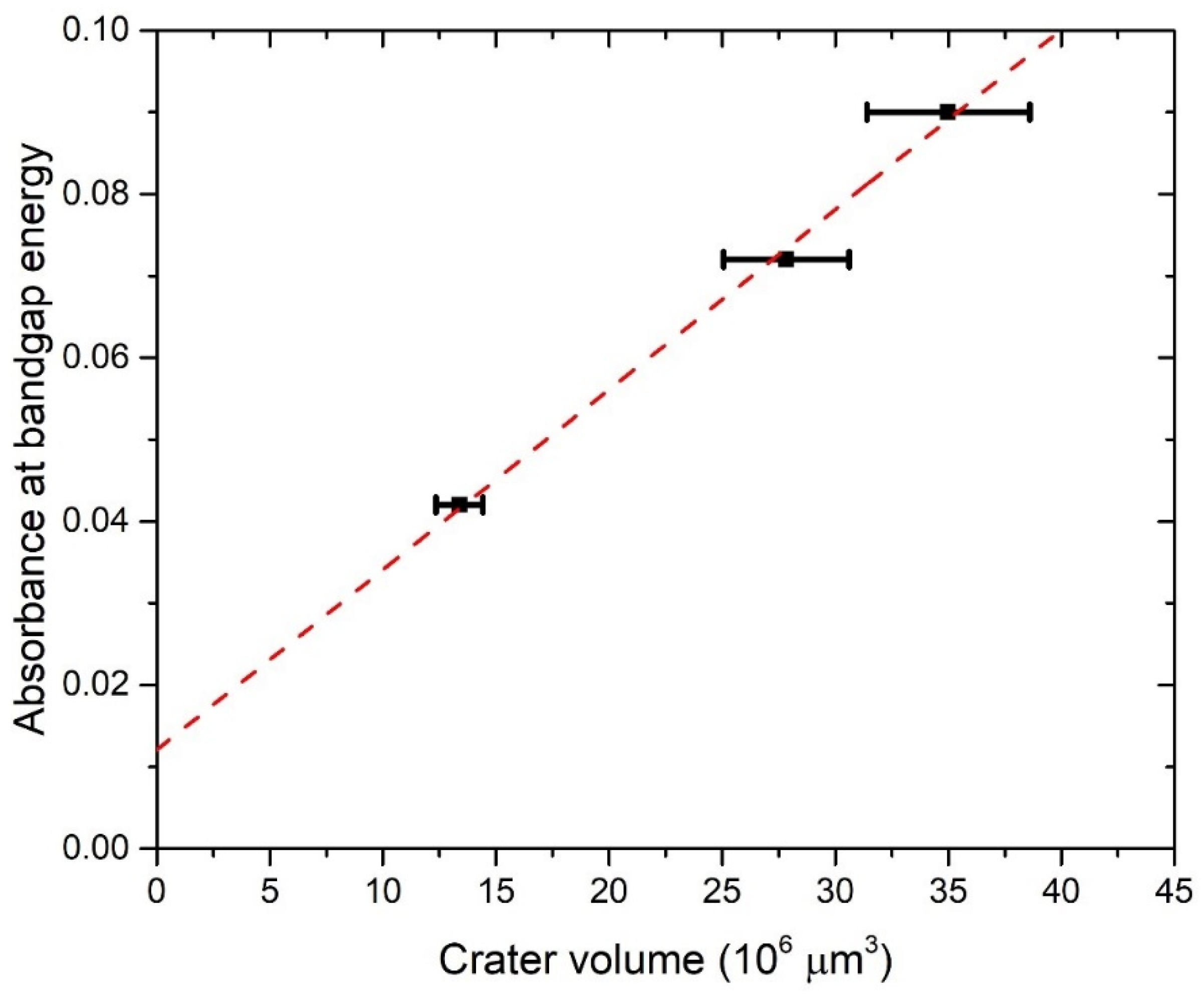
Figure 6 shows the dependence of absorbance at bandgap energy on the crater volumes. It can be seen that this dependence is linear, so it means that the average optical cross-section of TiO2 NP does not depend on the number of laser pulses. This result is expected due to the similarity in the TiO2 NP size distribution at a different number of pulses. Therefore, for each number of pulses, the same average optical cross-section can be inserted in Equation (7) for CA calculation. The extinction cross-section inserted in Equation (7) for the calculation of CA is taken from calculations made by using TiO2 refractive indices from Siefke et al. [51] and has a value of = 5.42 × 10⁻¹⁰ cm2 at wavelength 390 nm (Figure 5), which corresponds to the bandgap of TiO2 used in the same paper. The selection of the paper by Siefke et al. [51] is made due to the well-defined TiO2 bandgap, which is indirect—like the TiO2 NP in this paper. However, the difference in CA that would occur in the case of using TiO2 refractive indices from the other two papers (Sarkar et al. [52], Bodurov et al. [53,54]) is included as the contribution to the uncertainty of CA. The calculated values of concentrations CA are: CA (1000p) = (1.8 ± 0.3) × 108 mL−1, CA (3000p) = (3.1 ± 0.5) × 108 mL−1 and CA (5000p) = (3.8 ± 0.6) × 108 mL−1.
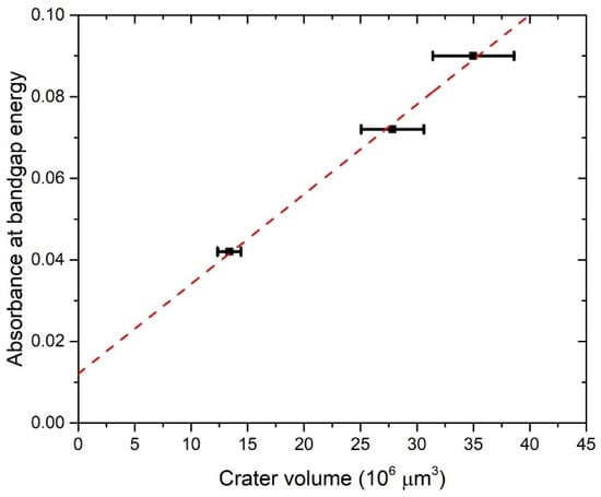
Figure 6.
The absorbance at the wavelength corresponding to the bandgap energy vs. the crater volume for TiO2 colloidal solution synthesized with PLAL. Linear fit.
4. Discussion
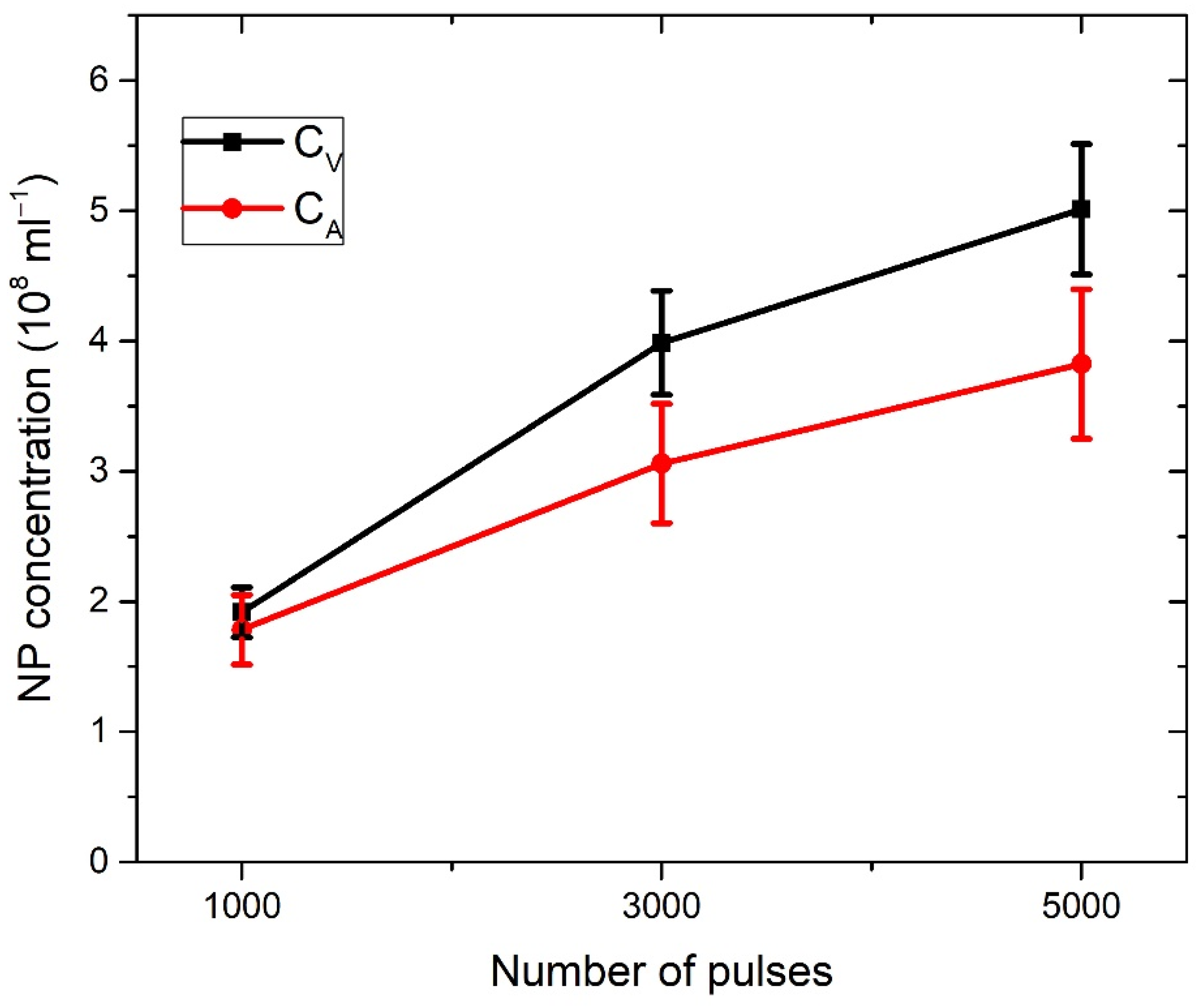
The concentrations of CV and CA as calculated here are both listed in Table 1 and shown in Figure 7 for each number of applied pulses. CA is close to CV, but slightly lower: 5% for 1000p, 22% for 3000p, and 24% for 5000p. Therefore, our proposed method for the determination of laser-synthesized TiO2 NP concentration from the size distribution and volume of the crater remained on an ablated target is verified, at least within the limits of obtained uncertainty, which are acceptable for many practical purposes.

Table 1.
TiO2 concentrations calculated from the crater volume (CV) or from the Beer–Lambert law (CA) per number of pulses.
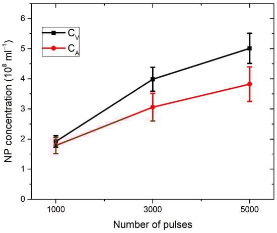
Figure 7.
Dependence of TiO2 concentration on a number of pulses for two different ways of concentration calculation using crater volume (CV) or the Beer–Lamber law (CA).
There are a few possible explanations why CA is lower than CV. First, the actual value of the optical cross-section may be smaller than the calculated value due to the multi-scattering effects that occur on TiO2 NP in colloidal solution. Second, there is a possibility that the crater volume was slightly larger than the volume of Ti material included in the formation of TiO2 NP. This was due to the crater expansion that may have occurred during the Coulomb explosion in the process of laser ablation or due to the synthesis of structures that are not observable by SEM images, like Ti ions. Third, the TiO2 NP analyzed in this paper are amorphous, so they probably have, according to [50], a slightly smaller refractive index than the one used for the calculation of σext from the paper by Siefke et al. [51]. The greatest contribution to the calculated concentration uncertainties is related to NP size-distribution uncertainty, which affects the calculation accuracy of the average volume and average optical cross-section of colloidal TiO2 NP.
The proposed method for the calculation of TiO2 NP concentration using crater volumes has significant advantages over the method using Beer–Lambert law. In the calculation of concentration using the Beer–Lambert law, a complex Mie theory is applied and, therefore, numerical calculations are needed, the NP refractive indices must be known, there usually exists the upper limit of solution density for the correct absorbance determination, the high concentration homogeneity in solution is required, and in order to have more accurate results, the angular scattering in Mie theory should be considered. These issues do not exist in the method proposed in this article for the calculation of TiO2 NP concentration from ablated crater volumes.
5. Conclusions
The method for the calculation of PLAL-synthesized NP concentration, originally introduced in our previous work [27] where it is applied for the calculation of pure metallic NP concentration (Ag NP), was herein adapted for the calculation of metal oxide NP concentration (TiO2 NP). It is based solely on the determination of the volume of an ablated material crater and the determination of the size distribution of nanoparticles. In order to verify this method, concentrations of TiO2 NP in PLAL-synthesized colloidal solutions obtained by the presented method are compared to the concentrations calculated using the Beer–Lambert law. Concentrations obtained from both methods are similar: CV is 5–25% smaller than CA in the TiO2 NP concentration range (1.8–5.0) × 108 mL−1. Therefore, it can be concluded that the proposed method is verified. This method has many advantages compared to traditional methods of concentration determination because it does not require a calibration solution, there is no uncertainty related to the nature of light interaction with nanoparticles, and the only requirement for NP size is the possibility of their detection by microscope. However, to apply this method correctly, the size distribution should be determined with high certainty because it is an important parameter that has a large impact on the calculated value of NP concentration, so this is the main limitation of this method. Furthermore, the method is not applicable when nanoparticles in colloidal solution are very inhomogeneous in terms of their stoichiometry or shape. It can be expected this method will also work for the calculation of the concentration of other metal oxide NP synthesized by PLAL and also while using other types of laser in PLAL, such as a pulsed femtosecond or microsecond laser, but further research may be carried out for confirmation.
Author Contributions
Conceptualization, D.B., J.C. and N.K.; formal analysis, D.B.; investigation, D.B. and N.K.; methodology, D.B., J.C. and N.K.; project administration, N.K.; supervision, N.K.; writing—original draft, D.B.; writing—review and editing, N.K. All authors have read and agreed to the published version of the manuscript.
Funding
This work was supported by project PZS-2019-02-5276 funded by the Croatian Science Foundation.
Institutional Review Board Statement
Not applicable.
Informed Consent Statement
Not applicable.
Data Availability Statement
Data included in the paper.
Conflicts of Interest
The authors declare no conflict of interest.
References
- Yang, G. Laser Ablation in Liquids, 1st ed.; Pan Stanford Publishing: Singapore, 2012. [Google Scholar]
- Dell’Aglio, M.; Gaudiuso, R.; De Pascale, O.; De Giacomo, A. Mechanisms and Processes of Pulsed Laser Ablation in Liquids during Nanoparticle Production. Appl. Surf. Sci. 2015, 348, 4–9. [Google Scholar] [CrossRef]
- Semaltianos, N.G. Nanoparticles by Laser Ablation. Crit. Rev. Solid State Mater. Sci. 2010, 35, 105–124. [Google Scholar] [CrossRef]
- Giorgetti, E.; Muniz Miranda, M.; Caporali, S.; Canton, P.; Marsili, P.; Vergari, C.; Giammanco, F. TiO2 Nanoparticles Obtained by Laser Ablation in Water: Influence of Pulse Energy and Duration on the Crystalline Phase. J. Alloys Compd. 2015, 643, S75–S79. [Google Scholar] [CrossRef]
- Gentile, L.; Mateos, H.; Mallardi, A.; Dell’Aglio, M.; De Giacomo, A.; Cioffi, N.; Palazzo, G. Gold Nanoparticles Obtained by Ns-Pulsed Laser Ablation in Liquids (Ns-PLAL) Are Arranged in the Form of Fractal Clusters. J. Nanopart. Res. 2021, 23, 35. [Google Scholar] [CrossRef]
- Hahn, A.; Barcikowski, S.; Chichkov, B.N. Influences on Nanoparticle Production during Pulsed Laser Ablation. J. Laser Micro/Nanoeng. 2007, 3, 73–77. [Google Scholar] [CrossRef]
- Itina, T.E. On Nanoparticle Formation by Laser Ablation in Liquids. J. Phys. Chem. C 2011, 115, 5044–5048. [Google Scholar] [CrossRef]
- Baati, T.; Al-Kattan, A.; Esteve, M.A.; Njim, L.; Ryabchikov, Y.; Chaspoul, F.; Hammami, M.; Sentis, M.; Kabashin, A.V.; Braguer, D. Ultrapure Laser-Synthesized Si-Based Nanomaterials for Biomedical Applications: In Vivo Assessment of Safety and Biodistribution. Sci. Rep. 2016, 6, 25400. [Google Scholar] [CrossRef] [Green Version]
- Shasha, C.; Krishnan, K.M. Nonequilibrium Dynamics of Magnetic Nanoparticles with Applications in Biomedicine. Adv. Mater. 2021, 33, 48–50. [Google Scholar] [CrossRef]
- Iqbal, S.; Fakhar-e-Alam, M.; Akbar, F.; Shafiq, M.; Atif, M.; Amin, N.; Ismail, M.; Hanif, A.; Farooq, W.A. Application of Silver Oxide Nanoparticles for the Treatment of Cancer. J. Mol. Struct. 2019, 1189, 203–209. [Google Scholar] [CrossRef]
- Buccolieri, A.; Serra, A.; Giancane, G.; Manno, D. Colloidal Solution of Silver Nanoparticles for Label-Free Colorimetric Sensing of Ammonia in Aqueous Solutions. Beilstein J. Nanotechnol. 2018, 9, 499–507. [Google Scholar] [CrossRef] [Green Version]
- Lohse, S.E.; Murphy, C.J. Applications of Colloidal Inorganic Nanoparticles: From Medicine to Energy. J. Am. Chem. Soc. 2012, 134, 15607–15620. [Google Scholar] [CrossRef] [PubMed]
- Blažeka, D.; Car, J.; Klobučar, N.; Jurov, A.; Zavašnik, J.; Jagodar, A.; Kovačević, E.; Krstulović, N. Photodegradation of Methylene Blue and Rhodamine b Using Laser-Synthesized Zno Nanoparticles. Materials 2020, 13, 4357. [Google Scholar] [CrossRef]
- Minelli, C.; Bartczak, D.; Peters, R.; Rissler, J.; Undas, A.; Sikora, A.; Sjöström, E.; Goenaga-Infante, H.; Shard, A.G. Sticky Measurement Problem: Number Concentration of Agglomerated Nanoparticles. Langmuir 2019, 35, 4927–4935. [Google Scholar] [CrossRef] [PubMed]
- Shang, J.; Gao, X. Nanoparticle Counting: Towards Accurate Determination of the Molar Concentration. Chem. Soc. Rev. 2014, 43, 7267–7278. [Google Scholar] [CrossRef] [PubMed] [Green Version]
- Vysotskii, V.V.; Uryupina, O.Y.; Gusel’Nikova, A.V.; Roldugin, V.I. On the Feasibility of Determining Nanoparticle Concentration by the Dynamic Light Scattering Method. Colloid J. 2009, 71, 739–744. [Google Scholar] [CrossRef]
- Ribeiro, L.N.D.M.; Couto, V.M.; Fraceto, L.F.; De Paula, E. Use of Nanoparticle Concentration as a Tool to Understand the Structural Properties of Colloids. Sci. Rep. 2018, 8, 1–8. [Google Scholar] [CrossRef] [Green Version]
- Irache, J.M.; Durrer, C.; Ponchel, G.; Duchêne, D. Determination of Particle Concentration in Latexes by Turbidimetry. Int. J. Pharm. 1993, 90, 93–96. [Google Scholar] [CrossRef]
- Xu, X.; Franke, T.; Schilling, K.; Sommerdijk, N.A.J.M.; Cölfen, H. Binary Colloidal Nanoparticle Concentration Gradients in a Centrifugal Field at High Concentration. Nano Lett. 2019, 19, 1136–1142. [Google Scholar] [CrossRef]
- Schmoll, L.H.; Peters, T.M.; O’Shaughnessy, P.T. Use of a Condensation Particle Counter and an Optical Particle Counter to Assess the Number Concentration of Engineered Nanoparticles. J. Occup. Environ. Hyg. 2010, 7, 535–545. [Google Scholar] [CrossRef]
- Tong, M.; Brown, O.S.; Stone, P.R.; Cree, L.M.; Chamley, L.W. Flow Speed Alters the Apparent Size and Concentration of Particles Measured Using NanoSight Nanoparticle Tracking Analysis. Placenta 2016, 38, 29–32. [Google Scholar] [CrossRef]
- Bachurski, D.; Schuldner, M.; Nguyen, P.H.; Malz, A.; Reiners, K.S.; Grenzi, P.C.; Babatz, F.; Schauss, A.C.; Hansen, H.P.; Hallek, M.; et al. Extracellular Vesicle Measurements with Nanoparticle Tracking Analysis–An Accuracy and Repeatability Comparison between NanoSight NS300 and ZetaView. J. Extracell. Vesicles 2019, 8, 1596016. [Google Scholar] [CrossRef] [PubMed]
- Fréchette-Viens, L.; Hadioui, M.; Wilkinson, K.J. Quantification of ZnO Nanoparticles and Other Zn Containing Colloids in Natural Waters Using a High Sensitivity Single Particle ICP-MS. Talanta 2019, 200, 156–162. [Google Scholar] [CrossRef]
- Haiss, W.; Thanh, N.T.K.; Aveyard, J.; Fernig, D.G. Determination of Size and Concentration of Gold Nanoparticles from UV-Vis Spectra. Anal. Chem. 2007, 79, 4215–4221. [Google Scholar] [CrossRef]
- Contreras, E.M.C.; Filho, E.P.B. Heat transfer performance of an automotive radiator with MWCNT nanofluid cooling in a high operating temperature range. Appl. Therm. Eng. 2022, 207, 118149. [Google Scholar] [CrossRef]
- Kozak, D.; Anderson, W.; Vogel, R.; Trau, M. Advances in Resistive Pulse Sensors: Devices Bridging the Void between Molecular and Microscopic Detection. Nano Today 2011, 6, 531–545. [Google Scholar] [CrossRef] [PubMed] [Green Version]
- Car, J.; Blažeka, D.; Bajan, T.; Krce, L.; Aviani, I.; Krstulović, N. A quantitative analysis of colloidal solution of metal nanoparticles produced by laser ablation in liquids. Appl. Phys. A 2021, 127, 838. [Google Scholar] [CrossRef]
- Lan, Y.; Lu, Y.; Ren, Z. Mini Review on Photocatalysis of Titanium Dioxide Nanoparticles and Their Solar Applications. Nano Energy 2013, 2, 1031–1045. [Google Scholar] [CrossRef]
- Sun, S.; Song, P.; Cui, J.; Liang, S. Amorphous TiO2 Nanostructures: Synthesis, Fundamental Properties and Photocatalytic Applications. Catal. Sci. Technol. 2019, 9, 4198–4215. [Google Scholar] [CrossRef]
- Wiśniewski, M.; Roszek, K. Underestimated Properties of Nanosized Amorphous Titanium Dioxide. Int. J. Mol. Sci. 2022, 23, 2460. [Google Scholar] [CrossRef]
- Vargas, M.A.; Rodríguez-Páez, J.E. Amorphous TiO2 Nanoparticles: Synthesis and Antibacterial Capacity. J. Non-Cryst. Solids 2017, 459, 192–205. [Google Scholar] [CrossRef]
- Liu, X.; Atwater, M.; Wang, J.; Huo, Q. Extinction Coefficient of Gold Nanoparticles with Different Sizes and Different Capping Ligands. Colloids Surf. B Biointerfaces 2007, 58, 3–7. [Google Scholar] [CrossRef] [PubMed]
- Hendel, T.; Wuithschick, M.; Kettemann, F.; Birnbaum, A.; Rademann, K.; Polte, J. In Situ Determination of Colloidal Gold Concentrations with Uv-Vis Spectroscopy: Limitations and Perspectives. Anal. Chem. 2014, 86, 11115–11124. [Google Scholar] [CrossRef]
- Thiele, E.S.; French, R.H. Light-Scattering Properties of Representative, Morphological Rutile Titania Particles Studied Using a Finite-Element Method. J. Am. Ceram. Soc. 2005, 81, 469–479. [Google Scholar] [CrossRef]
- Egerton, T.A. Uv-Absorption-the Primary Process in Photocatalysis and Some Practical Consequences. Molecules 2014, 19, 18192–18214. [Google Scholar] [CrossRef] [PubMed] [Green Version]
- Krstulović, N.; Shannon, S.; Stefanuik, R.; Fanara, C. Underwater-Laser Drilling of Aluminum. Int. J. Adv. Manuf. Technol. 2013, 69, 1765–1773. [Google Scholar] [CrossRef]
- Krstulović, N.; Umek, P.; Salamon, K.; Capan, I. Synthesis of Al-doped ZnO nanoparticles by laser ablation of ZnO:Al2O3 target in water. Mater. Res. Express 2017, 4, 2053–2059. [Google Scholar] [CrossRef]
- Krstulović, N.; Milošević, S. Drilling Enhancement by Nanosecond-Nanosecond Collinear Dual-Pulse Laser Ablation of Titanium in Vacuum. Appl. Surf. Sci. 2010, 256, 4142–4148. [Google Scholar] [CrossRef]
- Mätzler, C. MATLAB Functions for Mie Scattering and Absorption. IAP Res. Rep. 2002, 1139–1151. [Google Scholar]
- Krstulović, N.; Salamon, K.; Budimlija, O.; Kovač, J.; Dasović, J.; Umek, P.; Capan, I. Parameters Optimization for Synthesis of Al-Doped ZnO Nanoparticles by Laser Ablation in Water. Appl. Surf. Sci. 2018, 440, 916–925. [Google Scholar] [CrossRef]
- Mafuné, F.; Kohno, J.Y.; Takeda, Y.; Kondow, T.; Sawabe, H. Formation of Gold Nanoparticles by Laser Ablation in Aqueous Solution of Surfactant. J. Phys. Chem. B 2001, 105, 5114–5120. [Google Scholar] [CrossRef]
- Zeng, H.; Du, X.W.; Singh, S.C.; Kulinich, S.A.; Yang, S.; He, J.; Cai, W. Nanomaterials via Laser Ablation/Irradiation in Liquid: A Review. Adv. Funct. Mater. 2012, 22, 1333–1353. [Google Scholar] [CrossRef]
- Zhang, D.; Liu, J.; Li, P.; Tian, Z.; Liang, C. Recent Advances in Surfactant-Free, Surface-Charged, and Defect-Rich Catalysts Developed by Laser Ablation and Processing in Liquids. ChemNanoMat 2017, 3, 512–533. [Google Scholar] [CrossRef]
- Nakamura, T.; Ichitsubo, T.; Matsubara, E.; Muramatsu, A.; Sato, N.; Takahashi, H. On the Preferential Formation of Anatase in Amorphous Titanium Oxide Film. Scr. Mater. 2005, 53, 1019–1023. [Google Scholar] [CrossRef]
- Papanicolaou, G.C.; Kostopoulos, V.; Kontaxis, L.C.; Kollia, E.; Kotrotsos, A. A comparative study between epoxy/Titania micro- and nanoparticulate composites thermal and mechanical behavior by means of particle-matrix interphase considerations. Polym. Eng. Sci. 2017, 58, 1146–1154. [Google Scholar] [CrossRef]
- Naik, V.M.; Haddad, D.; Naik, R.; Benci, J.; Auner, G.W. Optical Properties of Anatase, Rutile and Amorphous Phases of TiO2 Thin Films Grown at Room Temperature by RF Magnetron Sputtering. Mater. Res. Soc. Symp. Proc. 2003, 755, 413–418. [Google Scholar] [CrossRef]
- Bohren, C.F.; Huffman, D.R. Absorption and Scattering of Light by Small Particles; Wiley: New York, NY, USA, 1983. [Google Scholar] [CrossRef] [Green Version]
- Thormählen, I.; Straub, J.; Grigull, U. Refractive Index of Water and Its Dependence on Wavelength, Temperature, and Density. J. Phys. Chem. Ref. Data 1985, 14, 933–945. [Google Scholar] [CrossRef] [Green Version]
- Schiebener, P.; Straub, J.; Sengers, L.J.M.H.; Gallagher, J.S. RI of Water and Steam as a Function of Wavelength, Temperature and Density. J. Phys. Chem. 1990, 19, 677. [Google Scholar]
- Bendavid, A.; Martin, P.J. Review of Thin Film Materials Deposition by the Filtered Cathodic Vacuum Arc Process at CSIRO. J. Aust. Ceram. Soc. 2014, 50, 86–101. [Google Scholar]
- Siefke, T.; Kroker, S.; Pfeiffer, K.; Puffky, O.; Dietrich, K.; Franta, D.; Ohlídal, I.; Szeghalmi, A.; Kley, E.B.; Tünnermann, A. Materials Pushing the Application Limits of Wire Grid Polarizers Further into the Deep Ultraviolet Spectral Range. Adv. Opt. Mater. 2016, 4, 1780–1786. [Google Scholar] [CrossRef]
- Sarkar, S.; Gupta, V.; Kumar, M.; Schubert, J.; Probst, P.T.; Joseph, J.; König, T.A.F. Hybridized Guided-Mode Resonances via Colloidal Plasmonic Self-Assembled Grating. ACS Appl. Mater. Interfaces 2019, 11, 13752–13760. [Google Scholar] [CrossRef] [PubMed] [Green Version]
- Bodurov, I.; Vlaeva, I.; Viraneva, A.; Yovcheva, T.; Sainov, S. Modified design of a laser refractometer. J. Nanosci. Nanotechnol. 2016, 16, 31–33. [Google Scholar]
- Bodurov, I.; Yovcheva, T.; Sainov, S. Refractive index investigations of nanoparticles dispersed in water. J. Phys. Conf. Ser. 2014, 558, 012062. [Google Scholar] [CrossRef] [Green Version]
- Available online: https://refractiveindex.info (accessed on 21 October 2021).


Publisher’s Note: MDPI stays neutral with regard to jurisdictional claims in published maps and institutional affiliations. |
© 2022 by the authors. Licensee MDPI, Basel, Switzerland. This article is an open access article distributed under the terms and conditions of the Creative Commons Attribution (CC BY) license (https://creativecommons.org/licenses/by/4.0/).