
Optimal Design of Reinforced Concrete Materials in Construction


Abstract
:
1. Introduction
2. Structural Design
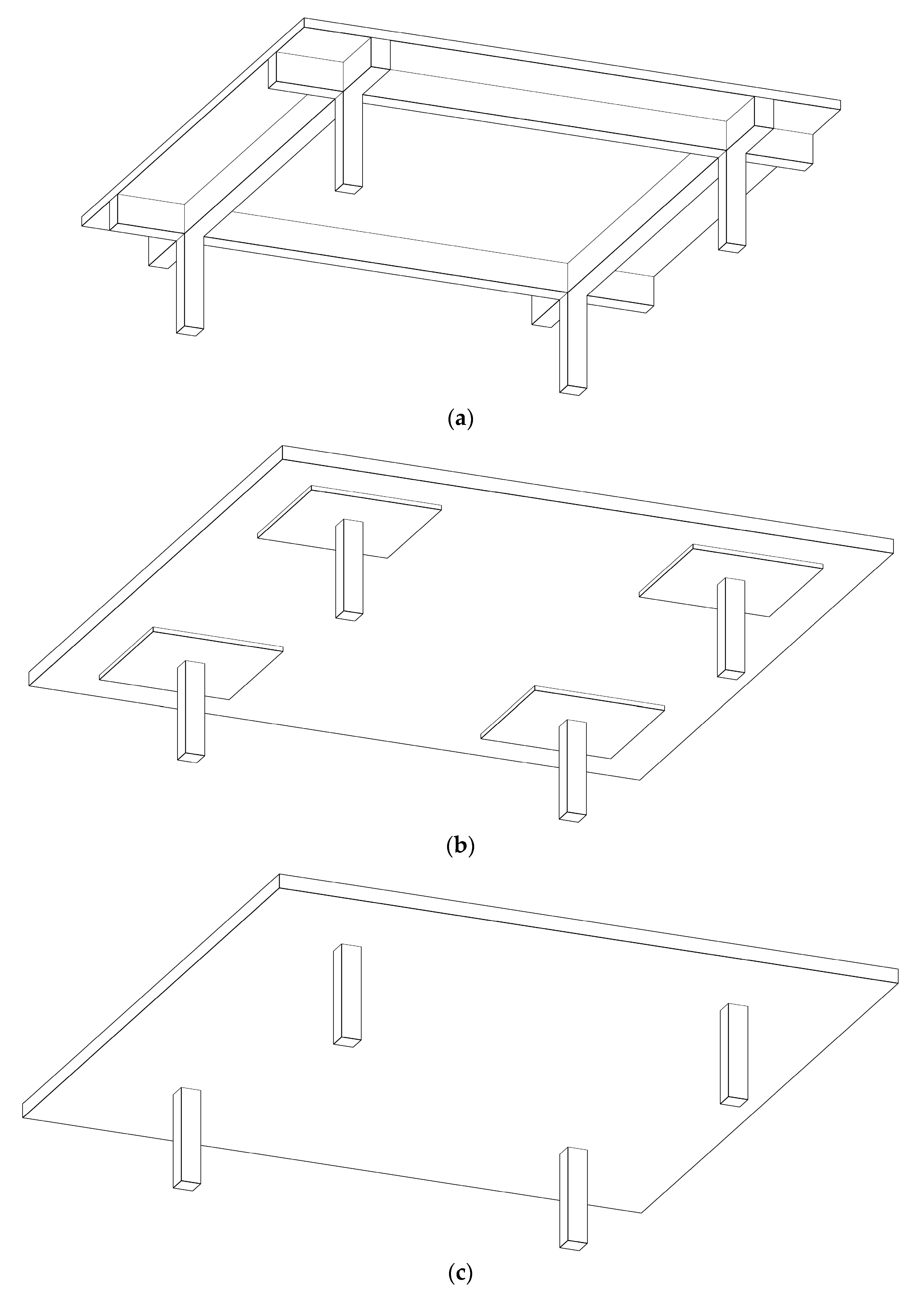
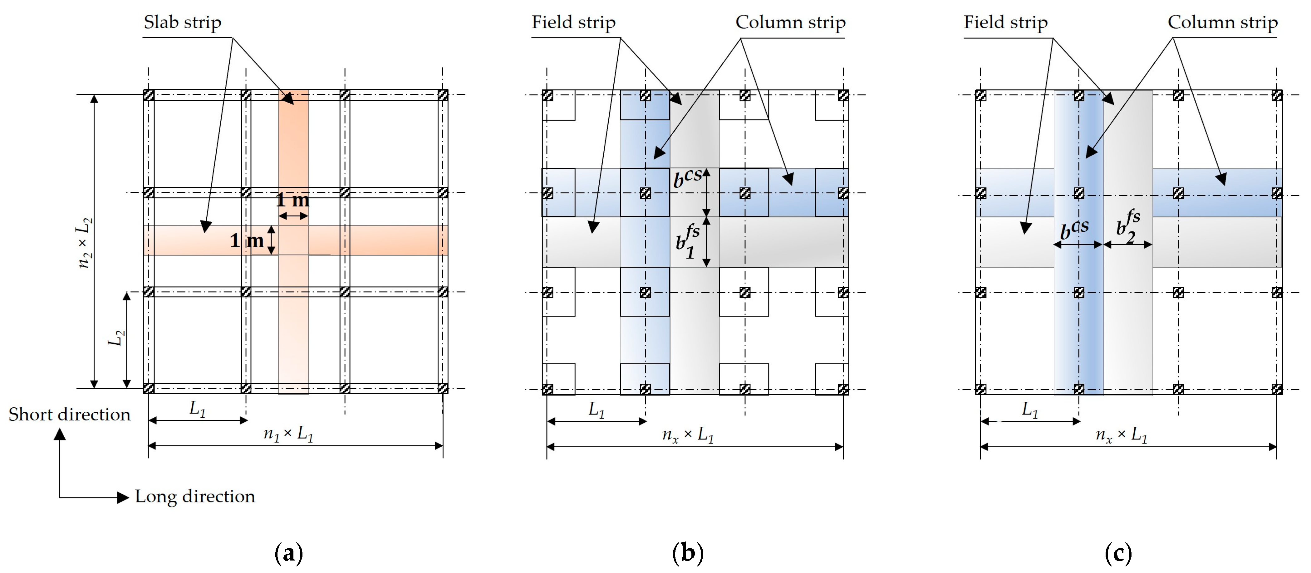
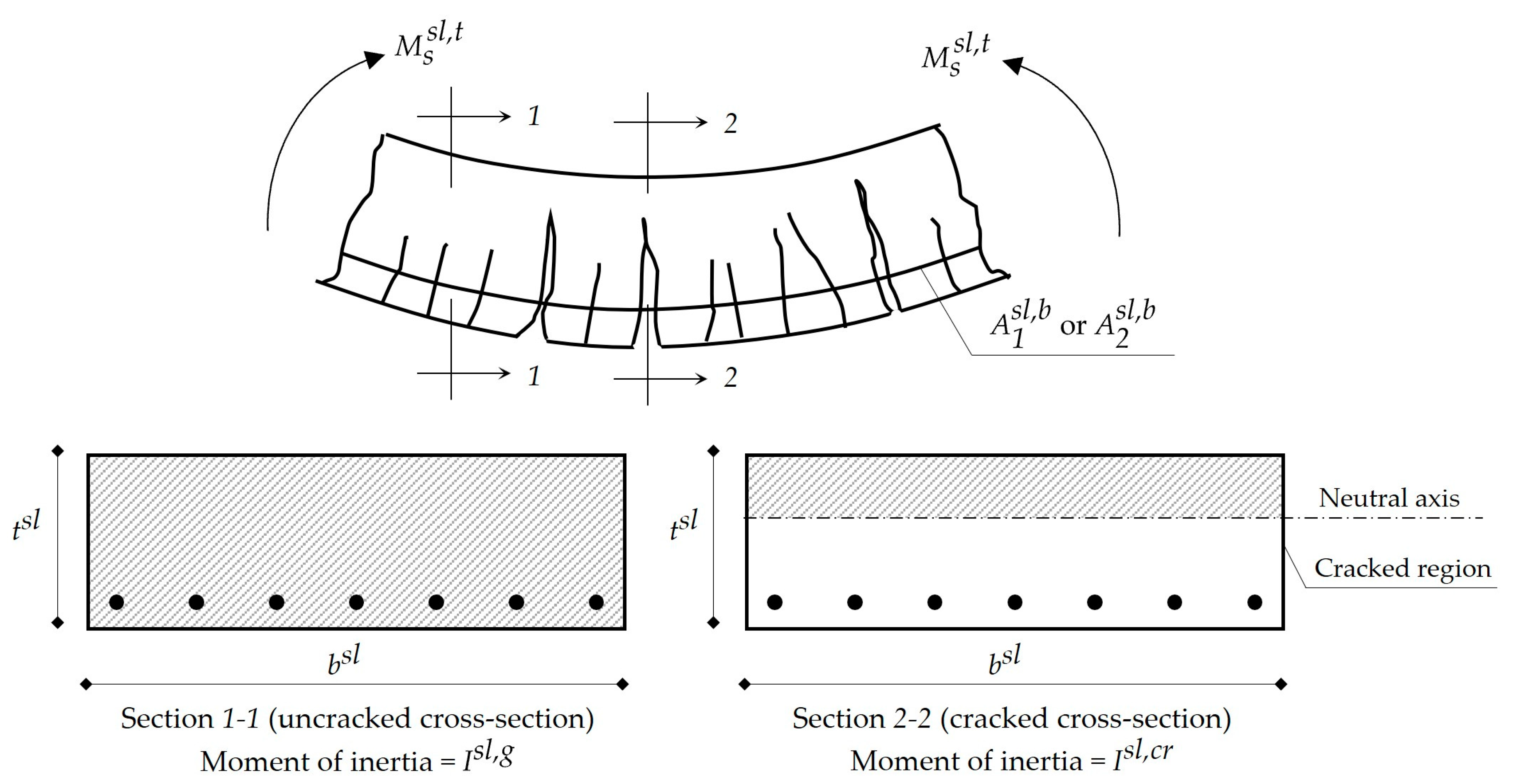
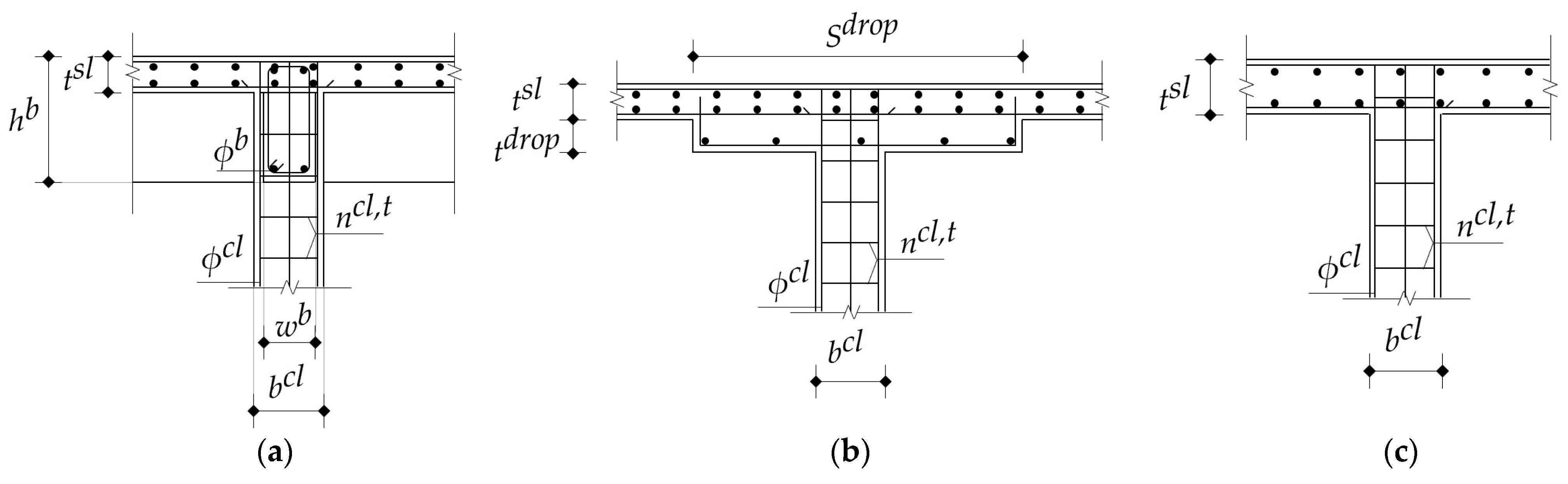
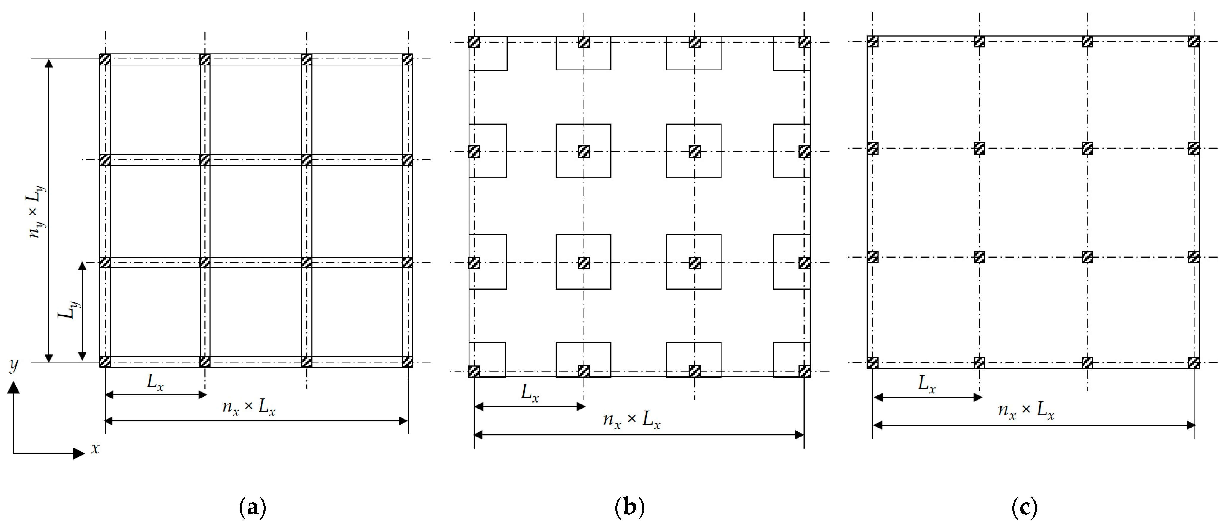
2.1. RC Slabs
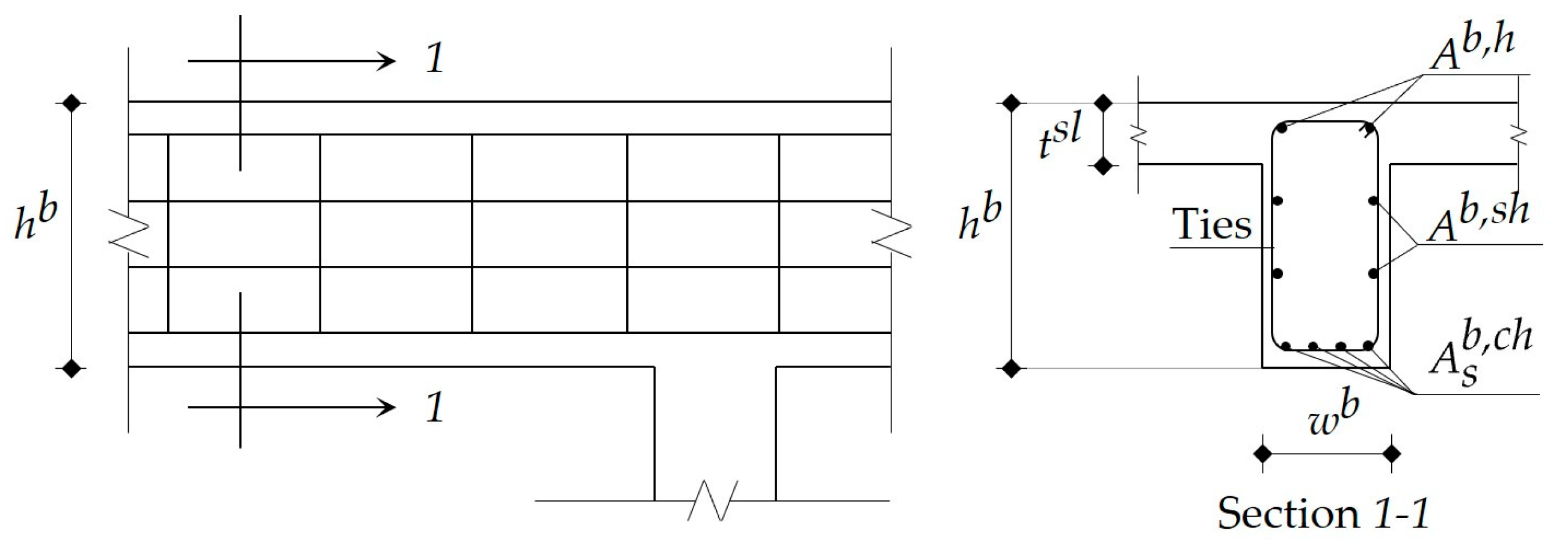
2.2. RC Beams
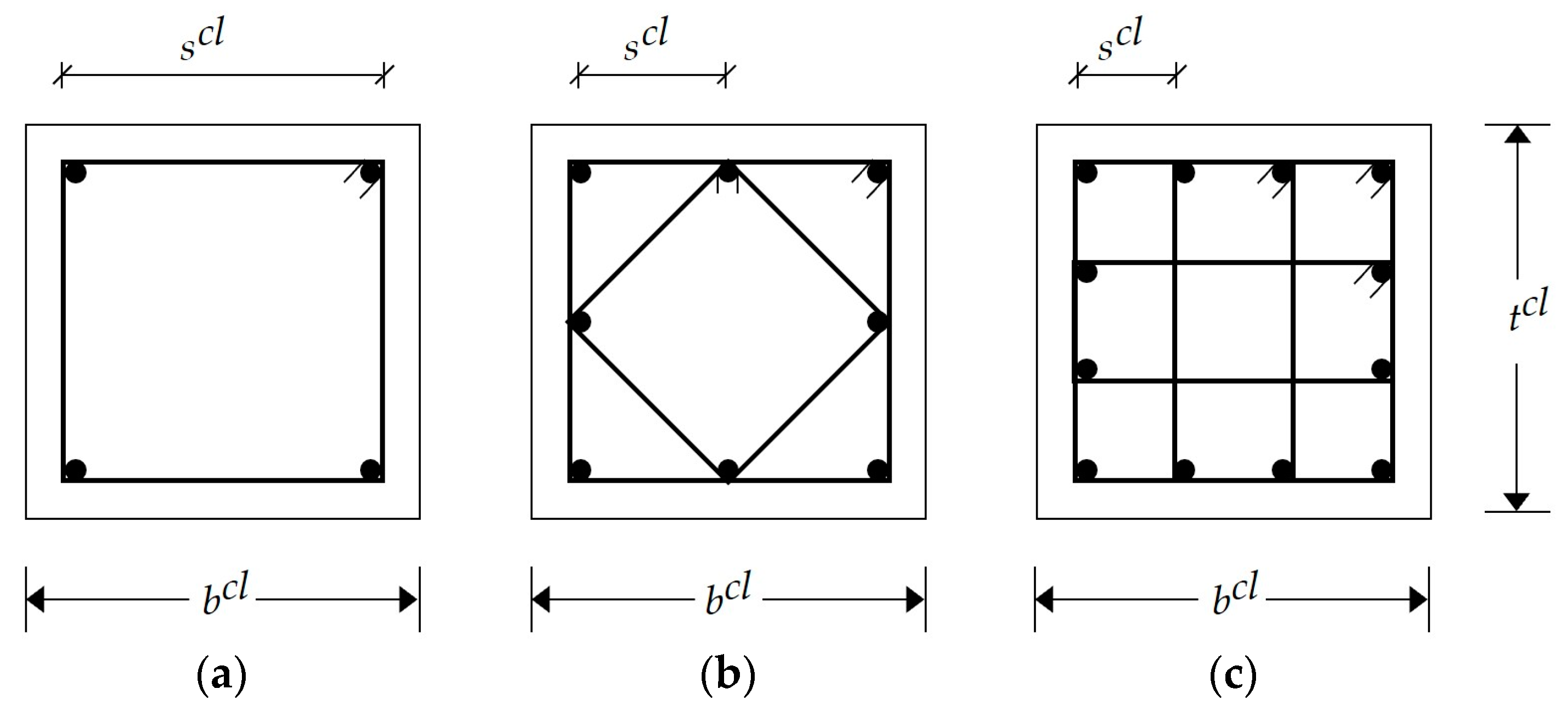
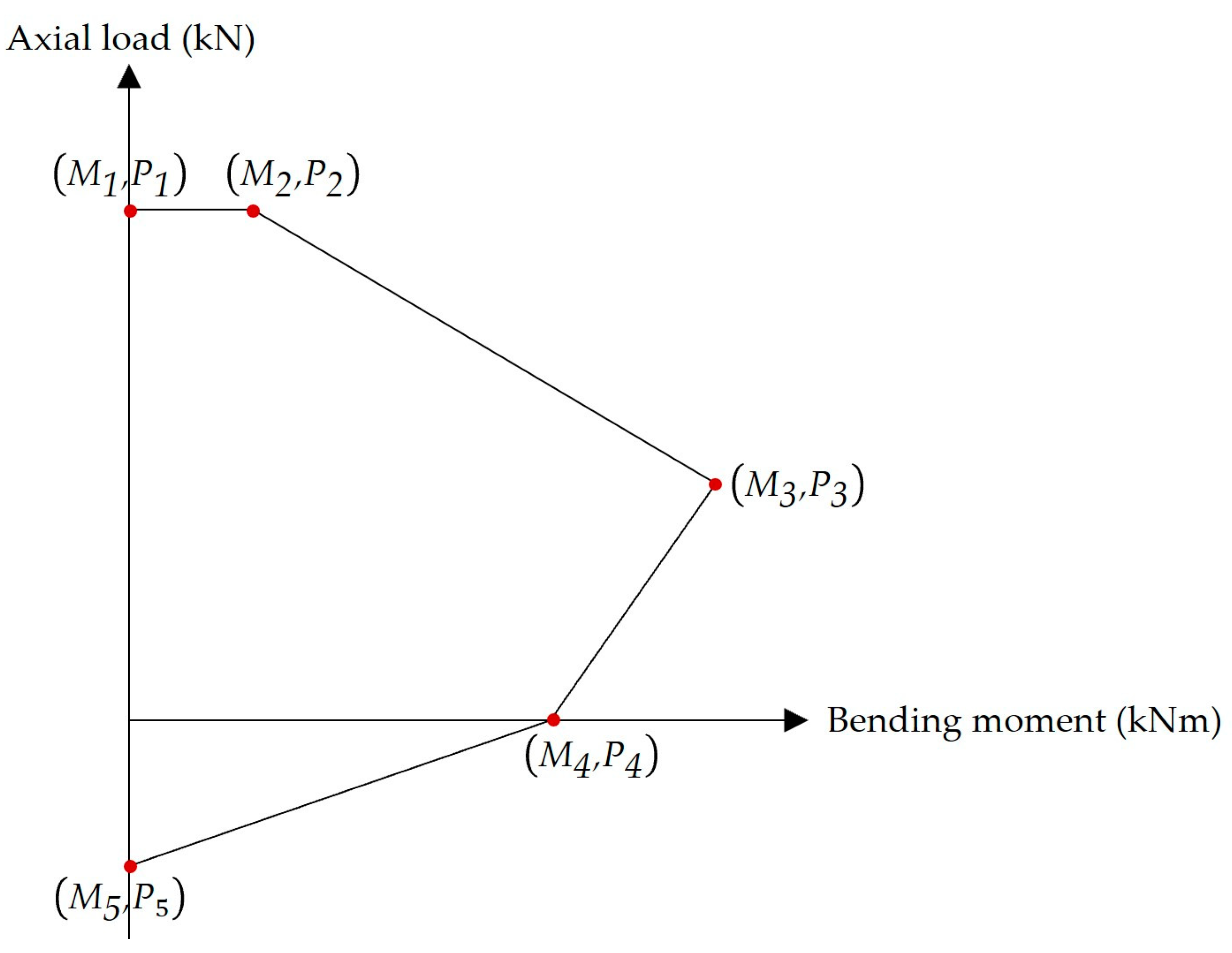
2.3. RC Columns
- Point 1 represents the pure axial compression failure mode. Here, the axial load equals .
- Point 2 represents the compression failure mode with minimum eccentricity. The bending moment can be calculated using Equation (75). The minimum eccentricity permitted by ECP 203-18 is expressed in Equation (76).
- Point 3 represents the balanced failure mode (i.e., the concrete failure and steel reinforcement yielding occur simultaneously). The axial load and the bending moment are expressed in Equations (77) and (78), respectively.where is the area of steel reinforcement on the compression side, is the area of steel reinforcement on the tension side, is the length of the equivalent rectangular stress block, is the distance from the plastic centroid to the extreme compression fibers of the column cross-section, is the distance from the center of compressive bars to the extreme compression fibers of the column cross-section, and is the distance from the center of tensile bars to the extreme compression fibers of the column cross-section.
- Point 4 represents the pure bending failure mode. The bending moment can be calculated using Equation (79).
- Point 5 represents the pure axial tension failure. The axial load can be calculated using Equation (80).
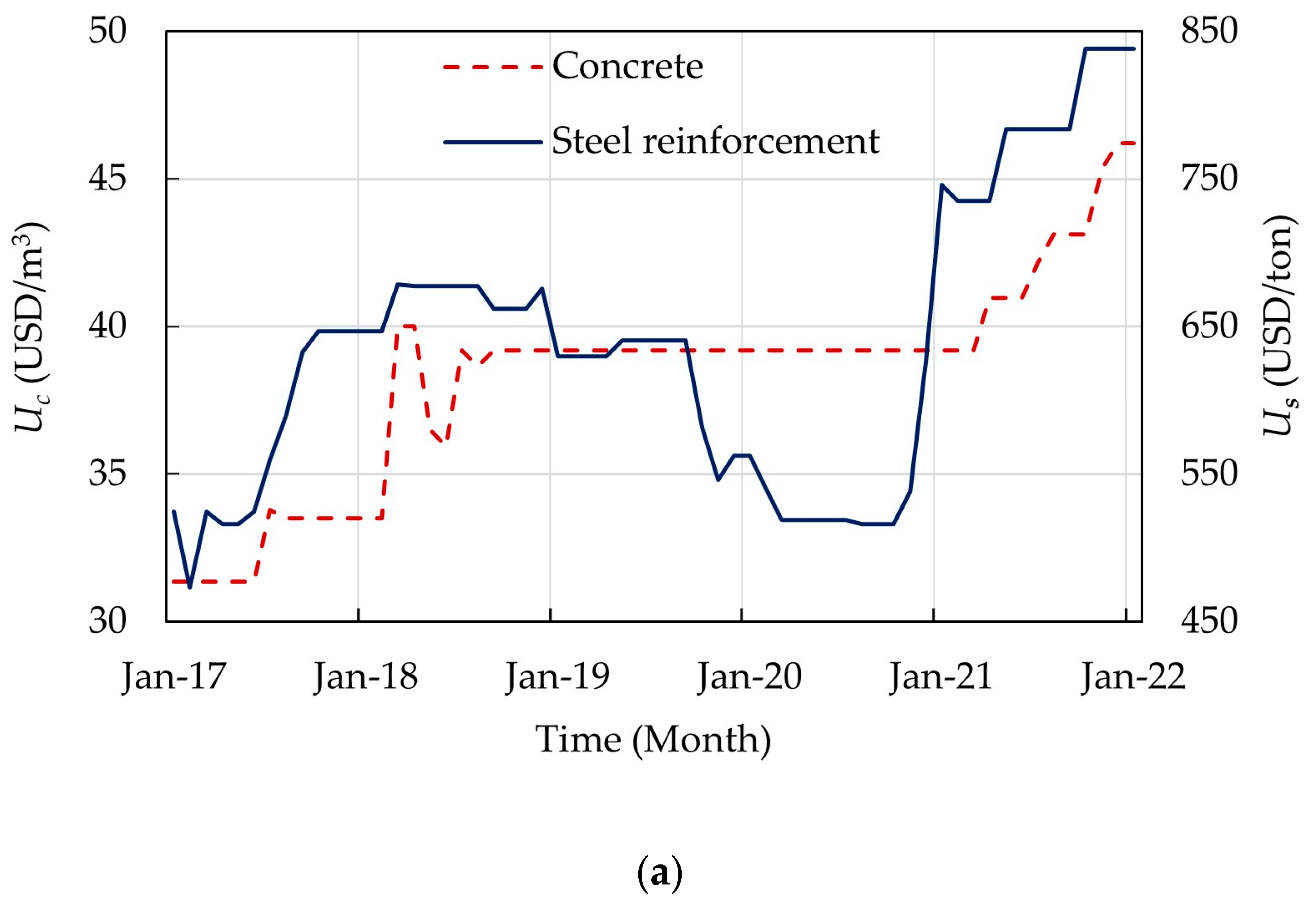
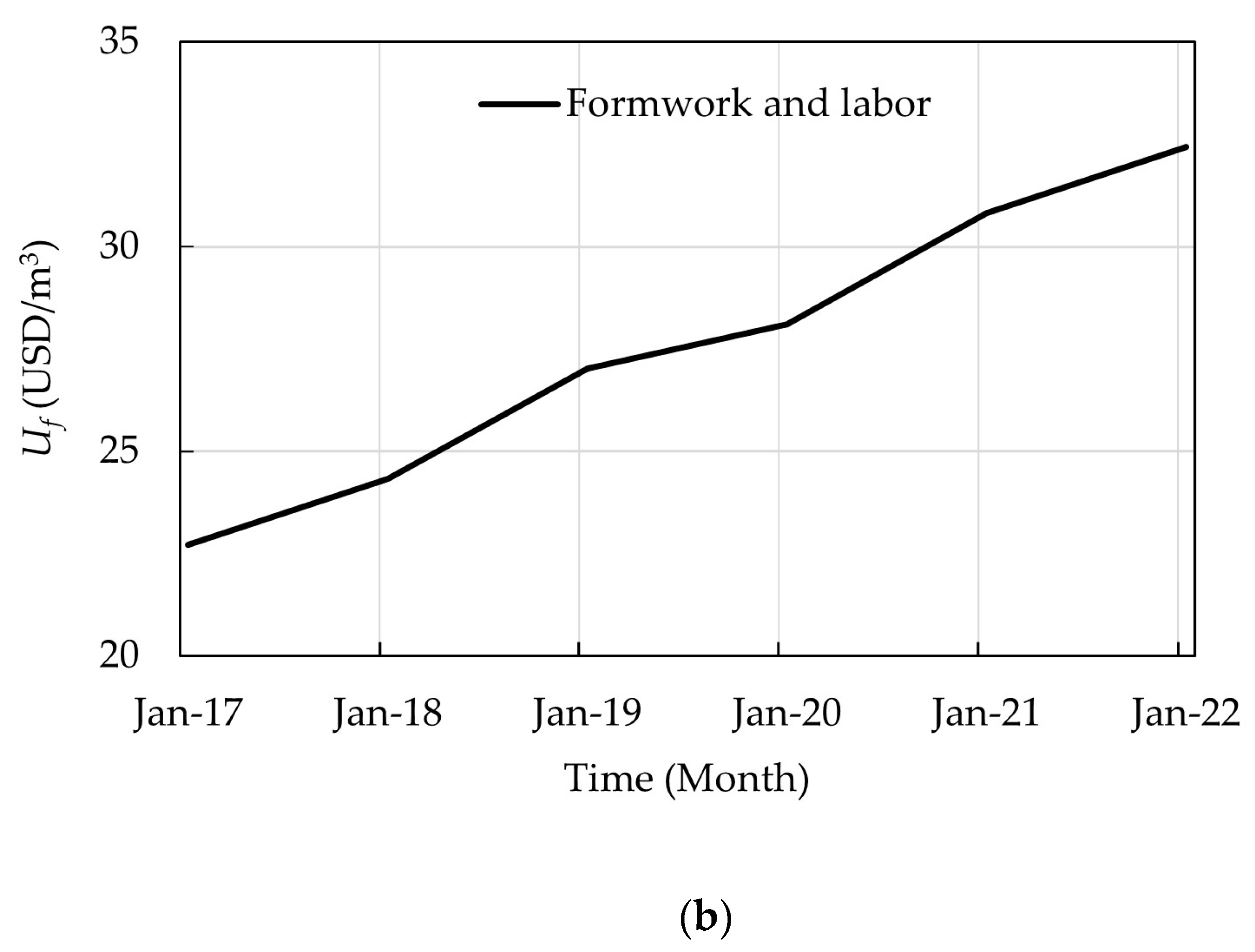
3. Construction Cost Parameters
4. Statement of the Problem
4.1. Design Variables
4.2. Objective Function
5. Optimization Algorithm
6. Benchmark Examples and Discussions
6.1. Example 1: A Four-Story Building
6.1.1. Effects of Optimizing the Concrete Grade and Column Spacings
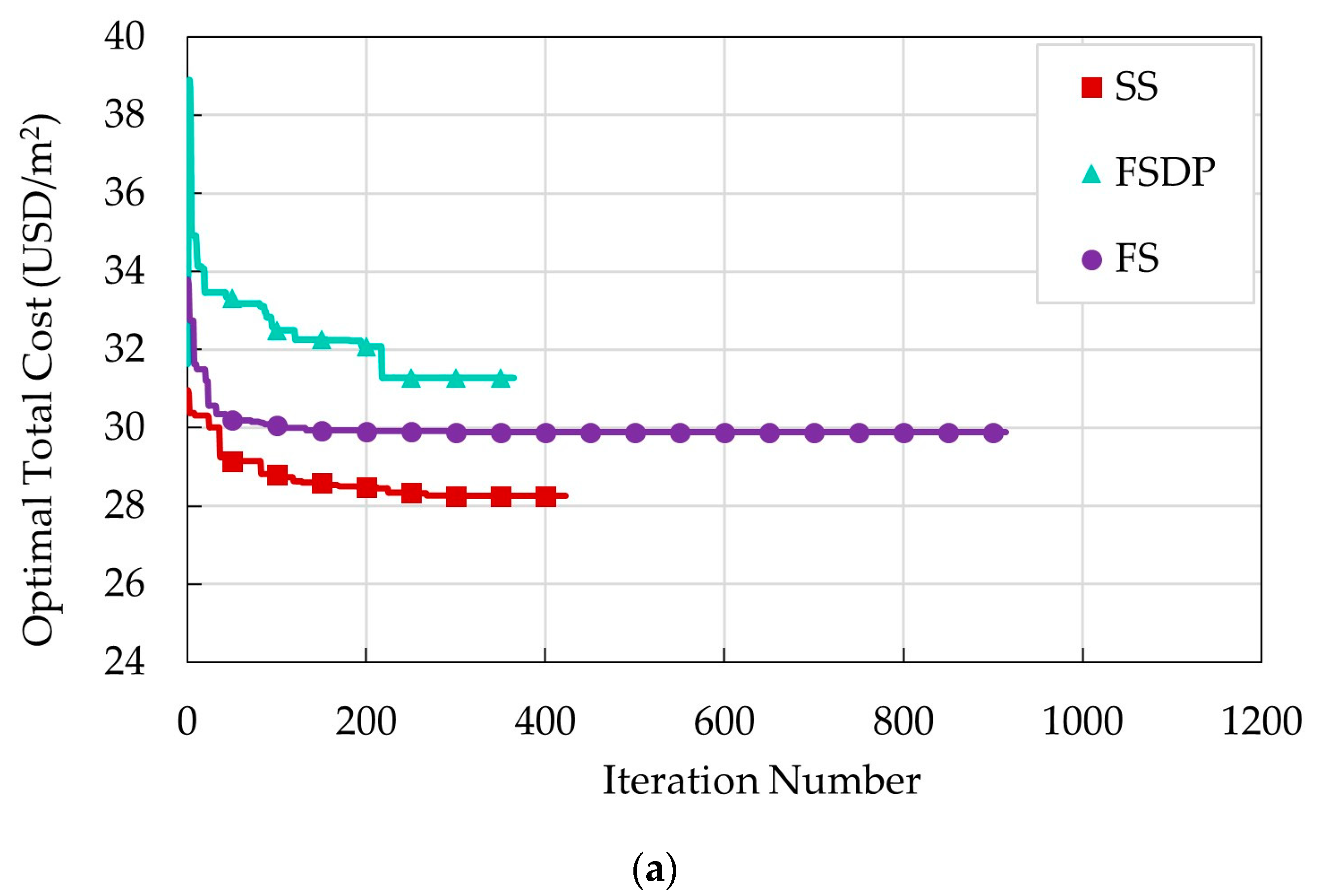
6.1.2. Comparison between Floor Systems
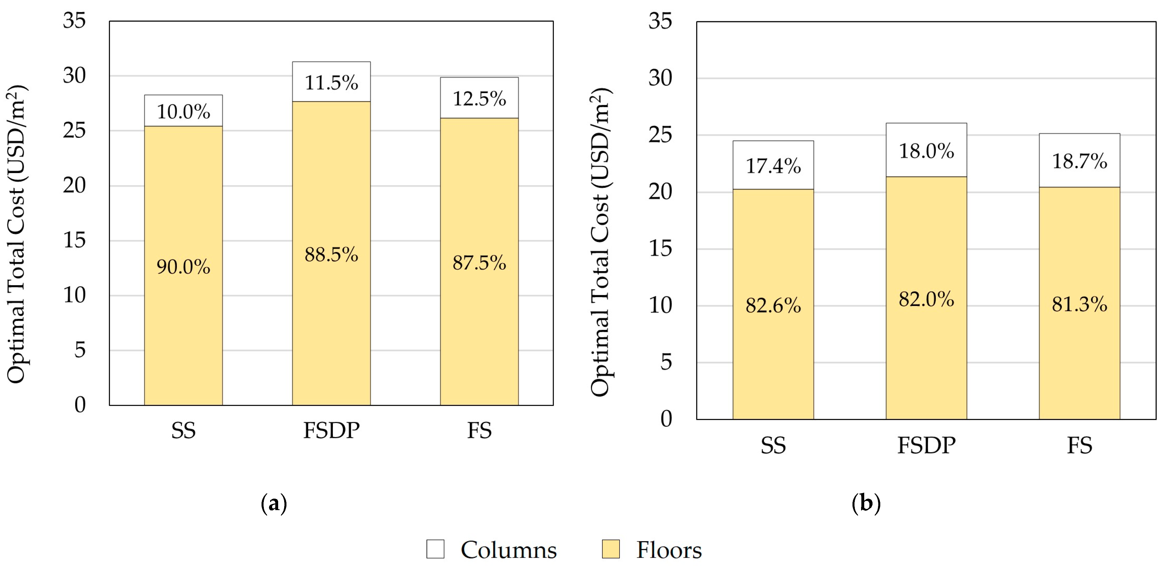
6.1.3. Distribution of Structural Elements Construction Costs
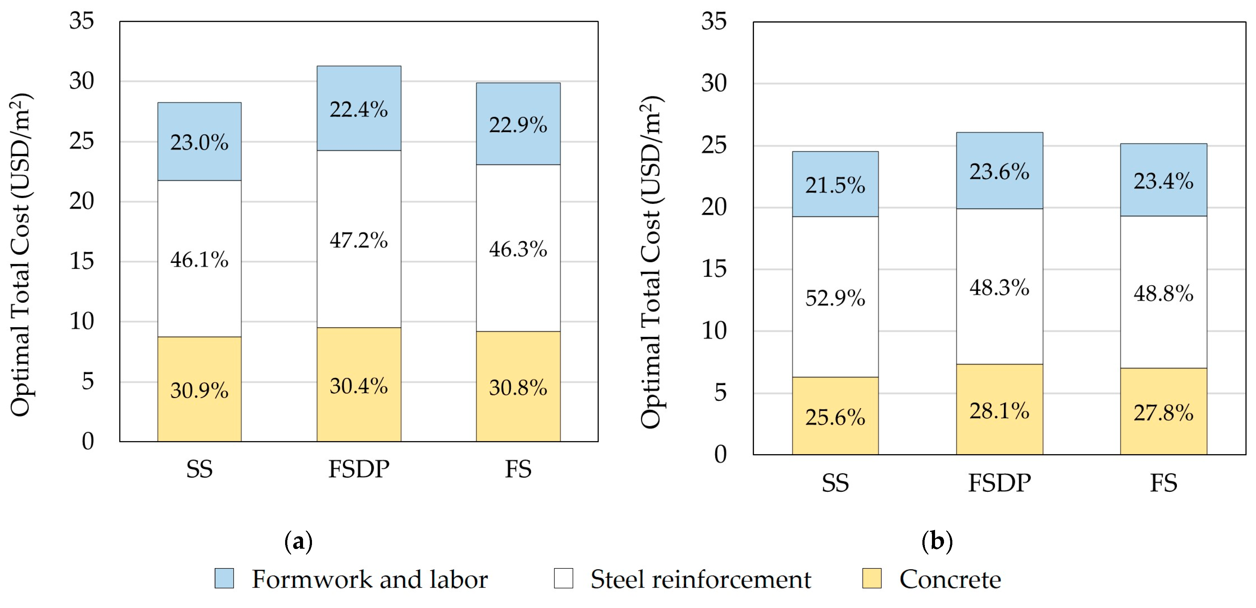
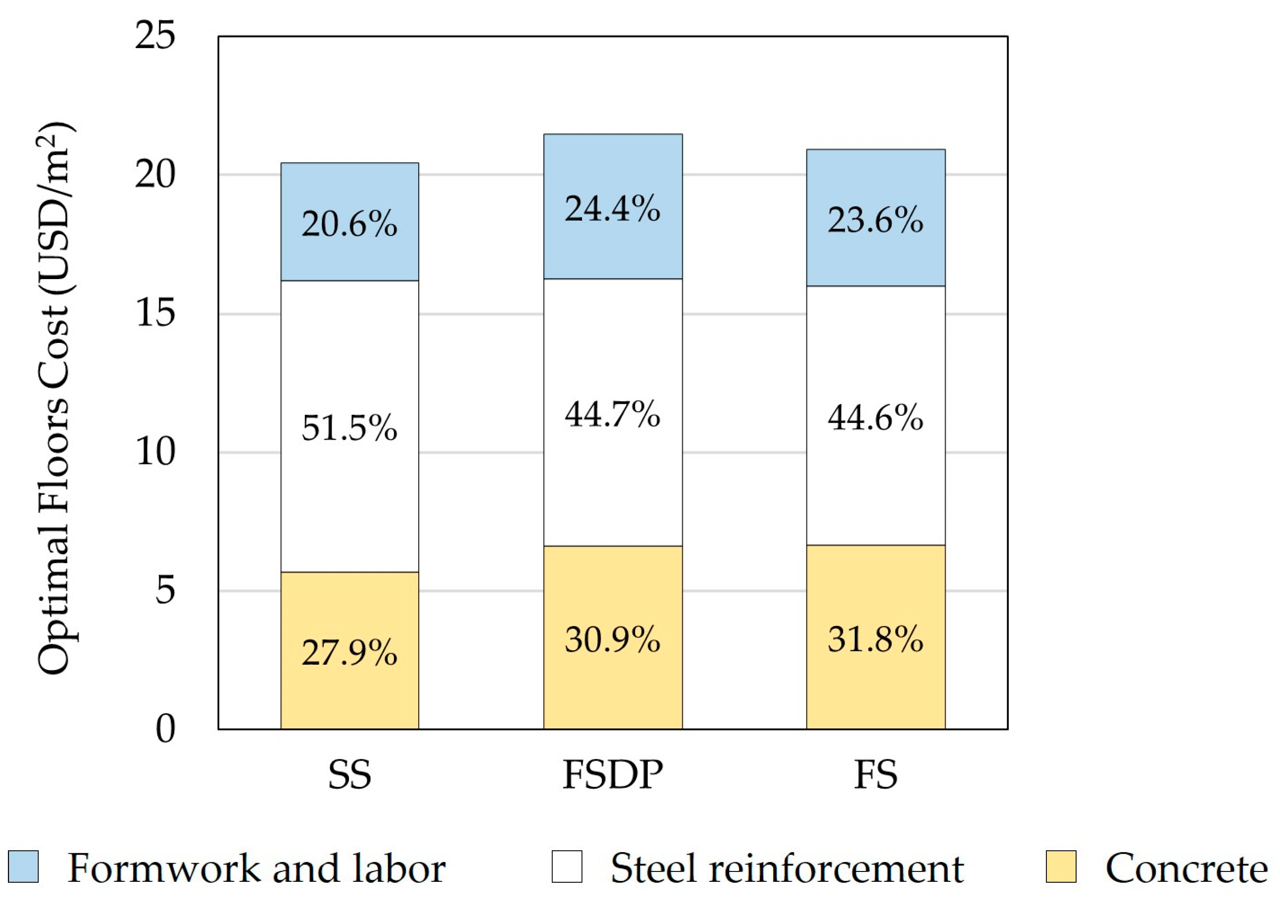
6.1.4. Distribution of Materials and Labor Construction Costs
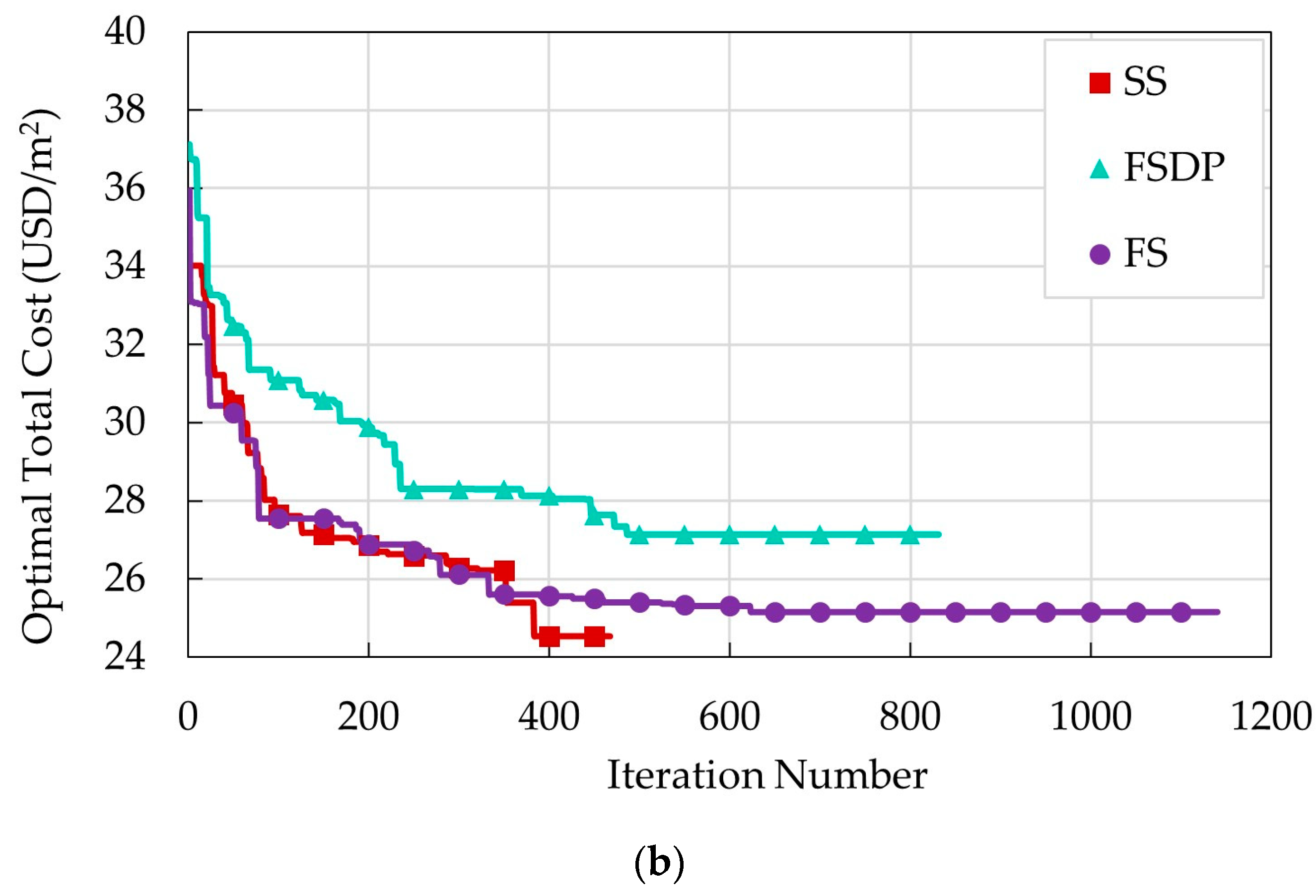
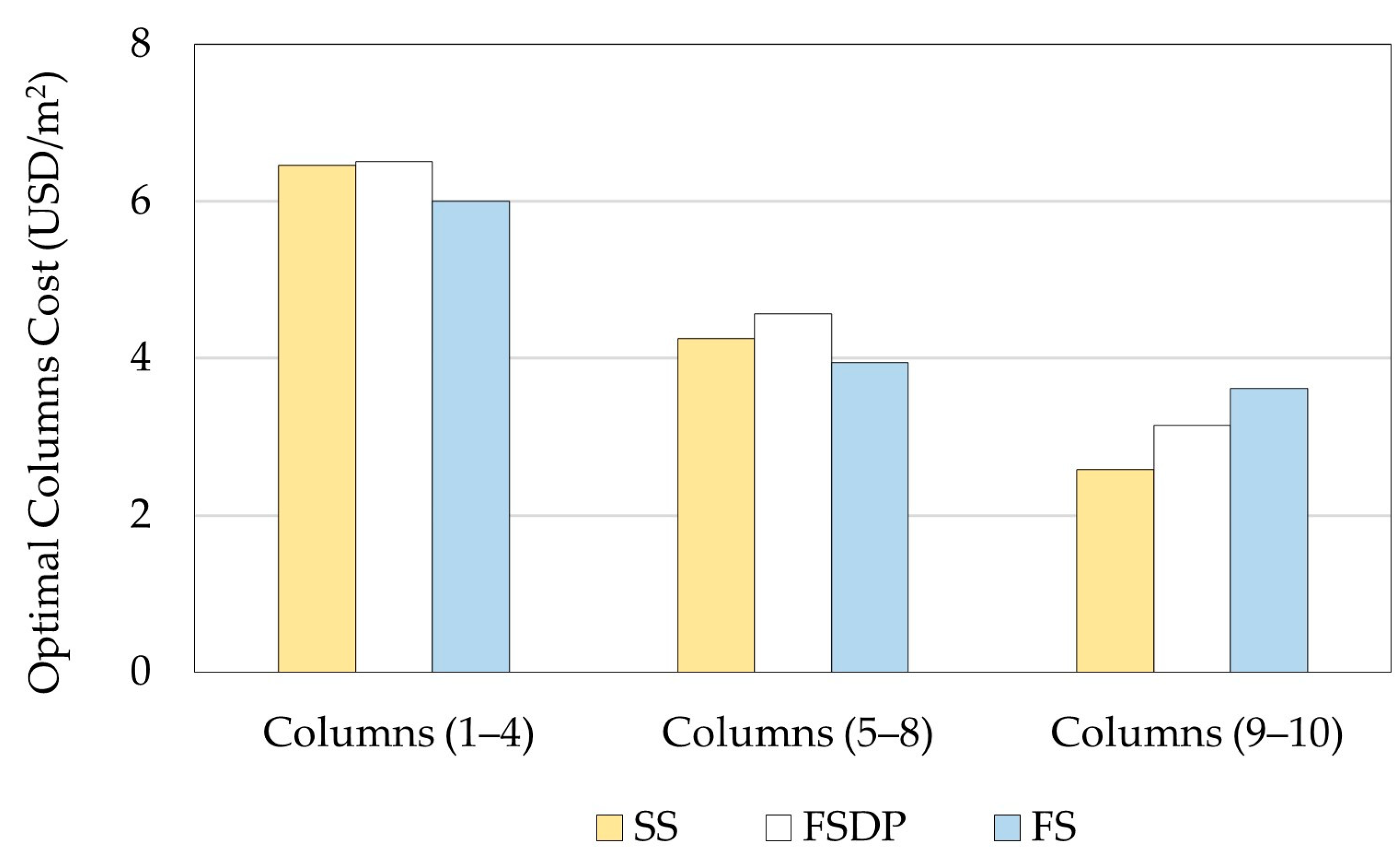
6.2. Example 2: A Ten-Story Building
7. Conclusions
Author Contributions
Funding
Institutional Review Board Statement
Informed Consent Statement
Data Availability Statement
Conflicts of Interest
References
- Serrano-González, L.; Merino-Maldonado, D.; Antolín-Rodríguez, A.; Lemos, P.C.; Pereira, A.S.; Faria, P.; Juan-Valdés, A.; García-González, J.; Morán-del Pozo, J.M. Biotreatments Using Microbial Mixed Cultures with Crude Glycerol and Waste Pinewood as Carbon Sources: Influence of Application on the Durability of Recycled Concrete. Materials 2022, 15, 1181. [Google Scholar] [CrossRef] [PubMed]
- Ashraf, M.R.; Akmal, U.; Khurram, N.; Aslam, F.; Deifalla, A.F. Impact Resistance of Styrene & ndash; Butadiene Rubber (SBR) Latex-Modified Fiber-Reinforced Concrete: The Role of Aggregate Size. Materials 2022, 15, 1283. [Google Scholar] [CrossRef] [PubMed]
- Li, Z. A Numerical Method for Applying Cohesive Stress on Fracture Process Zone in Concrete Using Nonlinear Spring Element. Materials 2022, 15, 1251. [Google Scholar] [CrossRef] [PubMed]
- Clauß, F.; Epple, N.; Ahrens, M.A.; Niederleithinger, E.; Mark, P. Correlation of Load-Bearing Behavior of Reinforced Concrete Members and Velocity Changes of Coda Waves. Materials 2022, 15, 738. [Google Scholar] [CrossRef]
- Jamshaid, H.; Mishra, R.K.; Raza, A.; Hussain, U.; Rahman, M.L.; Nazari, S.; Chandan, V.; Muller, M.; Choteborsky, R. Natural Cellulosic Fiber Reinforced Concrete: Influence of Fiber Type and Loading Percentage on Mechanical and Water Absorption Performance. Materials 2022, 15, 874. [Google Scholar] [CrossRef]
- Ji, S.-W.; Yeon, Y.-M.; Hong, K.-N. Shear Performance of RC Beams Reinforced with Fe-Based Shape Memory Alloy Stirrups. Materials 2022, 15, 1703. [Google Scholar] [CrossRef]
- Tawfik, A.B.; Mahfouz, S.Y.; Taher, S.E.-D.F. Nonlinear ABAQUS Simulations for Notched Concrete Beams. Materials 2021, 14, 7349. [Google Scholar] [CrossRef]
- Baena, M.; Barris, C.; Perera, R.; Torres, L. Influence of Bond Characterization on Load-Mean Strain and Tension Stiffening Behavior of Concrete Elements Reinforced with Embedded FRP Reinforcement. Materials 2022, 15, 799. [Google Scholar] [CrossRef]
- Bakar, M.B.C.; Muhammad Rashid, R.S.; Amran, M.; Saleh Jaafar, M.; Vatin, N.I.; Fediuk, R. Flexural Strength of Concrete Beam Reinforced with CFRP Bars: A Review. Materials 2022, 15, 1144. [Google Scholar] [CrossRef]
- de Souza, R.C.S.; Andreini, M.; La Mendola, S.; Zehfuß, J.; Knaust, C. Probabilistic Thermo-Mechanical Finite Element Analysis for the Fire Resistance of Reinforced Concrete Structures. Fire Saf. J. 2019, 104, 22–33. [Google Scholar] [CrossRef]
- Andreini, M.; Caciolai, M.; La Mendola, S.; Mazziotti, L.; Sassu, M. Mechanical Behavior of Masonry Materials at High Temperatures. Fire Mater. 2015, 39, 41–57. [Google Scholar] [CrossRef]
- Rahmanian, I.; Lucet, Y.; Tesfamariam, S. Optimal Design of Reinforced Concrete Beams: A Review. Comput. Concr. 2014, 13, 457–482. [Google Scholar] [CrossRef]
- Stochino, F.; Lopez Gayarre, F. Reinforced Concrete Slab Optimization with Simulated Annealing. Appl. Sci. 2019, 9, 3161. [Google Scholar] [CrossRef] [Green Version]
- Chutani, S.; Singh, J. Use of Modified Hybrid PSOGSA for Optimum Design of RC Frame. J. Chinese Inst. Eng. 2018, 41, 342–352. [Google Scholar] [CrossRef]
- Sánchez-Olivares, G.; Tomás, A. Optimization of Reinforced Concrete Sections under Compression and Biaxial Bending by Using a Parallel Firefly Algorithm. Appl. Sci. 2021, 11, 2076. [Google Scholar] [CrossRef]
- Bordignon, R.; Kripka, M. Optimum Design of Reinforced Concrete Columns Subjected to Uniaxial Flexural Compression. Comput. Concr. 2012, 9, 327–340. [Google Scholar] [CrossRef]
- Kripka, M.; Medeiros, G.F.; Lemonge, A.C.C. Use of Optimization for Automatic Grouping of Beam Cross-Section Dimensions in Reinforced Concrete Building Structures. Eng. Struct. 2015, 99, 311–318. [Google Scholar] [CrossRef]
- Pierott, R.; Hammad, A.W.A.; Haddad, A.; Garcia, S.; Falcón, G. A Mathematical Optimisation Model for the Design and Detailing of Reinforced Concrete Beams. Eng. Struct. 2021, 245, 112861. [Google Scholar] [CrossRef]
- Varga, R.; Žlender, B.; Jelušič, P. Multiparametric Analysis of a Gravity Retaining Wall. Appl. Sci. 2021, 11, 6233. [Google Scholar] [CrossRef]
- Habte, B.; Yilma, E. Cost Optimization of Reinforced Concrete Frames Using Genetic Algorithms. Int. J. Optim. Control Theor. Appl. 2020, 11, 59–67. [Google Scholar] [CrossRef]
- Rawat, S.; Kant Mittal, R. Optimization of Eccentrically Loaded Reinforced-Concrete Isolated Footings. Pract. Period. Struct. Des. Constr. 2018. [Google Scholar] [CrossRef]
- Correia, R.S.; Bono, G.F.F.; Bono, G. Optimization of Reinforced Concrete Beams Using Solver Tool. Rev. Ibracon Estruturas Mater. 2019, 12, 910–931. [Google Scholar] [CrossRef]
- Fernandez-Ceniceros, J.; Fernandez-Martinez, R.; Fraile-Garcia, E.; Martinez-de-Pison, F.J. Automation in Construction Decision Support Model for One-Way Floor Slab Design: A Sustainable Approach. Autom. Constr. 2013, 35, 460–470. [Google Scholar] [CrossRef]
- Ghandi, E.; Shokrollahi, N.; Nasrolahi, M. Optimum Cost Design of Reinforced Concrete Slabs Using Cuckoo Search Optimization Algorithm. Iran Univ. Sci. Technol. 2017, 7, 539–564. [Google Scholar]
- de Medeiros, G.F.; Kripka, M. Optimization of Reinforced Concrete Columns According to Different Environmental Impact Assessment Parameters. Eng. Struct. 2014, 59, 185–194. [Google Scholar] [CrossRef]
- Ukritchon, B.; Keawsawasvong, S. A Practical Method for the Optimal Design of Continuous Footing Using Ant-Colony Optimization. Acta Geotech. Slov. 2016, 13, 45–55. [Google Scholar]
- Jelušič, P.; Žlender, B. Optimal Design of Pad Footing Based on MINLP Optimization. Soils Found. 2018, 58, 277–289. [Google Scholar] [CrossRef]
- Mergos, P.E.; Mantoglou, F. Optimum Design of Reinforced Concrete Retaining Walls with the Flower Pollination Algorithm. Struct. Multidiscip. Optim. 2020, 61, 575–585. [Google Scholar] [CrossRef]
- Arama, Z.A.; Kayabekir, A.E.; Bekdaş, G.; Kim, S.; Geem, Z.W. The Usage of the Harmony Search Algorithm for the Optimal Design Problem of Reinforced Concrete Retaining Walls. Appl. Sci. 2021, 11, 1343. [Google Scholar] [CrossRef]
- Sahab, M.G.; Ashour, A.F.; Toropov, V.V. Cost Optimisation of Reinforced Concrete Flat Slab Buildings. Eng. Struct. 2005, 27, 313–322. [Google Scholar] [CrossRef]
- Ženíšek, M.; Pešta, J.; Tipka, M.; Kočí, V.; Hájek, P. Optimization of RC Structures in Terms of Cost and Environmental Impact—Case Study. Sustainability 2020, 12, 8532. [Google Scholar] [CrossRef]
- Dehnavipour, H.; Mehrabani, M.; Fakhriyat, A.; Jakubczyk-Gałczyńska, A. Optimization-Based Design of 3D Reinforced Concrete Structures. J. Soft Comput. Civ. Eng. 2019, 3, 95–106. [Google Scholar] [CrossRef]
- Boscardin, J.T.; Yepes, V.; Kripka, M. Optimization of Reinforced Concrete Building Frames with Automated Grouping of Columns. Autom. Constr. 2019, 104, 331–340. [Google Scholar] [CrossRef]
- Robati, M.; Mccarthy, T.J.; Kokogiannakis, G. Integrated Life Cycle Cost Method for Sustainable Structural Design by Focusing on a Benchmark Office Building in Australia. Energy Build. 2018, 166, 525–537. [Google Scholar] [CrossRef] [Green Version]
- ECP Committee, 203. Egyptian Code for Design and Construction of Concrete Structures (ECP 203-2018), 4th ed.; Housing and Building National Research Center: Cairo, Egypt, 2018. [Google Scholar]
- Committee, E. Egyptian Code for Calculating Loads and Forces in Structural Work and Masonry; Housing and Building National Research Center (HBRC): Giza, Egypt, 2012. [Google Scholar]
- Němec, P.; Stodola, P. Optimization of the Multi-Facility Location Problem Using Widely Available Office Software. Algorithms 2021, 14, 106. [Google Scholar] [CrossRef]
- Langdon, D. Spon’s Architects’ and Builders’ Price Book 2001, 126th ed.; Spon Press: London, UK, 2001. [Google Scholar] [CrossRef]
- Harris, E.C. CESMM3 Price Database: 1999/2000; Thomas Telford Ltd: London, UK, 1999. [Google Scholar]


| Type of Column | Interior | Edge | Corner |
|---|---|---|---|
| Shape |  |  |  |
| Critical shear length | |||
| Critical shear width | |||
| Critical shear perimeter | 2 | ||
| Critical shear area | |||
| Tributary area |
| Component | Strength (MPa) | Unit | Price (USD/Unit) | |
|---|---|---|---|---|
| Concrete | 25 | m3 | 36.8 | |
| 30 | 39.2 | |||
| 35 | 41.6 | |||
| 40 | 44.1 | |||
| 45 | 48.4 | |||
| 50 | 52.7 | |||
| 55 | 57.0 | |||
| 60 | 61.4 | |||
| High tensile steel | 420 | ton | 735.1 | |
| Mild steel | 240 | 735.1 | ||
| Formwork and labor | - | m3 | 30.8 |
| Parameter | Design Variable | Symbol | Increment/Set | Lower Bound | Upper Bound | SS | FSDP | FS |
|---|---|---|---|---|---|---|---|---|
| Concrete grade | Characteristic compressive strength | ✓ | ✓ | ✓ | ||||
| Column spacings | Number of spans (x-direction) | 1 | ✓ | ✓ | ✓ | |||
| Number of spans (y-direction) | ✓ | ✓ | ✓ | |||||
| Concrete dimensions | Slab thickness | 20 mm | ✓ | ✓ | ✓ | |||
| Beam height | 50 mm | ✓ | - | - | ||||
| Beam width | 50 mm | ✓ | - | - | ||||
| Drop panel thickness | 20 mm | - | ✓ | - | ||||
| Drop panel width | 50 mm | - | ✓ | - | ||||
| Interior column width | 50 mm | 800 mm | ✓ | ✓ | ✓ | |||
| Edge column width (x-direction) | ✓ | ✓ | ✓ | |||||
| Edge column width (y-direction) | ✓ | ✓ | ✓ | |||||
| Corner column width | ✓ | ✓ | ✓ | |||||
| Steel reinforcement | Beam bar diameter | ✓ | - | - | ||||
| Interior column bar diameter | ✓ | ✓ | ✓ | |||||
| Edge column bar diameter (x-direction) | ✓ | ✓ | ✓ | |||||
| Edge column bar diameter (y-direction) | ✓ | ✓ | ✓ | |||||
| Corner column bar diameter | ✓ | ✓ | ✓ | |||||
| Number of interior column lateral ties | 1 | ✓ | ✓ | ✓ | ||||
| Number of edge column lateral ties (x-direction) | ✓ | ✓ | ✓ | |||||
| Number of edge column lateral ties (y-direction) | ✓ | ✓ | ✓ | |||||
| Number of corner column lateral ties | ✓ | ✓ | ✓ |
| Parameter | Value |
|---|---|
| Constraint precision | 1 × 10⁻⁶ |
| Maximum time | Unrestricted |
| Iterations | Unrestricted |
| Maximum subproblems | Unrestricted |
| Maximum feasible solutions | Unrestricted |
| Convergence | 1 × 10⁻⁴ |
| Mutation rate | 0.075 |
| Population size | 100 |
| Random seed | 0 |
| Maximum time without improvement | 120 s |
| Parameter | Value | |
|---|---|---|
| Yield strength of the longitudinal steel reinforcement | 420 MPa | |
| Yield strength of the lateral steel reinforcement | 240 MPa | |
| Elastic modulus of steel | 200 GPa | |
| Unit weight of concrete | 25 kN/m3 | |
| Unit weight of steel | 78.5 kN/m3 | |
| Unit weight of brick partition walls | 14 kN/m3 | |
| Safety reduction factor for concrete | 1.5 | |
| Safety reduction factor for steel | 1.15 | |
| Concrete cover of slabs | 25 mm | |
| Concrete cover of beams | 50 mm | |
| Concrete cover of columns | 25 mm | |
| p | Live load | 2 kPa |
| Flooring load | 1.5 kPa | |
| Bar diameter of lateral steel reinforcement | 8 mm | |
| Floor System | Case | (mm) | (MPa) | (mm) | (mm) | (mm) | (mm) | (mm) | Floors Cost (USD/m2) | |
|---|---|---|---|---|---|---|---|---|---|---|
| SS | 1 | 5 | 6000 × 5000 | 35 | 140 | - | - | 500 | 250 | 25.43 |
| 2 | 8 | 3750 × 3125 | 25 | 80 | - | - | 400 | 250 | 20.25 | |
| FSDP | 1 | 5 | 6000 × 5000 | 35 | 200 | 60 | 2000 | - | - | 27.66 |
| 2 | 8 | 3750 × 3125 | 25 | 160 | 40 | 1600 | - | - | 21.36 | |
| FS | 1 | 5 | 6000 × 5000 | 35 | 200 | - | - | - | - | 26.16 |
| 2 | 8 | 3750 × 3125 | 25 | 160 | - | - | - | - | 20.46 |
| Floor System | Case | Interior Columns | Edge Columns (x-Direction) | Edge Columns (y-Direction) | Corner Columns | Columns Cost (USD/m2) | ||||||||
|---|---|---|---|---|---|---|---|---|---|---|---|---|---|---|
(mm) | Steel Bars | No. of Columns | (mm) | Steel Bars | No. of Columns | (mm) | Steel Bars | No. of Columns | (mm) | Steel Bars | No. of Columns | |||
| SS | 1 | 400 | 8T16 | 16 | 300 | 4T16 | 8 | 250 | 4T18 | 8 | 250 | 4T16 | 4 | 2.83 |
| 2 | 300 | 4T16 | 49 | 250 | 4T16 | 14 | 250 | 4T16 | 14 | 250 | 4T16 | 4 | 4.28 | |
| FSDP | 1 | 400 | 8T16 | 16 | 350 | 8T16 | 8 | 350 | 8T16 | 8 | 300 | 4T16 | 4 | 3.61 |
| 2 | 300 | 4T16 | 49 | 300 | 4T16 | 14 | 300 | 4T16 | 14 | 300 | 4T16 | 4 | 4.70 | |
| FS | 1 | 400 | 8T16 | 16 | 400 | 8T16 | 8 | 350 | 8T16 | 8 | 300 | 4T16 | 4 | 3.72 |
| 2 | 300 | 4T16 | 49 | 300 | 4T16 | 14 | 300 | 4T16 | 14 | 300 | 4T16 | 4 | 4.70 | |
| Floor System | (mm) | (MPa) | (mm) | (mm) | (mm) | (mm) | (mm) | Floors Cost (USD/m2) | |
|---|---|---|---|---|---|---|---|---|---|
| SS | 8 | 5000 | 35 | 80 | - | - | 400 | 250 | 20.42 |
| FSDP | 8 | 5000 | 30 | 160 | 40 | 2450 | - | - | 21.46 |
| FS | 8 | 5000 | 35 | 160 | - | - | - | - | 20.91 |
| Floor System | Stories | Interior Columns | Edge Columns (x-Direction) | Edge Columns (y-Direction) | Corner Columns | Columns Cost (USD/m2) | ||||||||
|---|---|---|---|---|---|---|---|---|---|---|---|---|---|---|
(mm) | Steel Bars | No. of Columns | (mm) | Steel Bars | No. of Columns | (mm) | Steel Bars | No. of Columns | (mm) | Steel Bars | No. of Columns | |||
| SS | 1–4 | 450 | 8T18 | 70 | 350 | 8T16 | 14 | 350 | 8T16 | 20 | 250 | 4T16 | 4 | 6.45 |
| 5–8 | 350 | 8T16 | 300 | 4T16 | 250 | 4T16 | 250 | 4T16 | 4.25 | |||||
| 9–12 | 250 | 4T16 | 250 | 4T16 | 250 | 4T16 | 250 | 4T16 | 2.58 | |||||
| FSDP | 1–4 | 600 | 12T18 | 42 | 400 | 8T18 | 12 | 400 | 8T18 | 12 | 350 | 8T18 | 4 | 6.51 |
| 5–8 | 500 | 8T18 | 350 | 8T16 | 350 | 8T16 | 300 | 4T18 | 4.57 | |||||
| 9–10 | 400 | 8T16 | 300 | 4T16 | 300 | 4T16 | 300 | 4T16 | 3.15 | |||||
| FS | 1–4 | 550 | 8T22 | 42 | 400 | 8T16 | 12 | 400 | 8T16 | 12 | 300 | 4T16 | 4 | 5.99 |
| 5–8 | 400 | 8T18 | 350 | 8T16 | 350 | 8T16 | 300 | 4T16 | 3.95 | |||||
| 9–10 | 400 | 8T16 | 350 | 8T16 | 350 | 8T16 | 300 | 4T16 | 3.61 | |||||
Publisher’s Note: MDPI stays neutral with regard to jurisdictional claims in published maps and institutional affiliations. |
© 2022 by the authors. Licensee MDPI, Basel, Switzerland. This article is an open access article distributed under the terms and conditions of the Creative Commons Attribution (CC BY) license (https://creativecommons.org/licenses/by/4.0/).
Share and Cite
Rady, M.; Mahfouz, S.Y.; Taher, S.E.-D.F. Optimal Design of Reinforced Concrete Materials in Construction. Materials 2022, 15, 2625. https://doi.org/10.3390/ma15072625
Rady M, Mahfouz SY, Taher SE-DF. Optimal Design of Reinforced Concrete Materials in Construction. Materials. 2022; 15(7):2625. https://doi.org/10.3390/ma15072625
Chicago/Turabian StyleRady, Mohammed, Sameh Youssef Mahfouz, and Salah El-Din Fahmy Taher. 2022. "Optimal Design of Reinforced Concrete Materials in Construction" Materials 15, no. 7: 2625. https://doi.org/10.3390/ma15072625
APA StyleRady, M., Mahfouz, S. Y., & Taher, S. E.-D. F. (2022). Optimal Design of Reinforced Concrete Materials in Construction. Materials, 15(7), 2625. https://doi.org/10.3390/ma15072625