
Calibration and Validation of a Linear-Elastic Numerical Model for Timber Step Joints Based on the Results of Experimental Investigations


Abstract
:1. Introduction
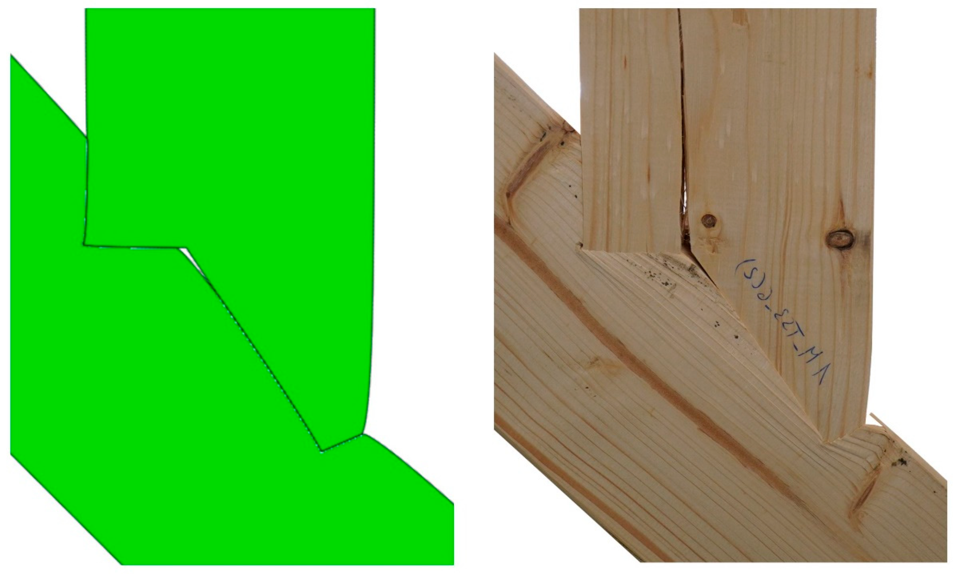
2. Experimental Investigations
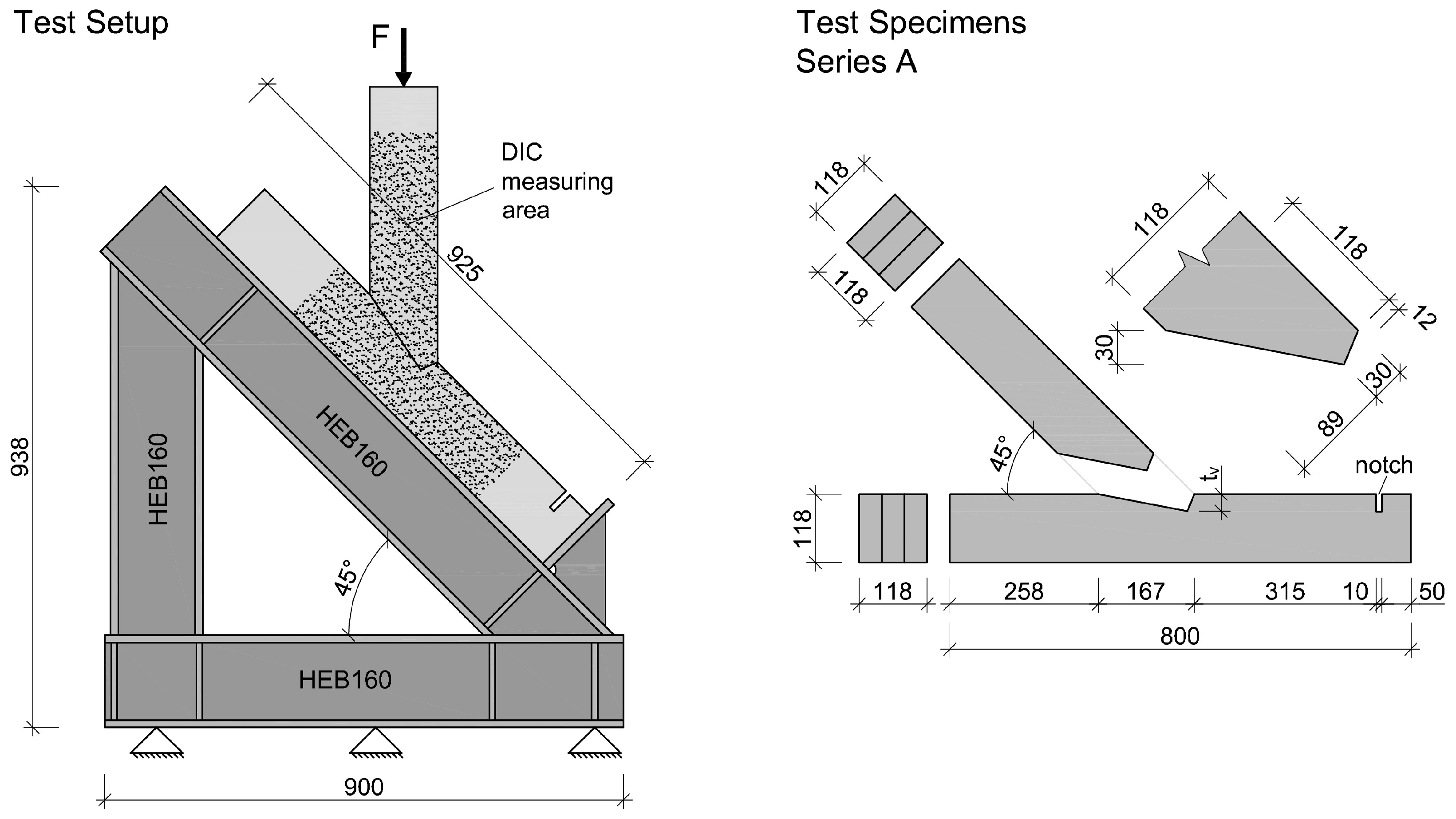
2.1. Test Setup and Test Specimens
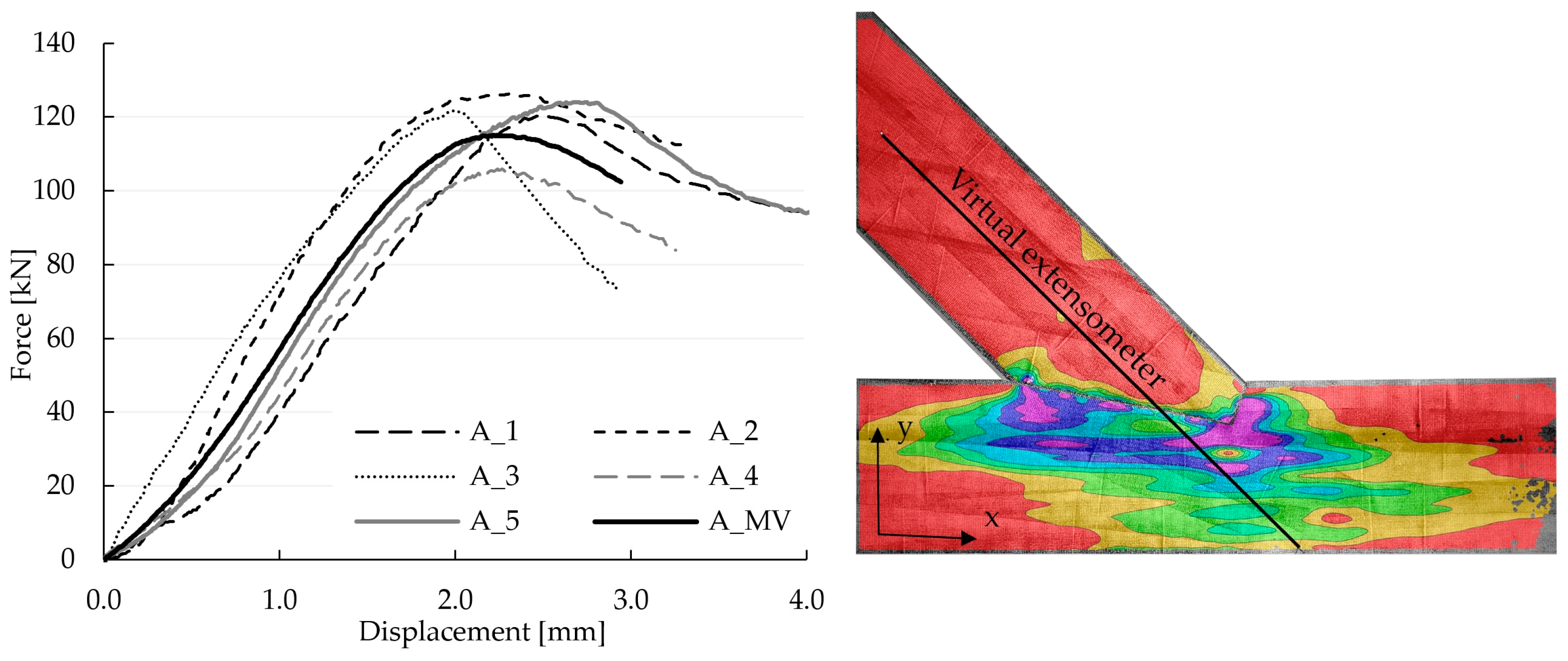
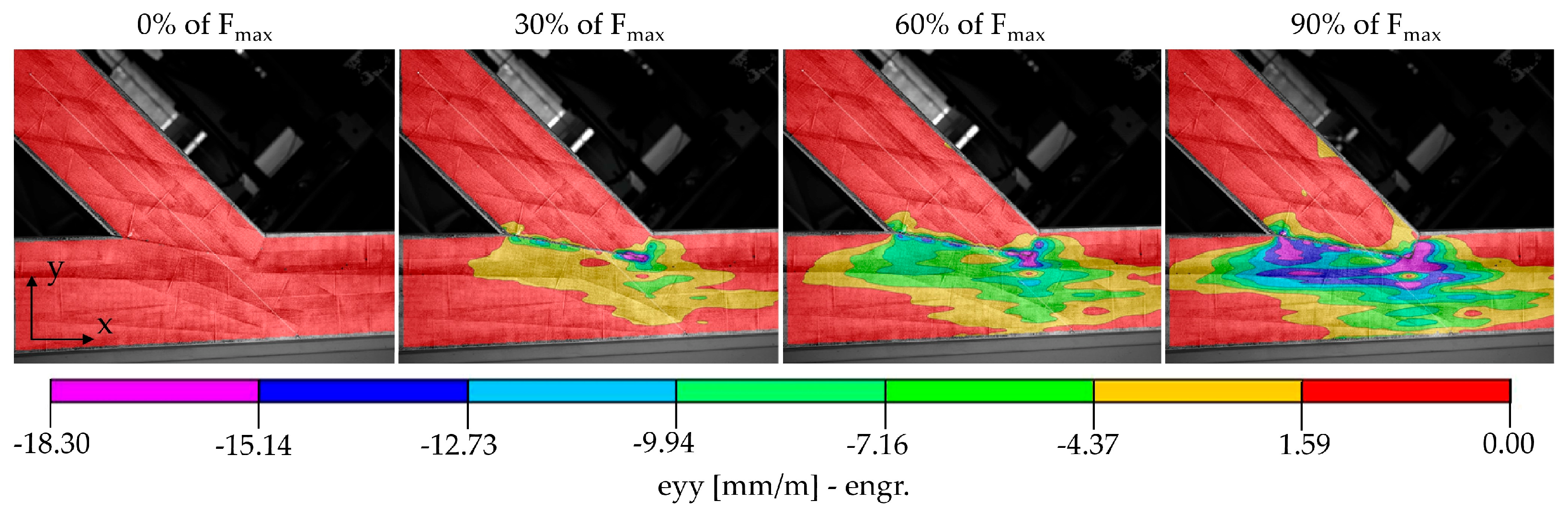
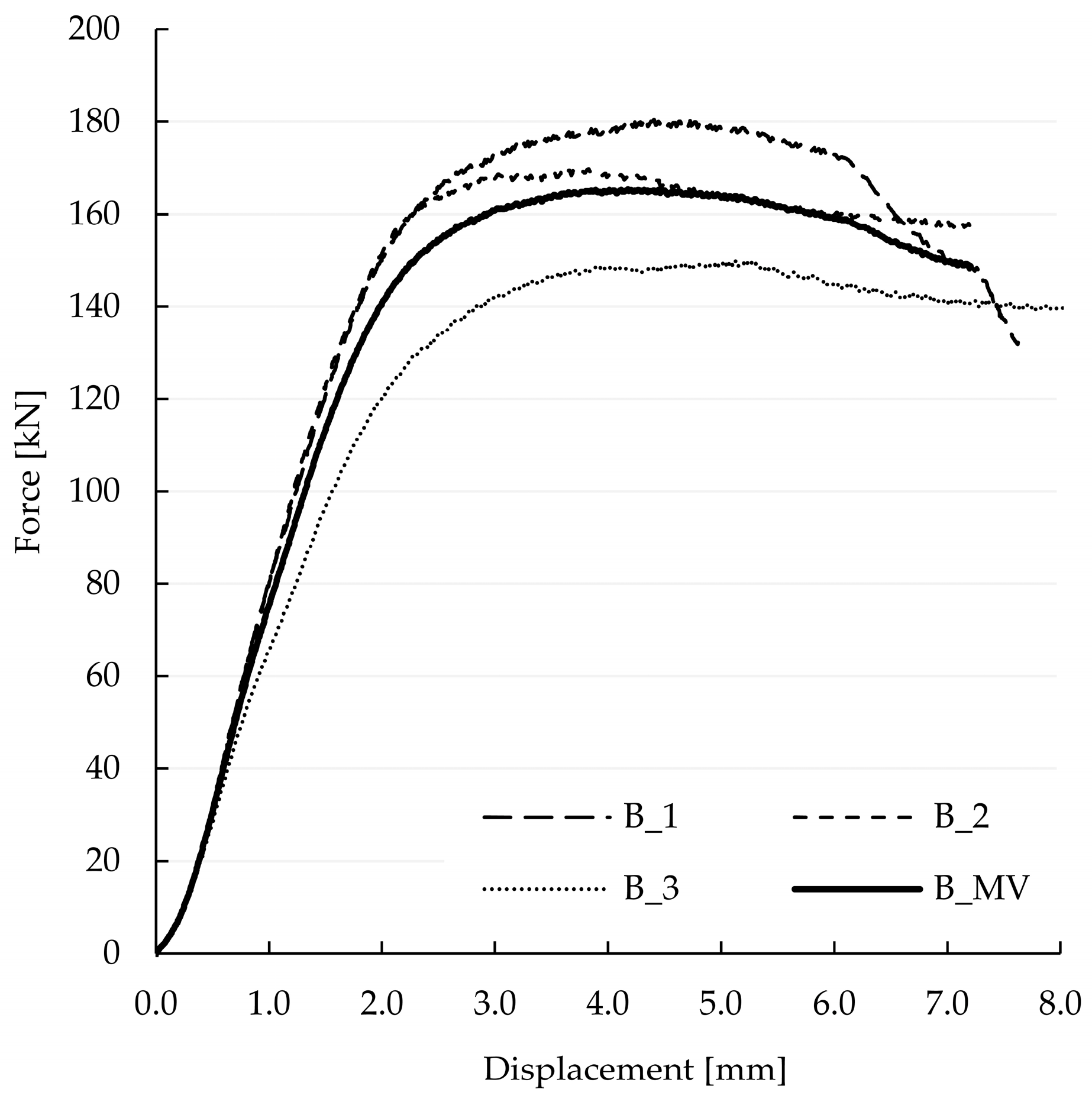
2.2. Results of the Experimental Invesitations
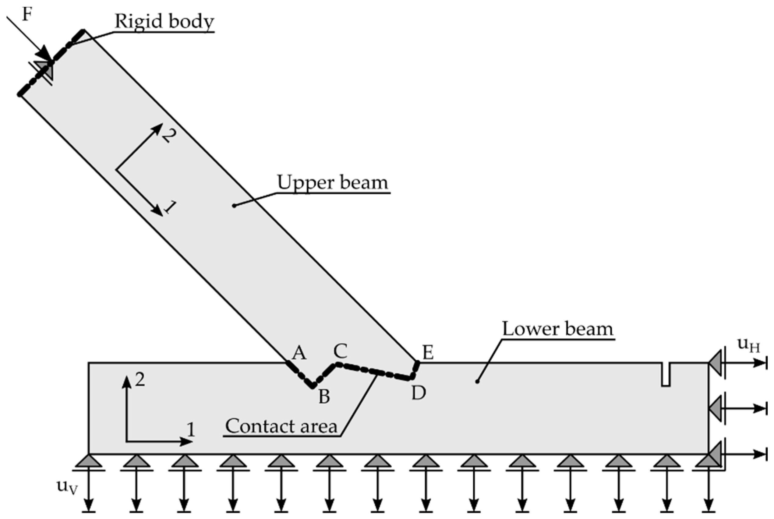
3. Mathematical Model of Timber with the Finite Element Implementation
4. Numerical Calculations
4.1. First Step—Numerical Simulation Using Material Properties According to EN 14080
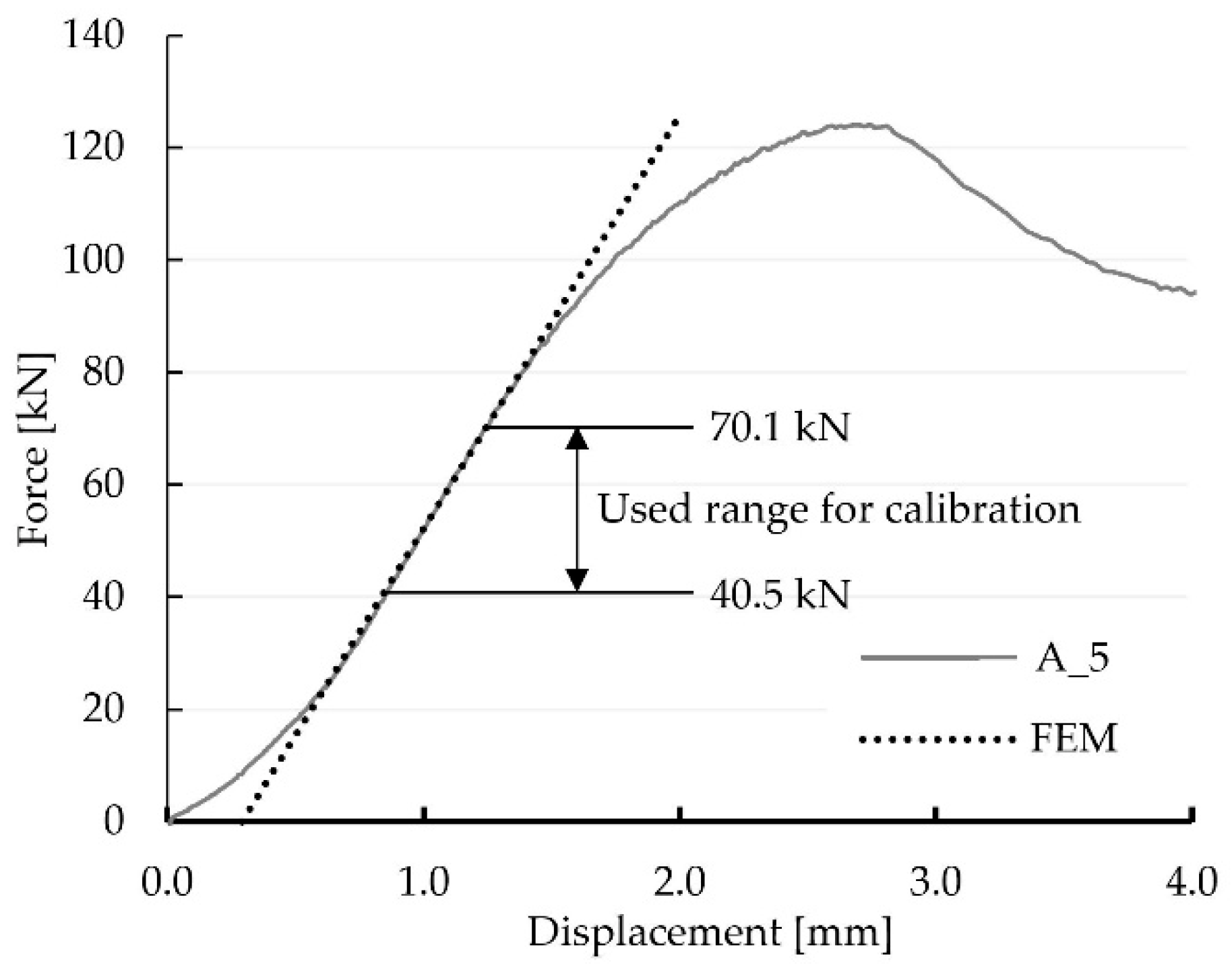
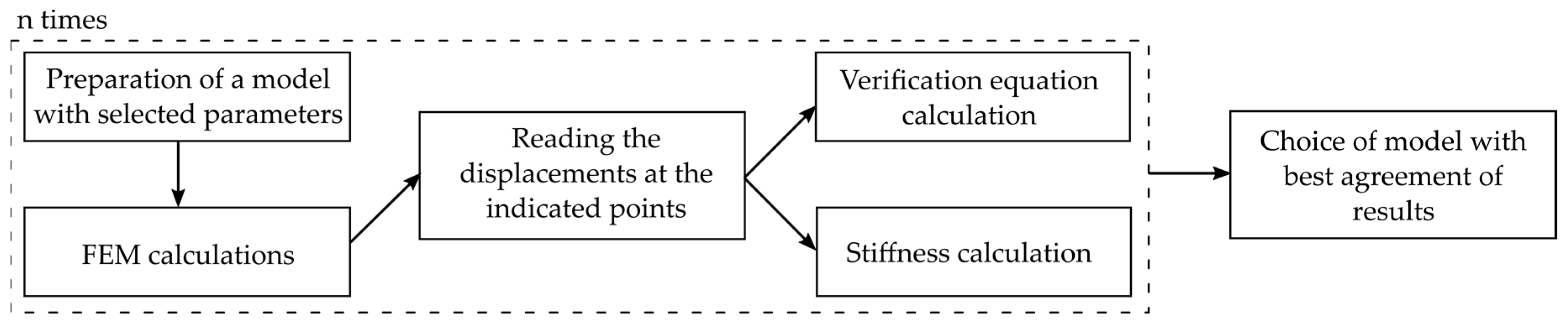
4.2. Calibration of the Numerical Model According to the Results of the Experimental Investiagions
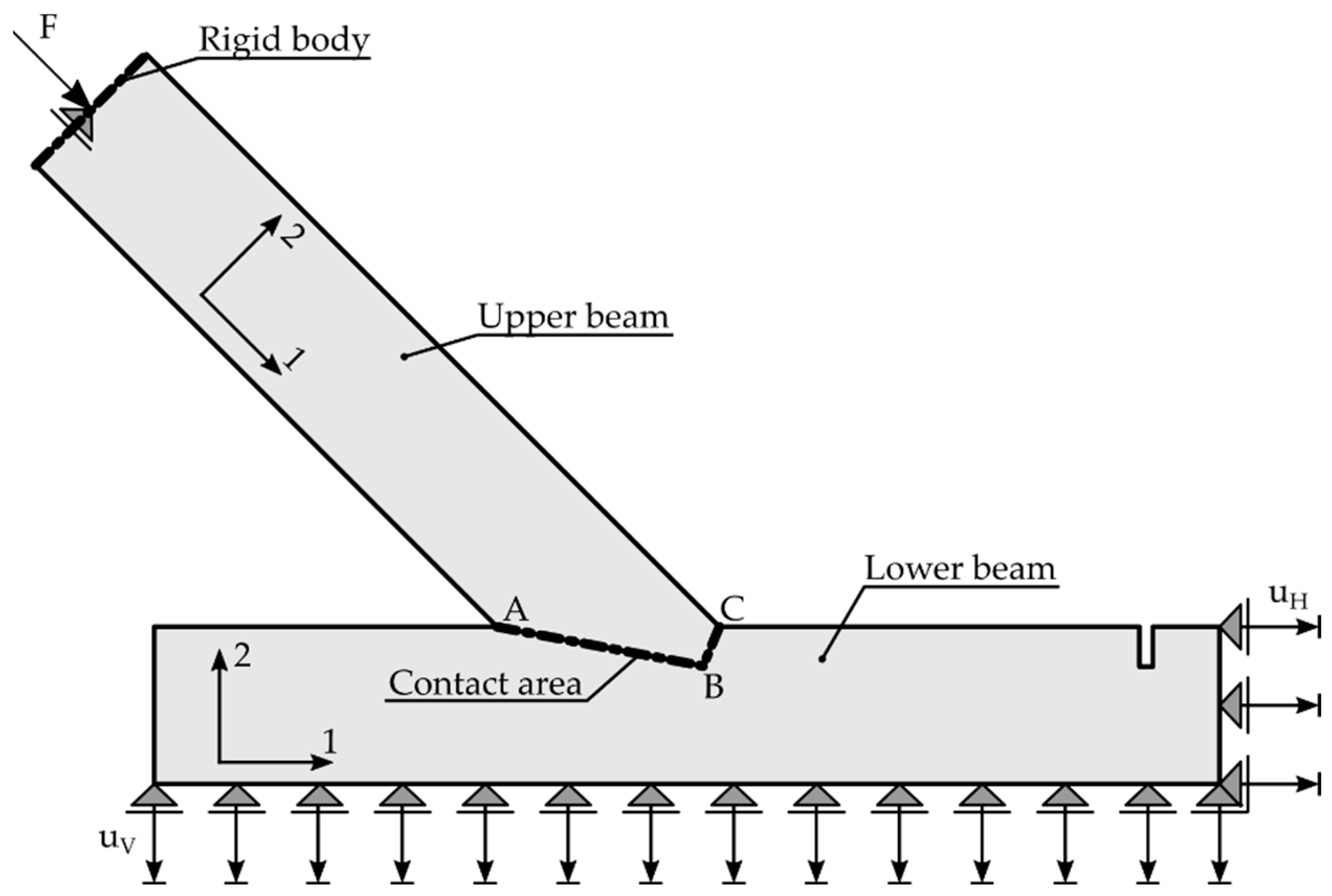
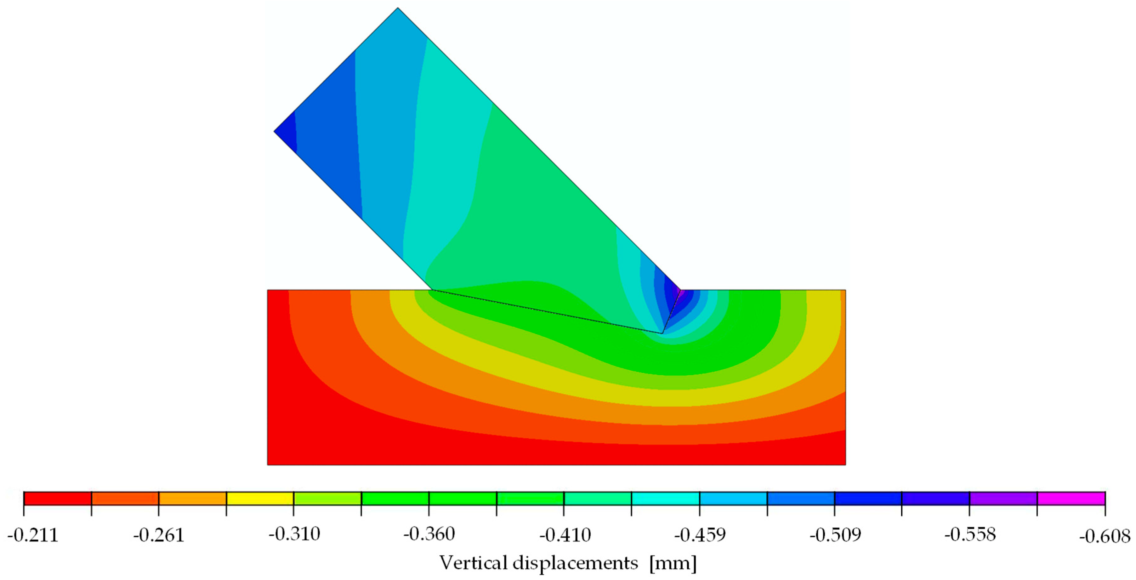
5. Application of the Calibrated Numerical Model on a Double-Step Joint
6. Concluding Remarks
Author Contributions
Funding
Institutional Review Board Statement
Informed Consent Statement
Conflicts of Interest
References
- Anderson, T.R.; Hawkins, E.; Jones, P.D. CO2, the greenhouse effect and global warming: From the pioneering work of Arrhenius and Callendar to today’s Earth System Models. Endeavour 2016, 40, 178–187. [Google Scholar] [CrossRef] [PubMed] [Green Version]
- United Nations Environment Programme. 2019 Global Status Report for Buildings and Construction. 2019. Available online: https://wedocs.unep.org/handle/20.500.11822/30950 (accessed on 6 November 2021).
- Churkina, G.; Organschi, A.; Reyer, C.P.O.; Ruff, A.; Vinke, K.; Liu, Z.; Schellnhuber, H.J. Buildings as a global carbon sink. Nat. Sustain. 2020, 3, 269–276. [Google Scholar] [CrossRef]
- Kromoser, B.; Braun, M. Towards efficiency in constructive timber engineering—Design and optimization of timber trusses. In Proceedings of the IABSE Congress 2019, New York, NY, USA, 4–6 September 2019. [Google Scholar]
- Kromoser, B.; Braun, M. Industrialization of the Design and Production Process of Wooden Trusses. CompWood. 2019. Available online: https://open.lnu.se/index.php/compwood/issue/view/146/Boog%20of%20abstracts (accessed on 10 December 2021).
- Braun, M.; Pantscharowitsch, M.; Kromoser, B. Experimental investigations on the load-bearing behaviour of traditional and newly developed step joints for timber structures. Constr. Build. Mater. 2022, 323, 126557. [Google Scholar] [CrossRef]
- Braun, M.; Kromoser, B. Under Review-The Influence of Inaccuracies in the Production Process on the Load-Bearing Behaviour of Timber Step Joints. SSRN J. 2021. [Google Scholar] [CrossRef]
- CEN. ÖNORM EN 14080: 2013 08 01: Timber Structures—Glued Laminated Timber and Glued Solid Timber—Requirements; European Committee for Standardization: Brussels, Belgium, 2013. [Google Scholar]
- Kandler, G.; Lukacevic, M.; Füssl, J. Experimental study on glued laminated timber beams with well-known knot morphology. Eur. J. Wood Prod. 2018, 76, 1435–1452. [Google Scholar] [CrossRef] [Green Version]
- Fink, G.; Kohler, J. Model for the prediction of the tensile strength and tensile stiffness of knot clusters within structural timber. Eur. J. Wood Prod. 2014, 72, 331–341. [Google Scholar] [CrossRef] [Green Version]
- Vaiana, N.; Sessa, S.; Marmo, F.; Rosati, L. A class of uniaxial phenomenological models for simulating hysteretic phenomena in rate-independent mechanical systems and materials. Nonlinear Dyn. 2018, 93, 1647–1669. [Google Scholar] [CrossRef]
- Vaiana, N.; Sessa, S.; Rosati, L. A generalized class of uniaxial rate-independent models for simulating asymmetric mechanical hysteresis phenomena. Mech. Syst. Signal Process. 2021, 146, 106984. [Google Scholar] [CrossRef]
- Argilaga, A.; Papachristos, E. Bounding the Multi-Scale Domain in Numerical Modelling and Meta-Heuristics Optimization: Application to Poroelastic Media with Damageable Cracks. Materials 2021, 14, 3974. [Google Scholar] [CrossRef]
- Green, A.E.; Zerna, W. Theoretical Elasticity; Courier Corporation: London, UK, 1968. [Google Scholar]
- Thelandersson, S.; Larsen, H.J. (Eds.) Timber Engineering; Wiley: New York, NY, USA, 2003. [Google Scholar]
- Zienkiewicz, O.C.; Taylor, R.L. The Finite Element Method, 5th ed.; Butterworth-Heinemann: Oxford, UK; Boston, MA, USA, 2000. [Google Scholar]
- Mackerle, J. Finite element analyses in wood research: A bibliography. Wood Sci. Technol. 2005, 39, 579–600. [Google Scholar] [CrossRef]
- Villar-García, J.R.; Vidal-López, P.; Crespo, J.; Guaita, M. Analysis of the stress state at the double-step joint in heavy timber structures. Mater. Constr. 2019, 69, 196. [Google Scholar] [CrossRef] [Green Version]
- Al Sabouni-Zawadzka, A.; Gilewski, W.; Pełczyński, J.; Skowronska, M. 3D Finite Element Stress Analysis of Reinforced Double-Tapered Glulam Beams. IOP Conf. Ser. Mater. Sci. Eng. 2019, 661, 012068. [Google Scholar] [CrossRef] [Green Version]
- Gilewski, W.; Pełczyński, J. The Influence of Orthotropy Level for Perpendicular to Grain Stresses in Glulam Double Tapered Beams. 23rd International Conference Engineering Mechanics. 2017. Available online: https://www.engmech.cz/improc/2017/0342.pdf (accessed on 23 October 2021).
- Al Sabouni-Zawadzka, A.; Gilewski, W.; Pełczyński, J. Some considerations on perpendicular to grain stress in double-tapered glulam beams. MATEC Web. Conf. 2017, 117, 00058. [Google Scholar] [CrossRef] [Green Version]
- Al Sabouni-Zawadzka, A.; Gilewski, W.; Pełczyński, J. Perpendicular to grain stress concentrations in glulam beams of irregular shape—Finite element modelling in the context of standard design. Int. Wood Prod. J. 2018, 9, 157–163. [Google Scholar] [CrossRef]
- Abaqus Version 6.13. Simula. ABAQUS User Subroutine Reference Guide; Abaqus: Providence, RI, USA, 2013. [Google Scholar]
- Spaethe, G. Die Sicherheit Tragender Baukonstruktionen; Springer: New York, NY, USA, 1992. [Google Scholar]
- Bedon, C.; Fragiacomo, M. Numerical analysis of timber-to-timber joints and composite beams with inclined self-tapping screws. Compos. Struct. 2019, 207, 13–28. [Google Scholar] [CrossRef]
- Xu, B.-H.; Bouchaïr, A.; Racher, P. Appropriate Wood Constitutive Law for Simulation of Nonlinear Behavior of Timber Joints. J. Mater. Civ. Eng. 2014, 26, 04014004. [Google Scholar] [CrossRef]


| Parameter | Min | Max |
|---|---|---|
| E1 [MPa] | 100 | 12,650 |
| E2 [MPa] | 10 | 400 |
| G12 [MPa] | 50 | 1000 |
| [-] | 0.0 | 0.4 |
| Stress | Value for 30 kN [MPa] | Strength [MPa] | Limit Load [kN] | Location: Point (Beam) | Figure | |
|---|---|---|---|---|---|---|
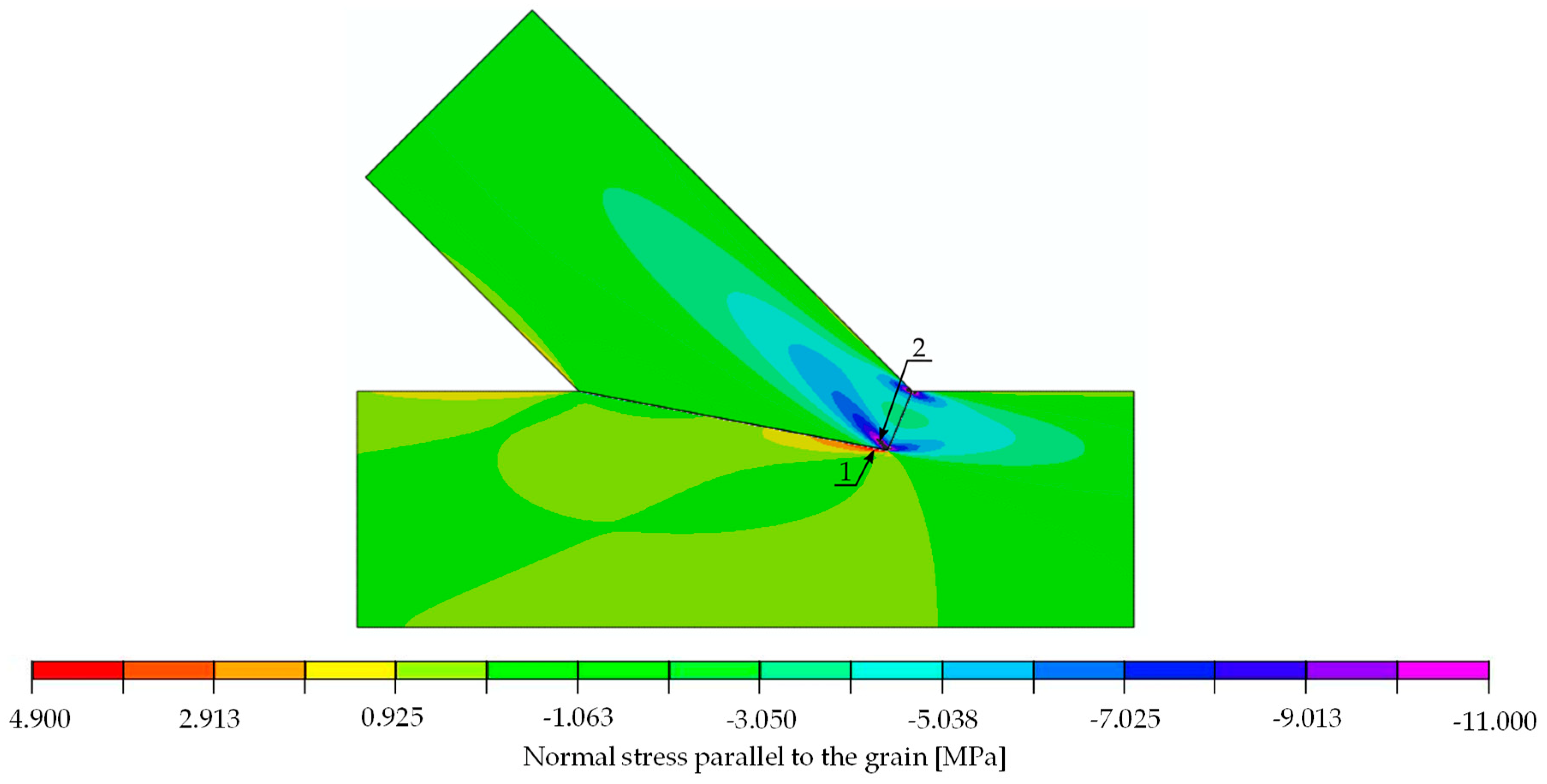
| parallel to the grain | tension | 4.900 | 30.00 | 183.7 | 1 (lower) | Figure 14 |
| compression | 11.000 | 32.00 | 87.3 | 2 (upper) | Figure 14 | |
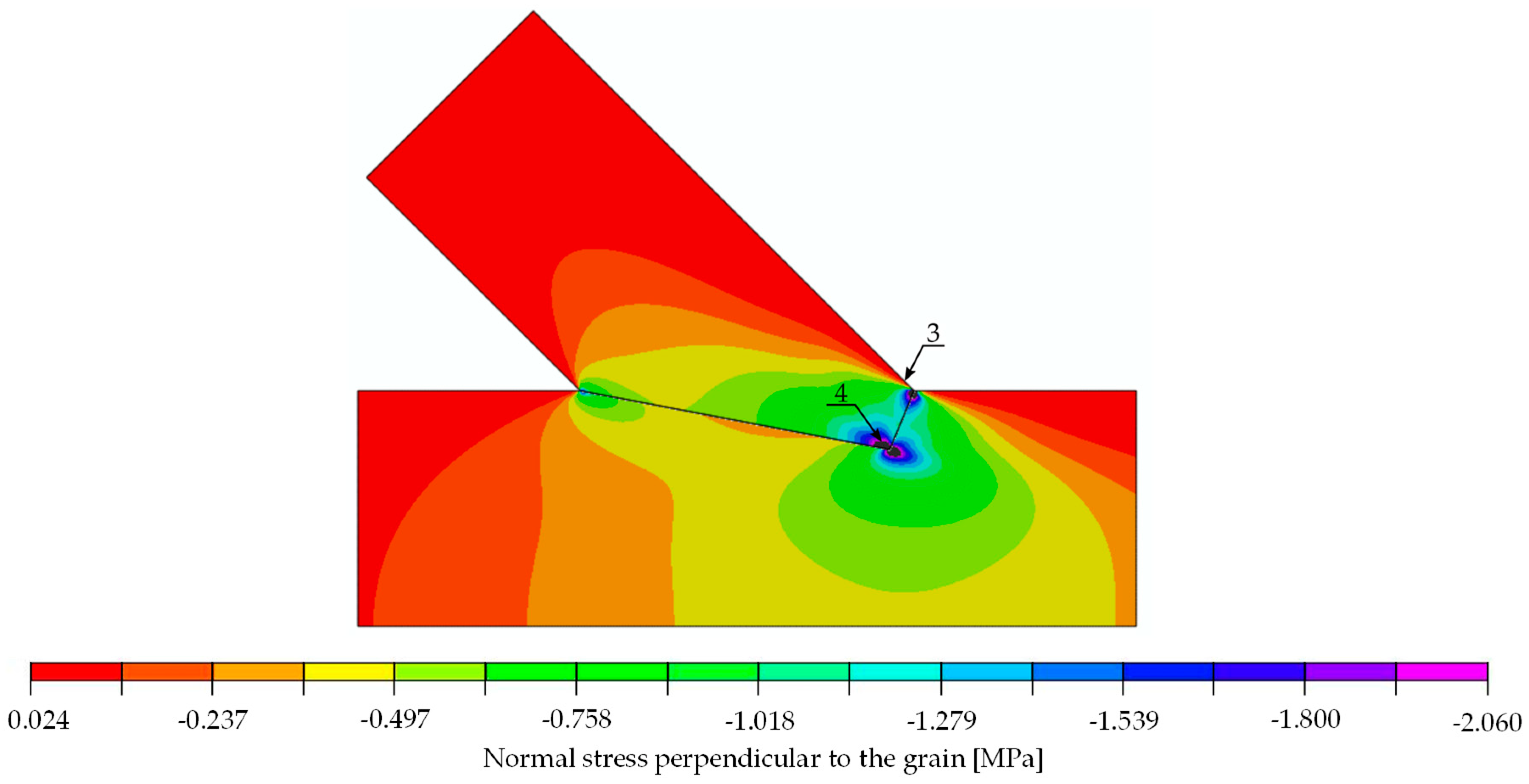
| perpendicular to the grain | tension | 0.024 | 0.50 | 625.0 | 3 (upper) | Figure 15 |
| compression | 2.060 | 3.57 | 52.0 | 4 (upper) | Figure 15 | |
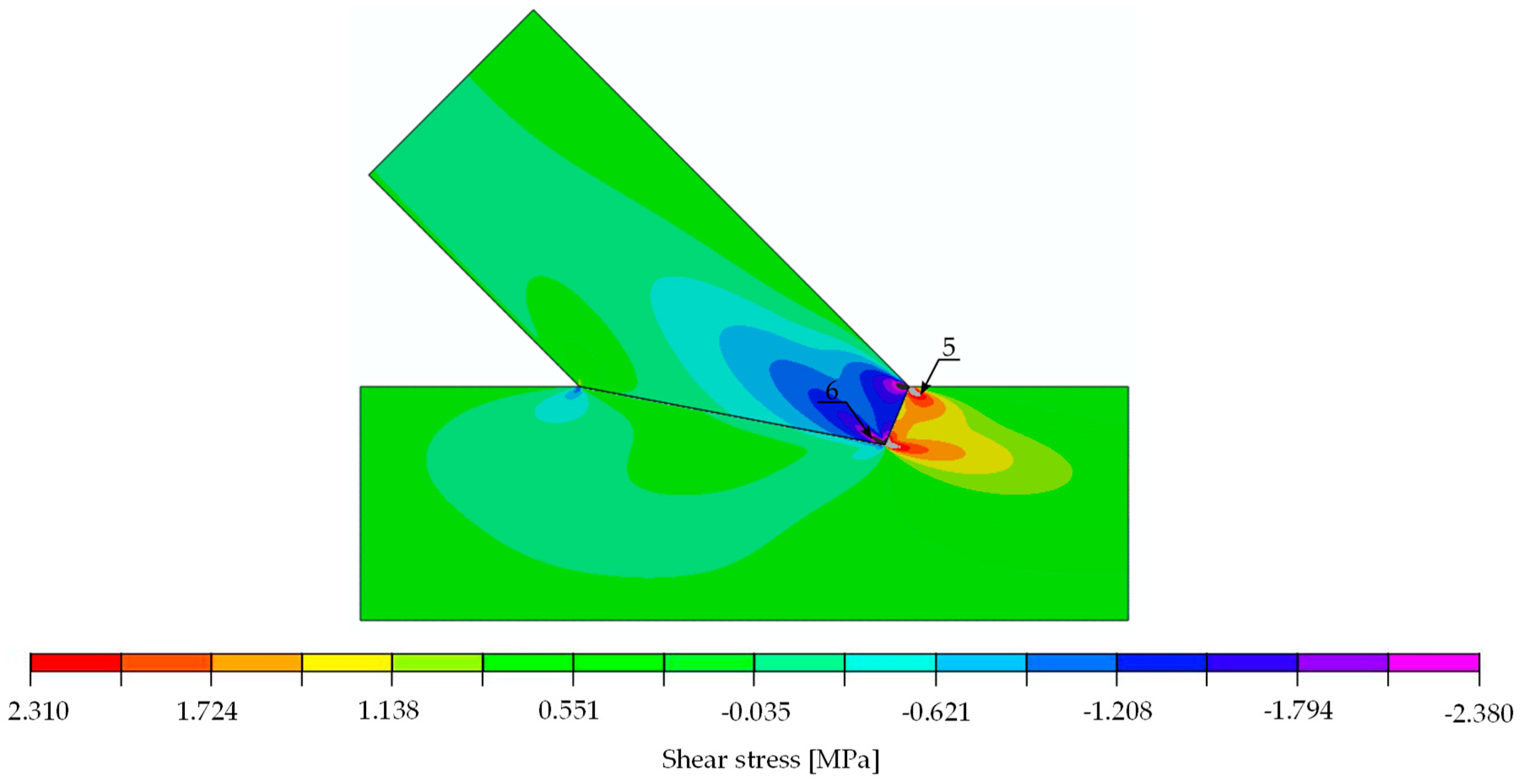
| shear | positive | 2.310 | 3.85 | 50.0 | 5 (lower) | Figure 16 |
| negative | 2.380 | 3.85 | 48.5 | 6 (upper) | Figure 16 | |
| Stress | Value for 29.6 kN [MPa] | Strength [MPa] | Limit Load [kN] | Location: Point (Beam) | Figure | |
|---|---|---|---|---|---|---|
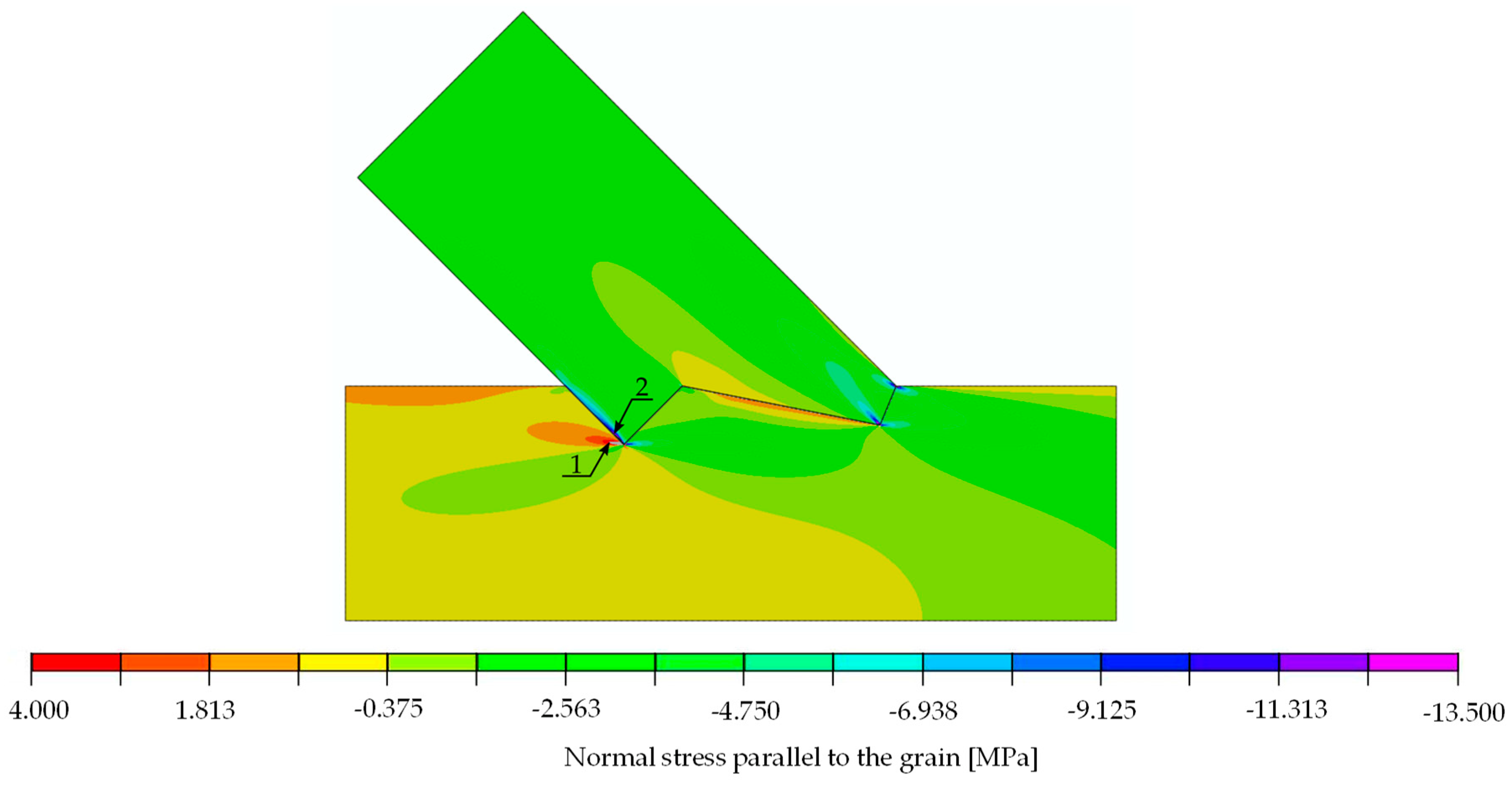
| parallel to the grain | tension | 4.00 | 30.00 | 225.0 | 1 (lower) | Figure 20 |
| compression | 13.49 | 32.00 | 71.2 | 2 (upper) | Figure 20 | |
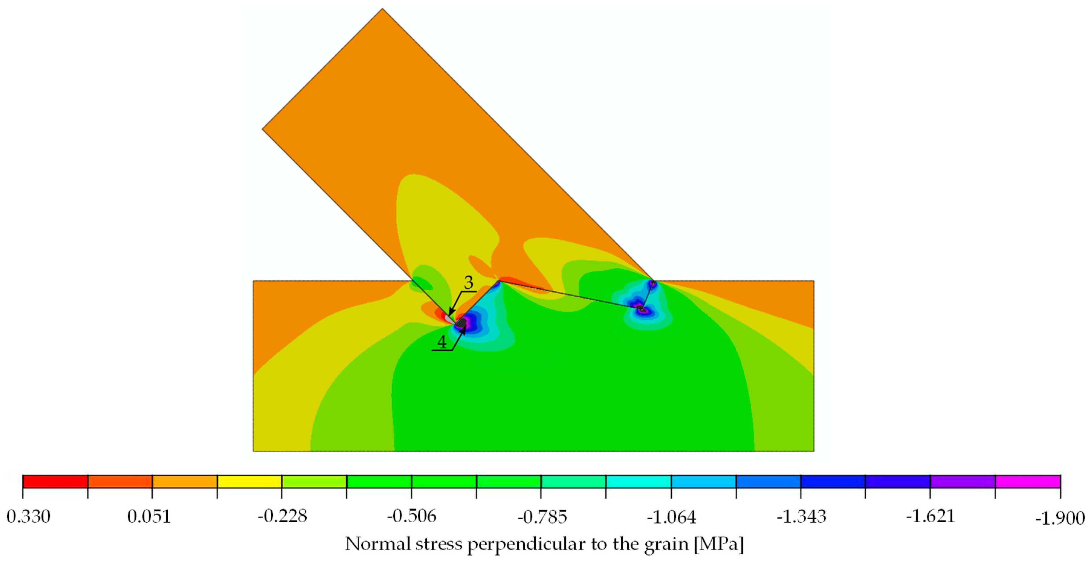
| perpendicular to the grain | tension | 0.33 | 0.50 | 45.5 | 3 (lower) | Figure 21 |
| compression | 1.86 | 3.57 | 57.6 | 4 (lower) | Figure 21 | |
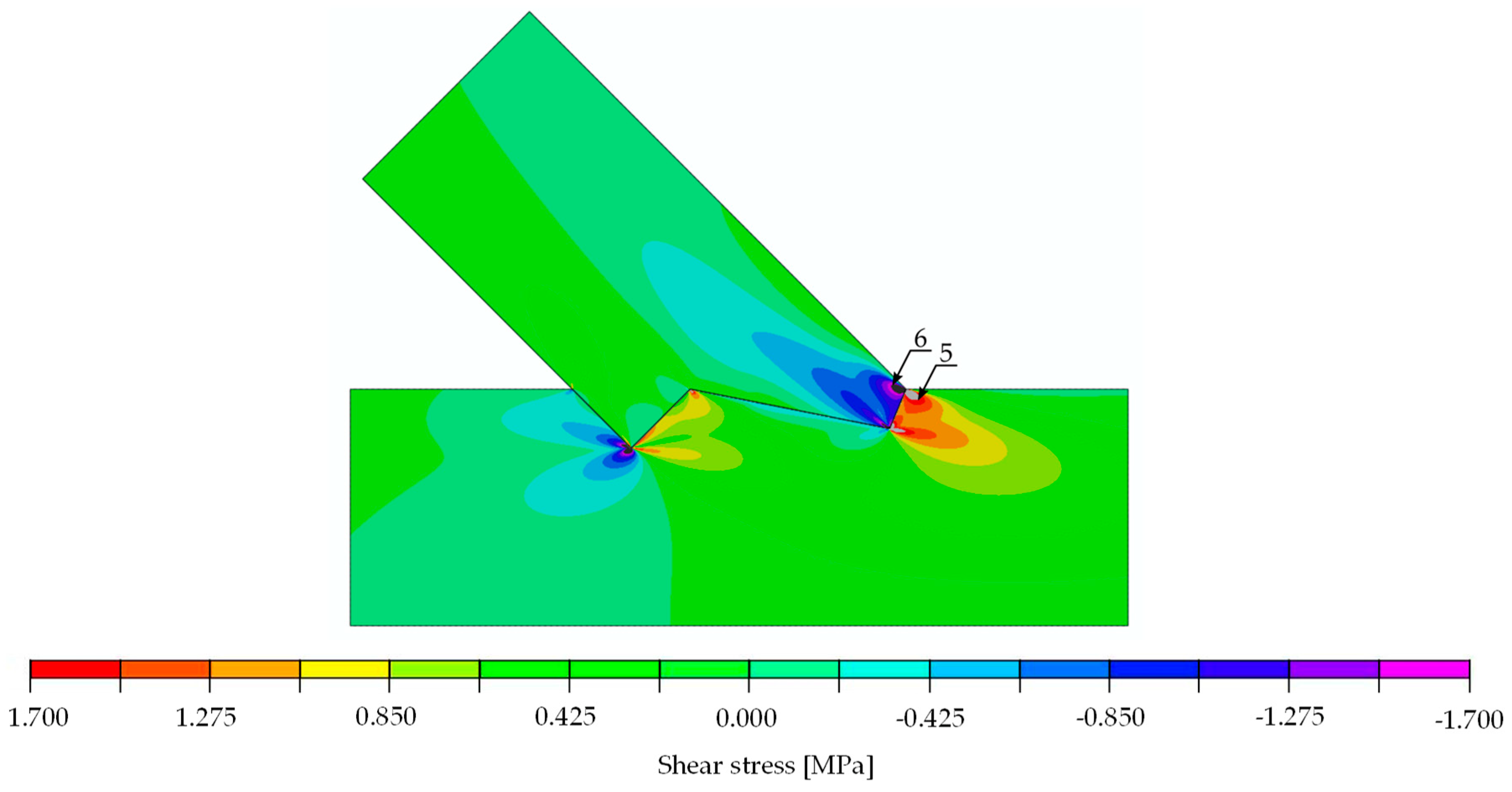
| shear | positive | 1.73 | 3.85 | 66.8 | 5 (lower) | Figure 22 |
| negative | 1.71 | 3.85 | 67.5 | 6 (upper) | Figure 22 | |
Publisher’s Note: MDPI stays neutral with regard to jurisdictional claims in published maps and institutional affiliations. |
© 2022 by the authors. Licensee MDPI, Basel, Switzerland. This article is an open access article distributed under the terms and conditions of the Creative Commons Attribution (CC BY) license (https://creativecommons.org/licenses/by/4.0/).
Share and Cite
Braun, M.; Pełczyński, J.; Al Sabouni-Zawadzka, A.; Kromoser, B. Calibration and Validation of a Linear-Elastic Numerical Model for Timber Step Joints Based on the Results of Experimental Investigations. Materials 2022, 15, 1639. https://doi.org/10.3390/ma15051639
Braun M, Pełczyński J, Al Sabouni-Zawadzka A, Kromoser B. Calibration and Validation of a Linear-Elastic Numerical Model for Timber Step Joints Based on the Results of Experimental Investigations. Materials. 2022; 15(5):1639. https://doi.org/10.3390/ma15051639
Chicago/Turabian StyleBraun, Matthias, Jan Pełczyński, Anna Al Sabouni-Zawadzka, and Benjamin Kromoser. 2022. "Calibration and Validation of a Linear-Elastic Numerical Model for Timber Step Joints Based on the Results of Experimental Investigations" Materials 15, no. 5: 1639. https://doi.org/10.3390/ma15051639
APA StyleBraun, M., Pełczyński, J., Al Sabouni-Zawadzka, A., & Kromoser, B. (2022). Calibration and Validation of a Linear-Elastic Numerical Model for Timber Step Joints Based on the Results of Experimental Investigations. Materials, 15(5), 1639. https://doi.org/10.3390/ma15051639