
Neural Network-Based Multi-Objective Optimization of Adjustable Drawbead Movement for Deep Drawing of Tailor-Welded Blanks


Abstract
:1. Introduction
- It uses non-dominated sorting techniques to provide as close to the Pareto-optimal solution as possible.
- It searches for all non-dominated solutions (F1) considering the crowding distance, which helps obtain diverse results.
- It also uses elitist techniques to preserve the best solution for the current population in the next generation [31].
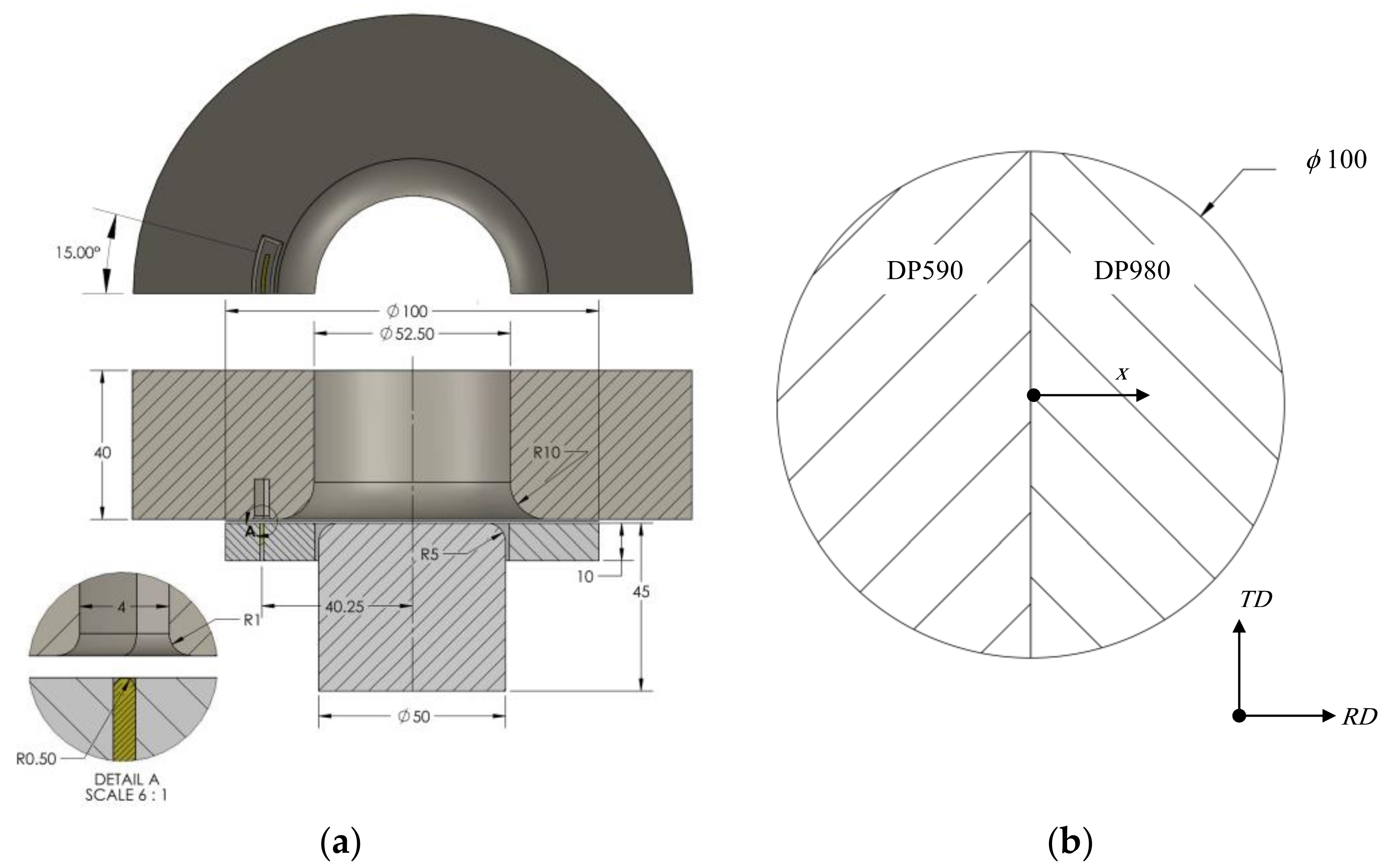
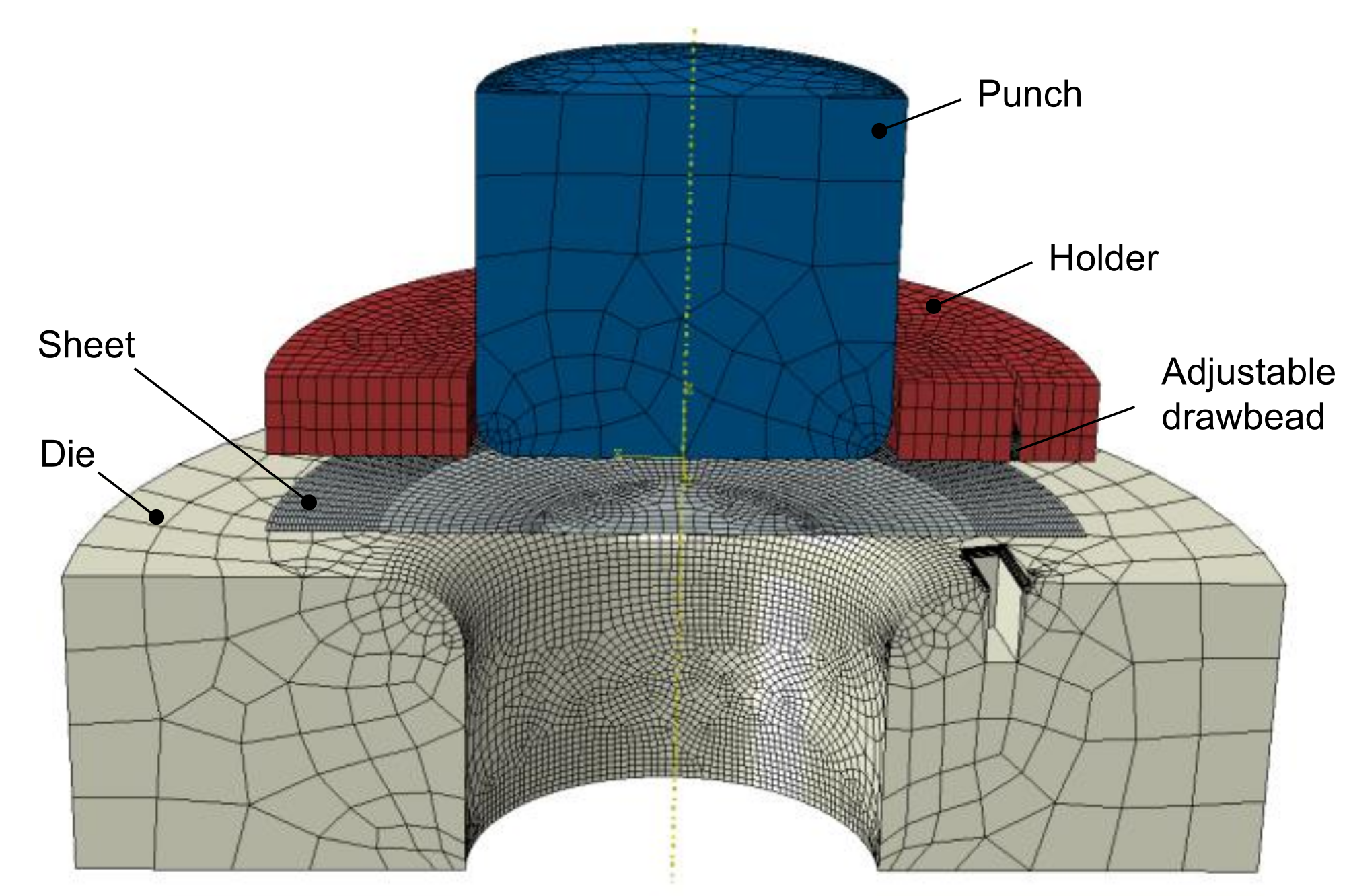
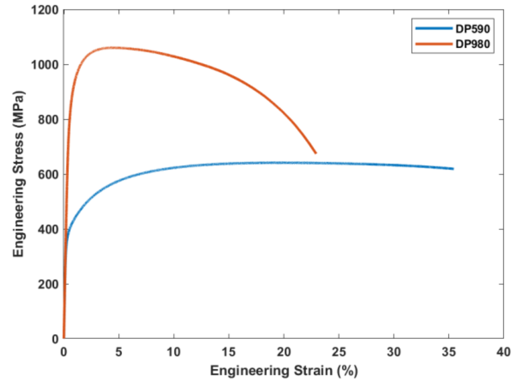
2. Deep Drawing Process of Tailor-Welded Blanks
3. Multi-Objective Optimization
3.1. Objective Functions
3.1.1. Fracture
3.1.2. Centerline Deviation
3.2. Multi-Objective Optimization Algorithm
Fast Non-Dominated Sorting Genetic Algorithm (NSGA-II) for Multi-Objective Problems
- Step 1:
- Population initialization ().
- Step 2:
- Generate a new population (offspring ) by applying crossover and mutation to the current population.
- Step 3:
- Combine two populations (individual and offspring) .
- Step 4:
- Rank the fitness of the new population by employing the non-dominated sorting algorithm and then ordering them as non-dominated fronts , , …, in [42].
- Step 5:
- Calculate the crowding distance.
- Step 6:
- Create a new population () considering rank and crowding distance. When two solutions are in the equivalent rank, the solution with a greater crowding distance is selected.
- Step 7:
- Create offspring population by applying crossover and mutation to .
- Step 8:
- Set and go to Step 2.
3.3. Design of Experiments
3.3.1. RSM
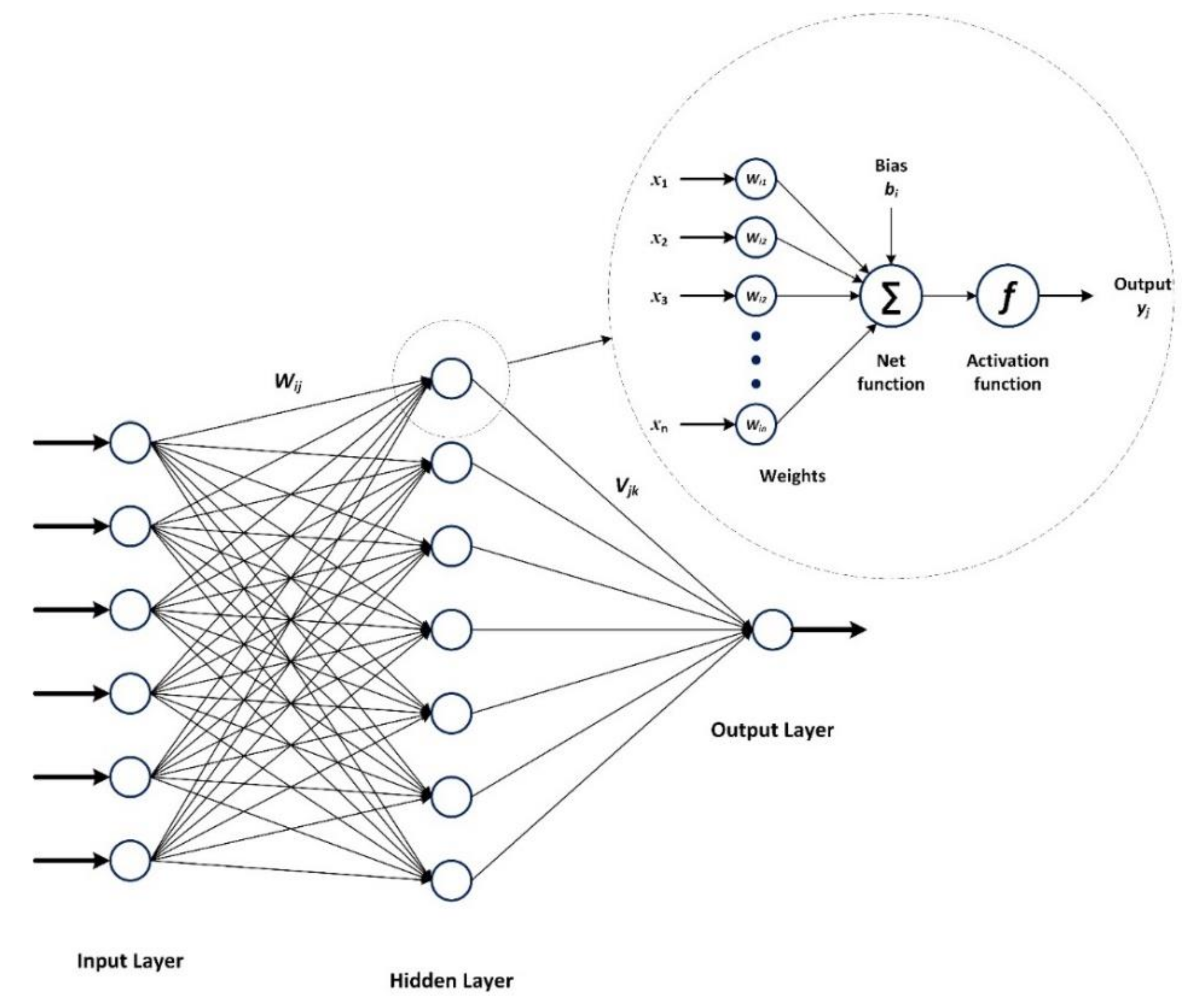
3.3.2. ANN
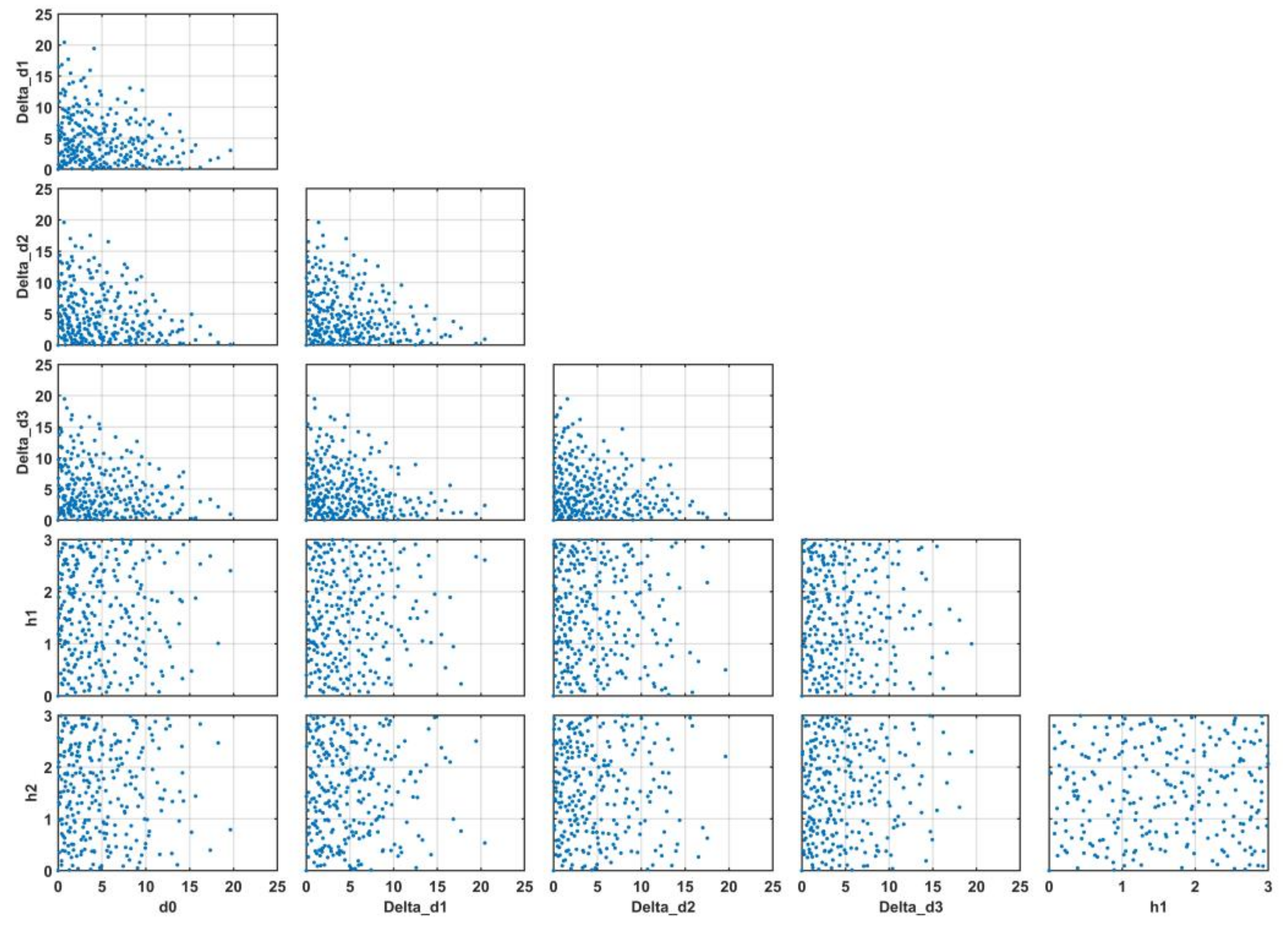
3.3.3. Sobol Sequence Design
3.4. Optimization Model
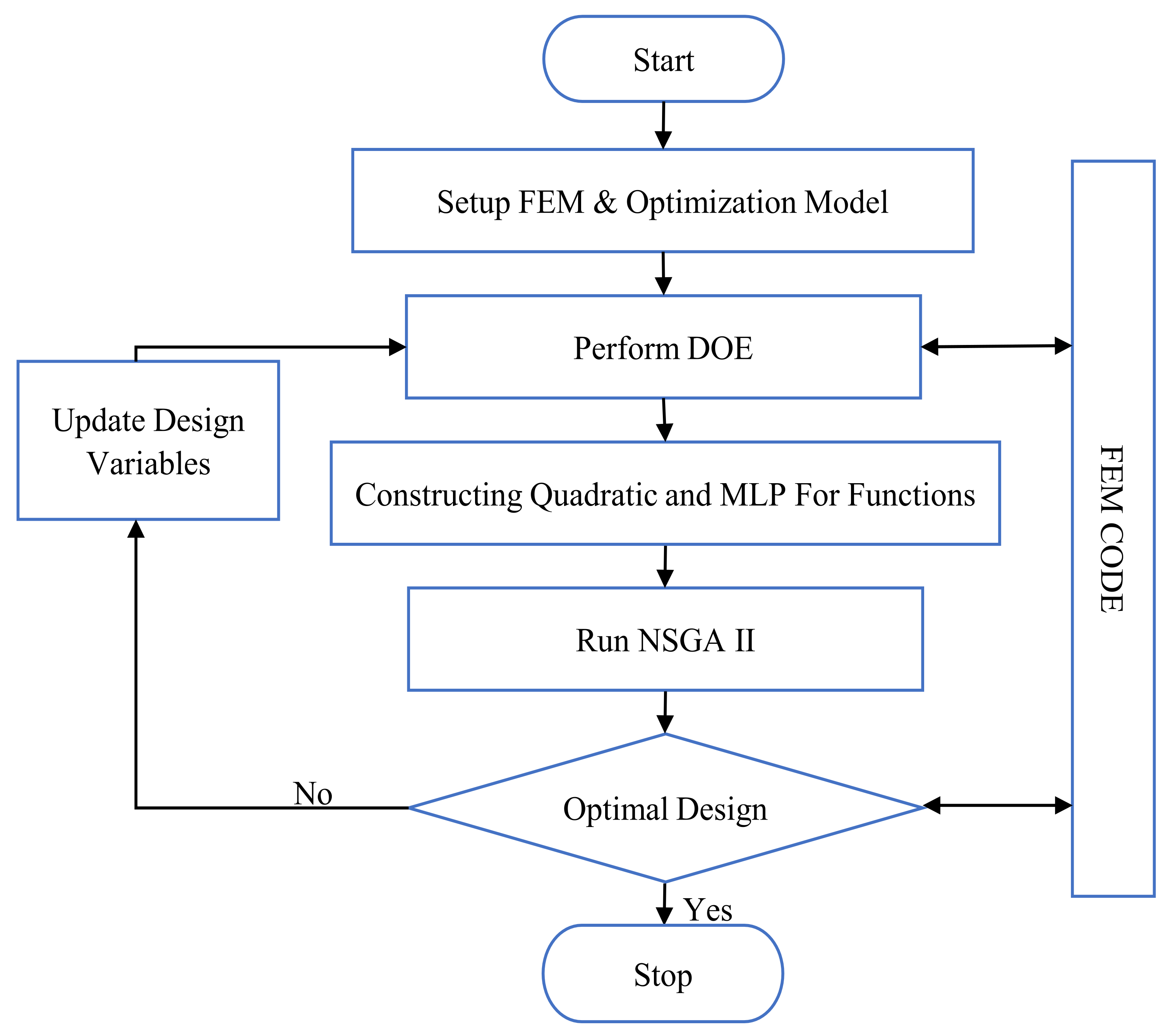
- Step 1:
- The finite element and optimization models were initialized, and subsequent parameters were assigned. (1) Population size P = 250, (2) Reproduction: crossover fraction Fc = 0.8, mutation fraction Fm = 0.1, (3) Stopping criteria: termination generation T = 1000 or stall generations = 200 or function tolerances = 0.00001.
- Step 2:
- To build the RSM and MLP, the objective functions are calculated for each DOE Sobol sequence design observation.
- Step 3:
- According to Equations (7) and (8), the RSM and MLP networks can be created based on the DOE.
- Step 4:
- The NSGA-II algorithm is used to determine the Pareto front. The optimization algorithm uses surrogate models for evaluating the objective function value instead of long-time FEA computation.
- Step 5:
- If the termination criterion is reached, the algorithm is stopped. Otherwise, the process returns to step 3.
4. Results
4.1. RSM and ANN
4.2. Optimization Results
5. Conclusions
- 1.
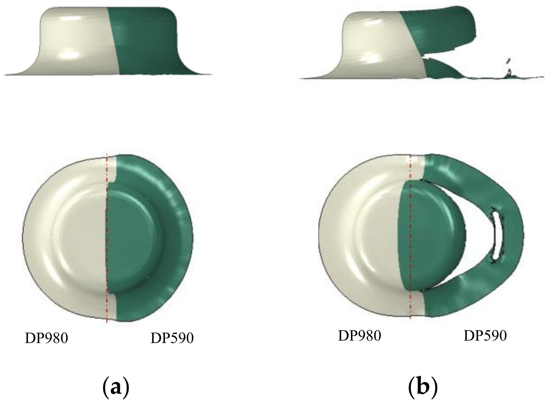
- The proposed procedure successfully determined the optimum movement of the adjustable drawbead to avoid fracture while minimizing the movement of the weld line.
- 2.
- The ANN was more accurate than the RSM in modeling a highly non-linear fracture objective function.
- 3.
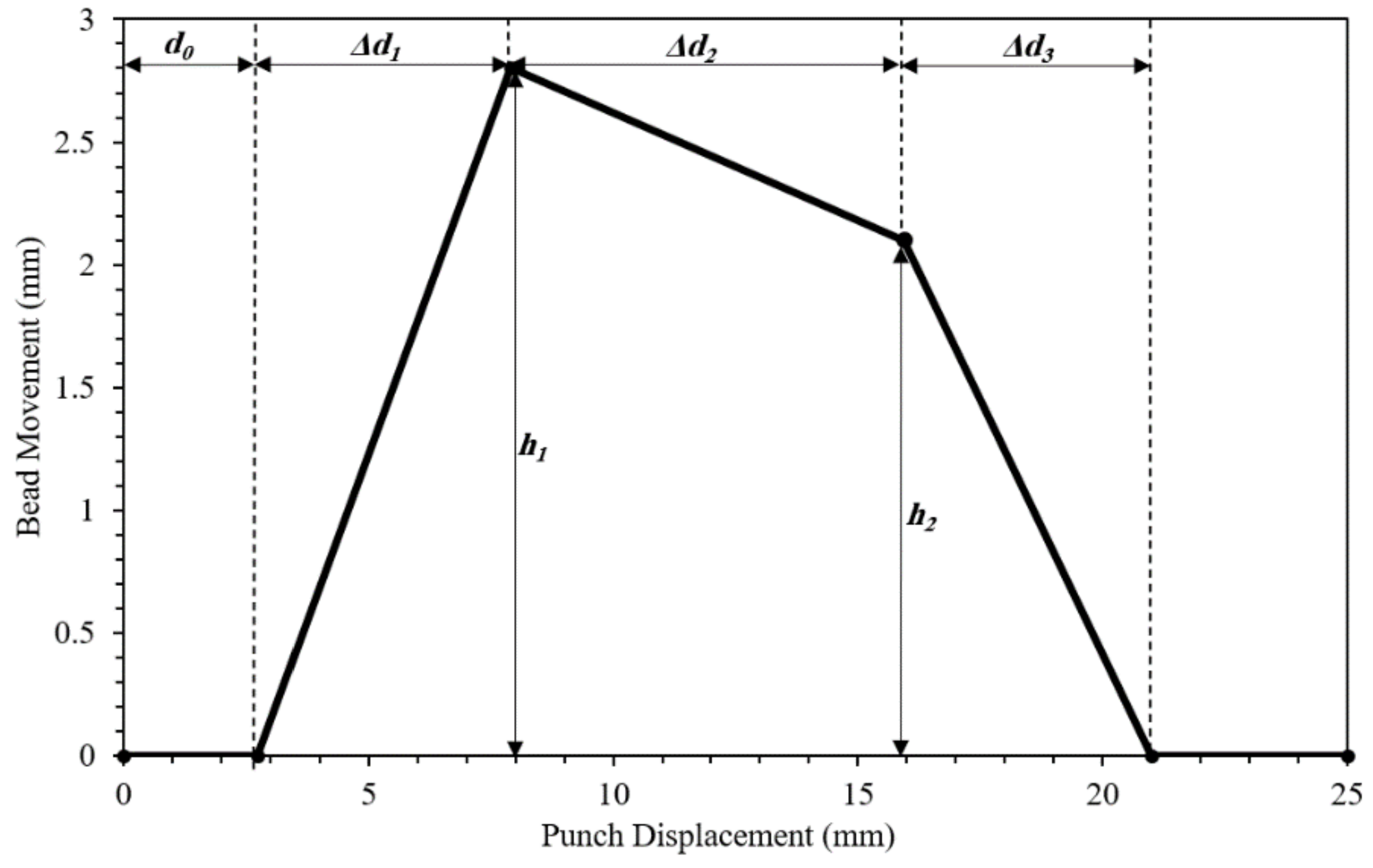
- Among the six design variables of the drawbead movement, the displacement to the initiation of the bead () had the most influence on the fracture and centerline objective functions for both RSM and ANN models.
- 4.
- The design variables of the displacement to the initiation of the bead (), the displacement to the first peak (), and the displacement to the second peak () had a higher effect on centerline deviation than other parameters.
- 5.
- The displacement to the second peak () had the most relative importance in the fracture objective of the ANN, but it had the least importance in the RSM. This difference demonstrates the necessity of using an ANN with high nonlinearity.
- 6.
- A comparison of the optimum case (ANN) and the case with the initially raised bead showed that the delayed initiation of the drawbead is effective in reducing the movement of the weld centerline of the tailor-welded blank.
Author Contributions
Funding
Institutional Review Board Statement
Informed Consent Statement
Data Availability Statement
Conflicts of Interest
References
- Tušek, J.; Kampuš, Z.; Suban, M. Welding of tailored blanks of different materials. J. Mater. Process. Technol. 2001, 119, 180–184. [Google Scholar] [CrossRef]
- Li, J. The Effect of Weld Design on the Formability of Laser Tailor Welded Blanks. Master’s Thesis, University of Waterloo, Waterloo, ON, Canada, 2010. [Google Scholar]
- Rooks, B. Tailor-welded blanks bring multiple benefits to car design. Assem. Autom. 2001, 21, 323–329. [Google Scholar] [CrossRef]
- Chatterjee, S.; Saha, R.; Shome, M.; Ray, R.K. Evaluation of Formability and Mechanical Behavior of Laser-Welded Tailored Blanks Made of Interstitial-Free and Dual-Phase Steels. Met. Mater. Trans. A 2009, 40, 1142–1152. [Google Scholar] [CrossRef]
- Xia, M.; Sreenivasan, N.; Lawson, S.; Zhou, Y.; Tian, Z. A Comparative Study of Formability of Diode Laser Weldments in DP980 and HSLA Steels. J. Eng. Mater. Technol. 2007, 129, 446–452. [Google Scholar] [CrossRef] [Green Version]
- Kinsey, B.; Liu, Z.; Cao, J. A novel forming technology for tailor-welded blanks. J. Mater. Process. Technol. 2000, 99, 145–153. [Google Scholar] [CrossRef]
- Heo, Y.; Choi, Y.; Kim, H.Y.; Seo, D. Characteristics of weld line movements for the deep drawing with drawbeads of tailor-welded blanks. J. Mater. Process. Technol. 2001, 111, 164–169. [Google Scholar] [CrossRef]
- He, S.; Wu, X.; Hu, S.J. Formability enhancement for tailor-welded blanks using blank holding force control. J. Manuf. Sci. Eng. 2003, 125, 461–467. [Google Scholar] [CrossRef]
- Padmanabhan, R.; Oliveira, M.; Menezes, L. Deep drawing of aluminium–steel tailor-welded blanks. Mater. Des. 2008, 29, 154–160. [Google Scholar] [CrossRef]
- Korouyeh, R.S.; Naeini, H.M.; Torkamany, M.; Liaghat, G. Experimental and theoretical investigation of thickness ratio effect on the formability of tailor welded blank. Opt. Laser Technol. 2013, 51, 24–31. [Google Scholar] [CrossRef]
- Hu, X.; Zhao, H.; Xing, Z. Numerical Simulation on Formability of Tailor-Welded Blank with Curved Weld-Line under Different Blank Holder Forces. J. Comput. Theor. Nanosci. 2012, 9, 1236–1241. [Google Scholar] [CrossRef]
- Suresh, V.V.N.S.; Regalla, S.P.; Gupta, A.K. Combined effect of thickness ratio and selective heating on weld line movement in stamped tailor-welded blanks. Mater. Manuf. Process. 2017, 32, 1363–1367. [Google Scholar] [CrossRef]
- Gautam, V.; Kumar, A. Experimental and Numerical Studies on Formability of Tailor Welded Blanks of High Strength Steel. Procedia Manuf. 2019, 29, 472–480. [Google Scholar] [CrossRef]
- Ablat, M.A.; Qattawi, A. Numerical simulation of sheet metal forming: A review. Int. J. Adv. Manuf. Technol. 2016, 89, 1235–1250. [Google Scholar] [CrossRef]
- Kahhal, P.; Yeganehfar, M.; Kashfi, M. An Experimental and Numerical Evaluation of Steel A105 Friction Coefficient Using Different Lubricants at High Temperature. Tribol. Trans. 2021, 65, 25–31. [Google Scholar] [CrossRef]
- Wu, J.; Hovanski, Y.; Miles, M. Investigation of the Thickness Differential on the Formability of Aluminum Tailor Welded Blanks. Metals 2021, 11, 875. [Google Scholar] [CrossRef]
- Heo, Y.M.; Wang, S.H.; Kim, H.Y.; Seo, D.G. The effect of the drawbead dimensions on the weld-line movements in the deep drawing of tailor-welded blanks. J. Mater. Process. Technol. 2001, 113, 686–691. [Google Scholar] [CrossRef]
- Kumar, A.; Digavalli, R.K. Formability prediction of tailor-welded blanks in hydraulic bulging using flow curves from biaxial tensile tests. Proc. Inst. Mech. Eng. Part L J. Mater. Des. Appl. 2021, 235, 853–867. [Google Scholar] [CrossRef]
- Padmanabhan, R.; Oliveira, M.C.; Laurent, H.; Alves, J.L.C.M.; Menezes, L.F. Study on springback in deep drawn tailor welded blanks. Int. J. Mater. Form. 2009, 2, 829–832. [Google Scholar] [CrossRef]
- Aminzadeh, A.; Karganroudi, S.S.; Barka, N. A novel approach of residual stress prediction in ST-14/ST-44 laser welded blanks—Mechanical characterization and experimental validation. Mater. Lett. 2021, 285, 129193. [Google Scholar] [CrossRef]
- Kridli, G.T.; Friedman, P.A.; Sherman, A.M. Formability of Aluminum Tailor-Welded Blanks; SAE 2000-01-0772; SAE International: Warrendale, PA, USA, 2000; pp. 1–9. [Google Scholar]
- Asadian-Ardakani, M.H.; Morovvati, M.R.; Mirnia, M.J.; Dariani, B.M. Theoretical and experimental investigation of deep drawing of tailor-welded IF steel blanks with non-uniform blank holder forces. Proc. Inst. Mech. Eng. Part B J. Eng. Manuf. 2016, 231, 286–300. [Google Scholar] [CrossRef]
- Panda, S.K.; Kumar, D.R.; Kumar, H.; Nath, A. Characterization of tensile properties of tailor welded IF steel sheets and their formability in stretch forming. J. Mater. Process. Technol. 2007, 183, 321–332. [Google Scholar] [CrossRef]
- Lim, Y.; Venugopal, R.; Ulsoy, A.G. Advances in the Control of Sheet Metal Forming. IFAC Proc. Vol. 2008, 41, 1875–1883. [Google Scholar] [CrossRef] [Green Version]
- Li, R.; Weinmann, K.J. Formability in Non-Symmetric Aluminium Panel Drawing Using Active Drawbeads. CIRP Ann. 1999, 48, 209–212. [Google Scholar] [CrossRef]
- Li, R.; Bohn, M.; Weinmann, K.; Chandra, A. A Study of the Optimization of Sheet Metal Drawing with Active Drawbeads. J. Manuf. Process. 2000, 2, 205–216. [Google Scholar] [CrossRef]
- Wang, W.-R.; Chen, G.-L.; Lin, Z.-Q. Application of new VBHF optimization strategy to improve formability of automobile panels with aluminum alloy sheet. Trans. Nonferr. Met. Soc. China 2010, 20, 471–477. [Google Scholar] [CrossRef]
- Dhumal, A.T.; Narayanan, R.G.; Kumar, G.S. Simulation based expert system to predict the deep drawing behaviour of tailor welded blanks. Int. J. Model. Identif. Control 2012, 15, 164. [Google Scholar] [CrossRef]
- Hariharan, K.; Nguyen, N.-T.; Chakraborti, N.; Lee, M.-G.; Barlat, F. Multi-Objective Genetic Algorithm to Optimize Variable Drawbead Geometry for Tailor Welded Blanks Made of Dissimilar Steels. Steel Res. Int. 2014, 85, 1597–1607. [Google Scholar] [CrossRef]
- Williams, B.A.; Cremaschi, S. Surrogate Model Selection for Design Space Approximation and Surrogate based Optimization. Comput. Aided Chem. Eng. 2019, 47, 353–358. [Google Scholar]
- Subashini, G.; Bhuvaneswari, M.C. Comparison of multi-objective evolutionary approaches for task scheduling in distributed computing systems. Sādhanā 2012, 37, 675–694. [Google Scholar] [CrossRef]
- Rahimi, I.; Gandomi, A.H.; Deb, K.; Chen, F.; Nikoo, M.R. Scheduling by NSGA-II: Review and Bibliometric Analysis. Processes 2022, 10, 98. [Google Scholar] [CrossRef]
- POSCO. Automotive Steel. Available online: https://product.posco.com (accessed on 1 December 2021).
- Hur, Y.C.; Kim, D.; Kim, B.M.; Kang, C.Y.; Lee, M.-G.; Kim, J.H. Measurement of Weld Zone Properties of Laser-Welded Tailor-Welded Blanks and Its Application to Deep Drawing. Int. J. Automot. Technol. 2020, 21, 615–622. [Google Scholar] [CrossRef]
- Sun, G.; Li, G.; Gong, Z.; Cui, X.-Y.; Yang, X.; Li, Q. Multiobjective robust optimization method for drawbead design in sheet metal forming. Mater. Des. 2010, 31, 1917–1929. [Google Scholar] [CrossRef]
- Kahhal, P.; Brooghani, S.Y.A.; Azodi, H.D. Multi-objective Optimization of Sheet Metal Forming Die Using Genetic Algorithm Coupled with RSM and FEA. J. Fail. Anal. Prev. 2013, 13, 771–778. [Google Scholar] [CrossRef]
- Hiroyasu, T.; Miki, M.; Kamiura, J.; Watanabe, S.; Hiroyasu, H. Multi-Objective Optimization of Diesel Engine Emissions and Fuel Economy Using Genetic Algorithms and Phenomenological Model; SAE Technical Paper; SAE International: Warrendale, PA, USA, 2002. [Google Scholar]
- Kahhal, P.; Brooghani, S.Y.A.; Azodi, H.D. Multi-objective optimization of sheet metal forming die using FEA coupled with RSM. J. Mech. Sci. Technol. 2013, 27, 3835–3842. [Google Scholar] [CrossRef]
- Deb, K.; Pratap, A.; Agarwal, S.; Meyarivan, T. A fast and elitist multiobjective genetic algorithm: NSGA-II. IEEE Trans. Evol. Comput. 2002, 6, 182–197. [Google Scholar] [CrossRef] [Green Version]
- Konak, A.; Coit, D.W.; Smith, A.E. Multi-objective optimization using genetic algorithms: A tutorial. Reliab. Eng. Syst. Saf. 2006, 91, 992–1007. [Google Scholar] [CrossRef]
- Goldberg, D. Genetic Algorithms in Search, Optimization and Machine Learning; Addsion-Wesley Longman: Boston, MA, USA, 1989. [Google Scholar]
- Ram, D.S.H.; Bhuvaneswari, M.C.; Prabhu, S.S. A Novel Framework for Applying Multiobjective GA and PSO Based Approaches for Simultaneous Area, Delay, and Power Optimization in High Level Synthesis of Datapaths. VLSI Des. 2012, 2012, 273276. [Google Scholar]
- Deb, K. Multi-Objective Optimization Using Evolutionary Algorithms; John Wiley & Sons, Inc.: Hoboken, NJ, USA, 2001. [Google Scholar]
- Jansson, T.; Nilsson, L.; Redhe, M. Using surrogate models and response surfaces in structural optimization–with application to crashworthiness design and sheet metal forming. Struct. Multidiscip. Optim. 2003, 25, 129–140. [Google Scholar] [CrossRef]
- Khalili, K.; Shahri, S.E.E.; Kahhal, P.; Khalili, M.S. Wrinkling Study in Tube Hydroforming Process. Key Eng. Mater. 2011, 473, 151–158. [Google Scholar] [CrossRef]
- Biglin, M. Isobaric vapour–liquid equilibrium calculations of binary. J. Serb. Chem. Soc. 2004, 69, 669–674. [Google Scholar]
- Sobol’, I. On the distribution of points in a cube and the approximate evaluation of integrals. USSR Comput. Math. Math. Phys. 1967, 7, 86–112. [Google Scholar] [CrossRef]


| Material | C | Mn | Si | P | S |
|---|---|---|---|---|---|
| DP590 | 0.1 | 2 | 0.2 | 0.03 | 0.003 |
| DP980 | 0.1 | 2.6 | 0.3 | 0.03 | 0.003 |
| Material | DP590 | DP980 |
|---|---|---|
| Thickness, mm | 1.0 | 1.0 |
| Young’s modulus, GPa | 210 | 210 |
| Poisson’s ratio | 0.3 | 0.3 |
| Yield strength, MPa | 382 | 849 |
| Tensile strength, MPa | 643 | 1058 |
| Objective | Fracture | Centerline Deviation |
|---|---|---|
| Neurons in the input layer | 3 | 3 |
| Number of hidden layers | 1 | 1 |
| Neurons in the hidden layer | 9 | 8 |
| Neurons in the output layer | 1 | 1 |
| Training algorithm | Levenberg–Marquardt Back-Propagation | Levenberg–Marquardt Back-Propagation |
| Activation function (Hidden Layer) | Tansig | Tansig |
| Activation function (Output Layer) | Purelin | Purelin |
| Validation data fraction (%) | 15 | 15 |
| Test data fraction (%) | 15 | 15 |
| Objective | Model | MSE | RMSE | R |
|---|---|---|---|---|
| Fracture | RSM | 4.3437 × 10⁻⁸ | 2.08414 × 10⁻⁴ | 0.883 |
| Fracture | ANN | 1.30063 × 10⁻⁸ | 1.14045 × 10⁻⁴ | 0.967 |
| Centerline | RSM | 9.86692 × 10⁻³ | 4.32202 × 10⁻² | 0.978 |
| Centerline | ANN | 4.32203 × 10⁻² | 9.93323 × 10⁻² | 0.996 |
| Variable/Objective | No Bead | Fixed Bead | ANN Optimum (Initially Raised Bead) | RSM Optimum | ANN Optimum |
|---|---|---|---|---|---|
| d0 (mm) | 0 | 0 | 0 | 1.566289 | 0.470124 |
| Δd1 (mm) | 0 | 0 | 0 | 0.538199 | 0.466919 |
| Δd2 (mm) | 0 | 25 | 3.921509 | 4.233494 | 3.921509 |
| Δd3 (mm) | 0 | 0 | 4.959106 | 5.225806 | 4.959106 |
| h1 (mm) | 0 | 3 | 2.833374 | 2.923667 | 2.833374 |
| h2 (mm) | 0 | 3 | 2.695679 | 1.711225 | 2.695679 |
| Fracture (predicted) | −0.060388 | 19.77237 | 0.2432341 | −0.00015 | 0.20930 |
| Fracture (FE) | 0 | 0.003269 | 0 | 0 | 0 |
| Centerline (predicted) | 1.3041367 | −0.256515 | −0.043089 | −0.06106 | −0.06766 |
| Centerline (FE) | 1.3015800 | −0.141269 | 0.159516 | 0.064793 | 0.00076 |
Publisher’s Note: MDPI stays neutral with regard to jurisdictional claims in published maps and institutional affiliations. |
© 2022 by the authors. Licensee MDPI, Basel, Switzerland. This article is an open access article distributed under the terms and conditions of the Creative Commons Attribution (CC BY) license (https://creativecommons.org/licenses/by/4.0/).
Share and Cite
Kahhal, P.; Jung, J.; Hur, Y.C.; Moon, Y.H.; Kim, J.H. Neural Network-Based Multi-Objective Optimization of Adjustable Drawbead Movement for Deep Drawing of Tailor-Welded Blanks. Materials 2022, 15, 1430. https://doi.org/10.3390/ma15041430
Kahhal P, Jung J, Hur YC, Moon YH, Kim JH. Neural Network-Based Multi-Objective Optimization of Adjustable Drawbead Movement for Deep Drawing of Tailor-Welded Blanks. Materials. 2022; 15(4):1430. https://doi.org/10.3390/ma15041430
Chicago/Turabian StyleKahhal, Parviz, Jaebong Jung, Yong Chan Hur, Young Hoon Moon, and Ji Hoon Kim. 2022. "Neural Network-Based Multi-Objective Optimization of Adjustable Drawbead Movement for Deep Drawing of Tailor-Welded Blanks" Materials 15, no. 4: 1430. https://doi.org/10.3390/ma15041430
APA StyleKahhal, P., Jung, J., Hur, Y. C., Moon, Y. H., & Kim, J. H. (2022). Neural Network-Based Multi-Objective Optimization of Adjustable Drawbead Movement for Deep Drawing of Tailor-Welded Blanks. Materials, 15(4), 1430. https://doi.org/10.3390/ma15041430