
Rice-Husk Shredding as a Means of Increasing the Long-Term Mechanical Properties of Earthen Mixtures for 3D Printing

 ,
, 
Abstract
:1. Introduction
1.1. The Use of Raw Earth in Traditional Construction Techniques
1.2. The Problem of Soil Stabilization in Earthen Construction
1.3. Additive Manufacturing of Earthen Buildings
2. The Idea behind the Experimental Campaign
3. Materials and Methods
3.1. The Two Earthen Mixtures of the Experimental Program
- The soil is of local origin, as it is the soil excavated on site at the WASP headquarters (Massa Lombarda, Italy), at a depth of 50–150 cm. The selection of the soil to remove stones and other foreign bodies took place at the time of excavation, using a screening bucket (grain size: 0–6 mm, screening cylinder modified by the WASP, with additional holes and flanges to optimize the rolling and filtering dynamics). The soil classification then followed the steps shown in Figure S11. From the analysis of a soil sample, it emerged that the composition of the soil consists of 30% clay, 40% silt, and 30% sand. It is, therefore, a silty clay soil, which is the optimal soil to meet the workability criterion of a mixture for 3D printing (as for cob). Furthermore, the organic content of the soil (ASTM D2974-07a: 2012) is 3.7%. According to the Highway Research Board (HRB)/UNI EN ISO 14688-1:2018 soil classification, this soil is of Class A-4. Its optimum dry density is 1815 kg/m3 (EN 13286-2: 2005). Table 2 shows the results of the grain size analysis performed on the soil sample.
- The lime-based binder is a high-performance fiber-reinforced powder stabilizer with hydraulic action for the treatment and consolidation of soils and recycled, or first-use, aggregates. Its composition includes hydraulic lime for 25–50%, and hydrated lime (Section 2) for 20–25%. The presence of specially selected mineral additions with pozzolanic activity (not deriving from the use of cement) and having binding properties (>22% by weight) significantly increases the durability of the hardened mixture, as well as the resistance to the leaching of the stabilized material. In addition, the polypropylene fibers present in the product (dosage ≥ 0.1%), although with an aspect ratio greater than 600, are easily dispersed in the mixture and improve the final mechanical performance of the treated soil.
- Both the hydraulic lime contained in the lime-based binder and the one added separately have the function of allowing the carbonation to begin when the mixtures are still in their fresh state, which reduces the setting times. In fact, since the aerial lime hardens in contact with the CO2 contained in the air (Section 2), in the absence of hydraulic lime, the carbonation would begin only after the drying of the mixtures. Having a carbonation that begins immediately after mixing with water is, instead, mandatory in order to anticipate the setting of the material to meet the buildability criterion—the second requirement in 3D printing (Section 1)—more quickly. It is worth remembering that, in fact, each printed layer must be strong enough to withstand the weight of subsequent layers before hardening and before achieving some degree of structural integrity [9]. The faster the material sets, the faster the printing process can proceed, which reduces production times and costs. When the mixtures dry, the hydraulic lime exhausts its function, and the carbonation continues thanks to the fraction of aerial lime.
- The (wet) silica sand added to that already contained in the soil has a fluvial origin. Its grain size is between 0.00 and 0.60 mm.
- is the maximum density of the specimens made with the same mixture;
- is the minimum density of the specimens made with the same mixture;
- is the average density of the specimens made with the same mixture.
3.2. Test Setup
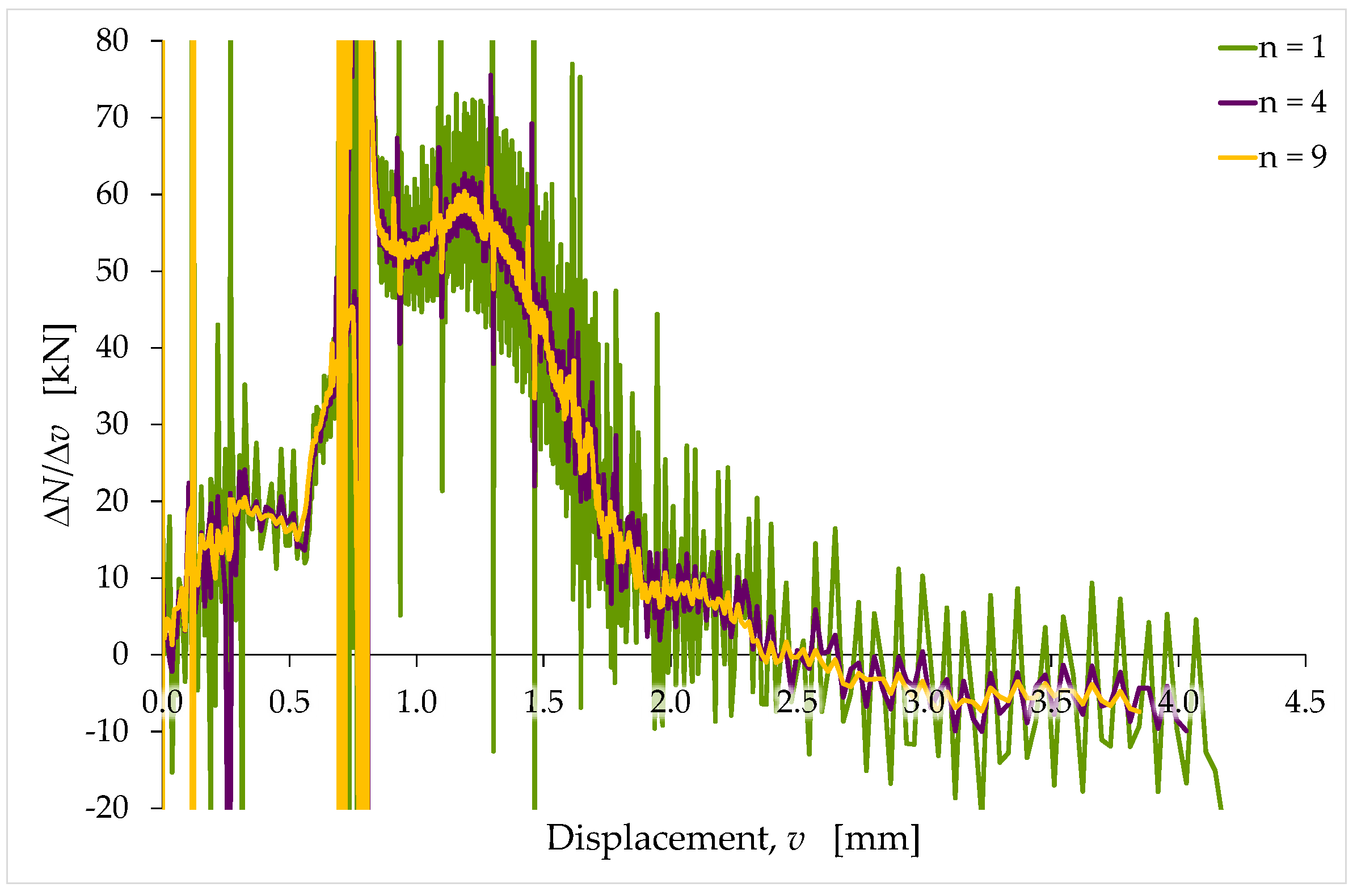
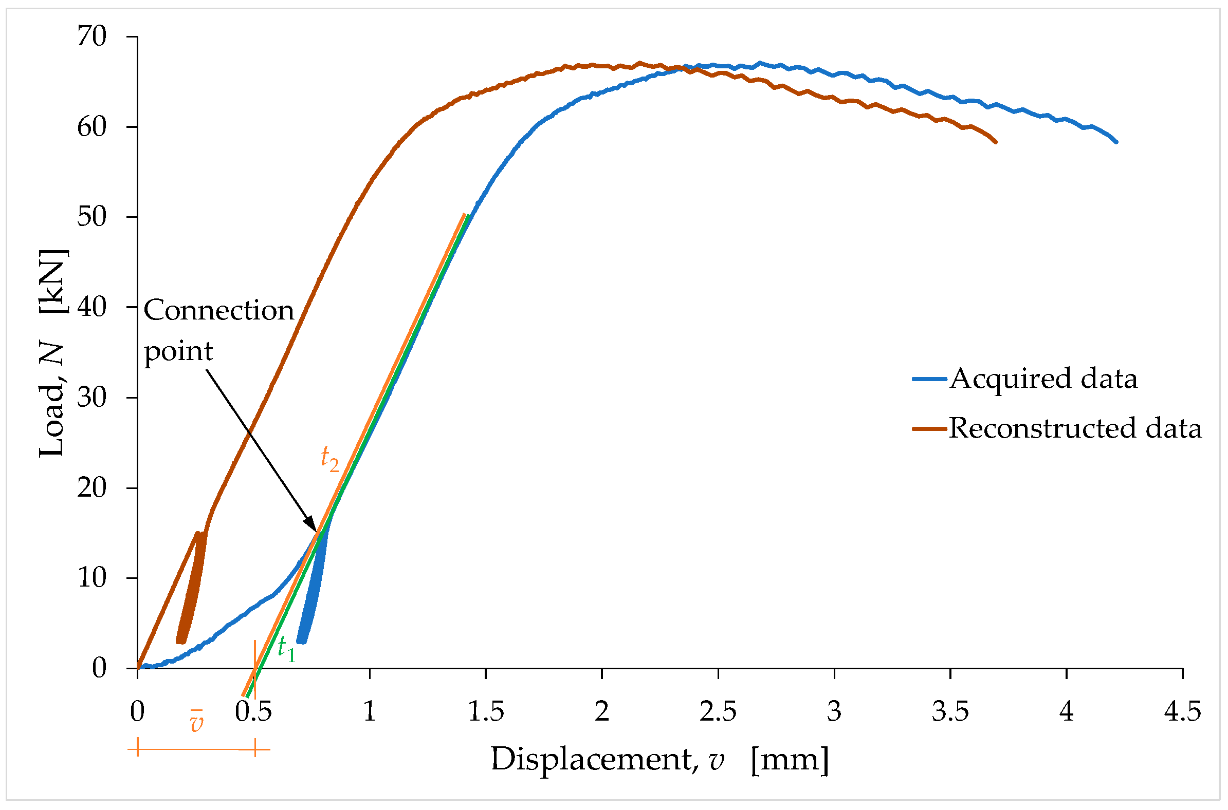
3.3. Identification of the Stiffness
- is the index of the displacement value at which to calculate . It also sets the first end of both the displacement range and the load range for the slope calculation;
- is a natural number . It sets the position of the second end—in both the displacement range and the load range—since the two ends of the displacement and load ranges for the slope calculation are not necessarily consecutive data.
4. Experimental Results and Discussion
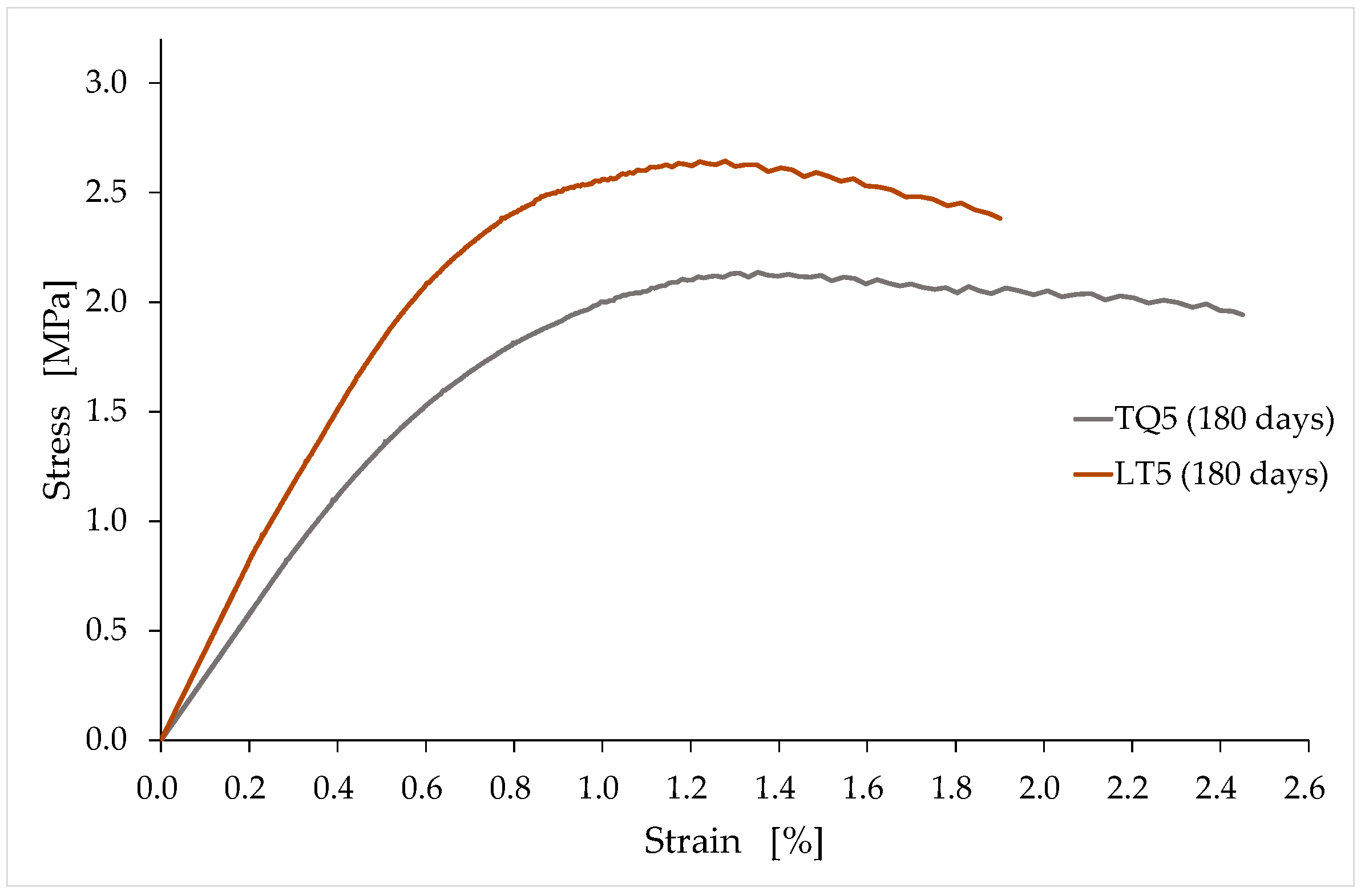
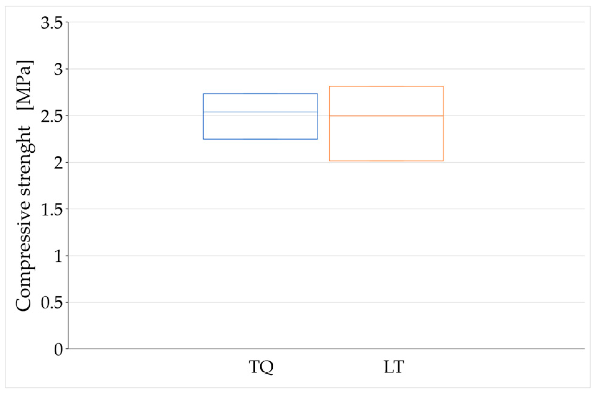
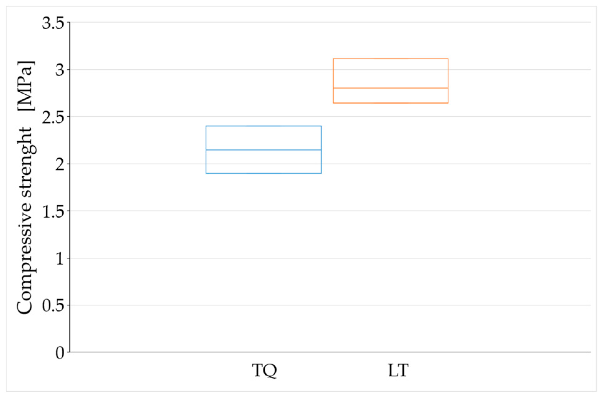
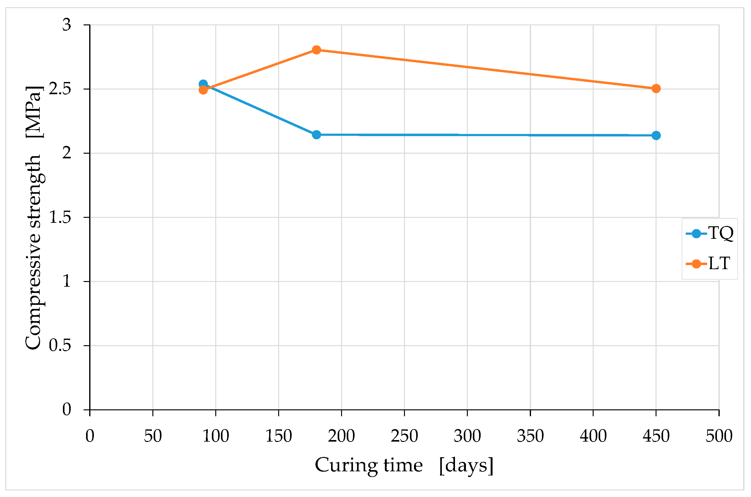
4.1. Effect of RH Shredding on Compressive Strength
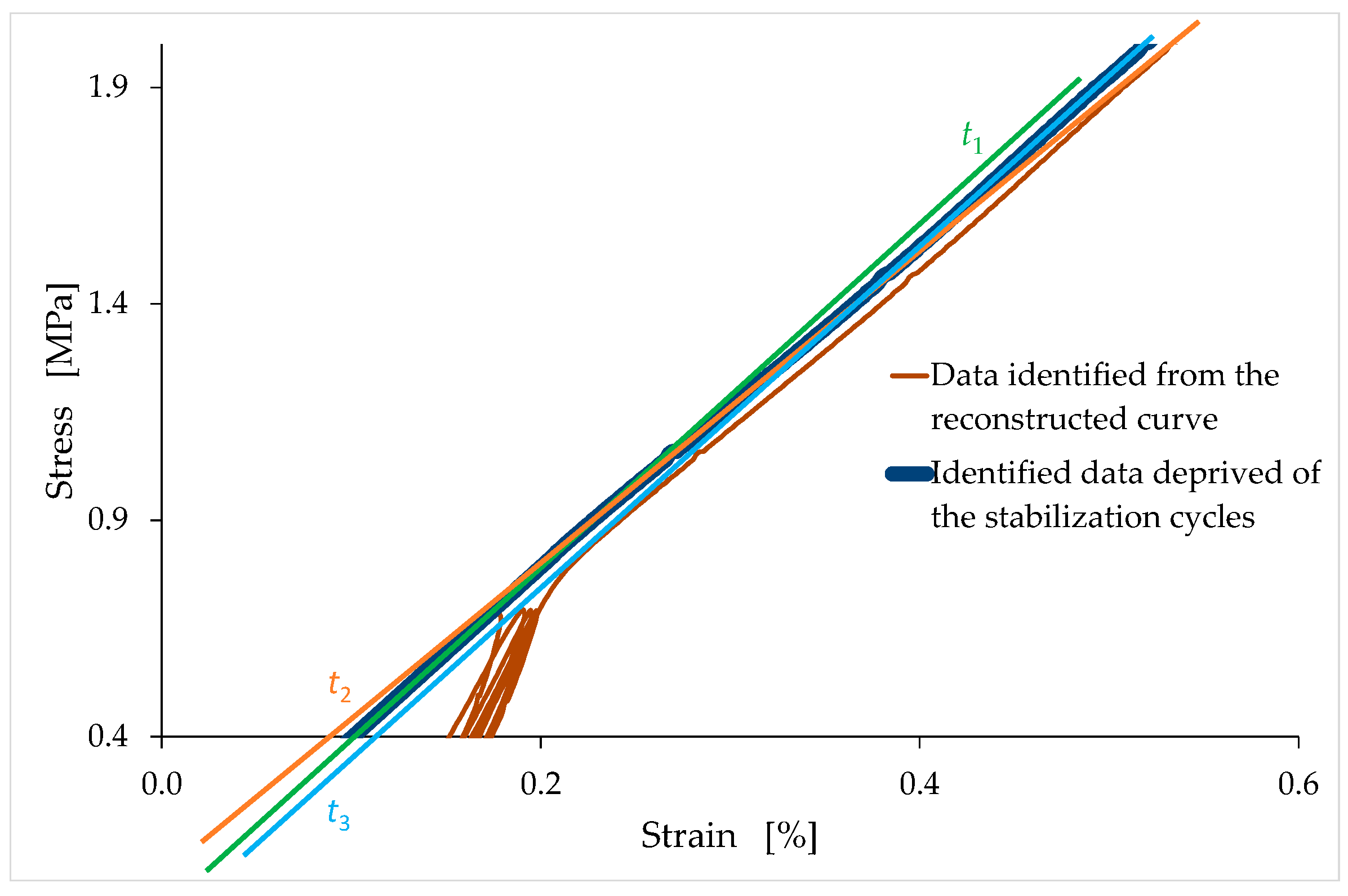
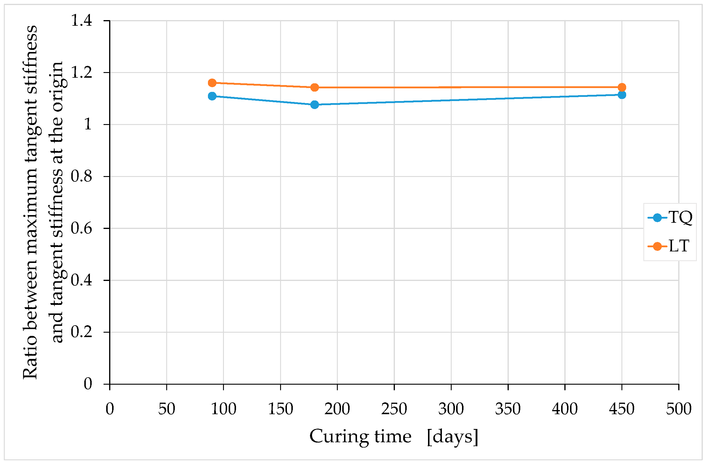
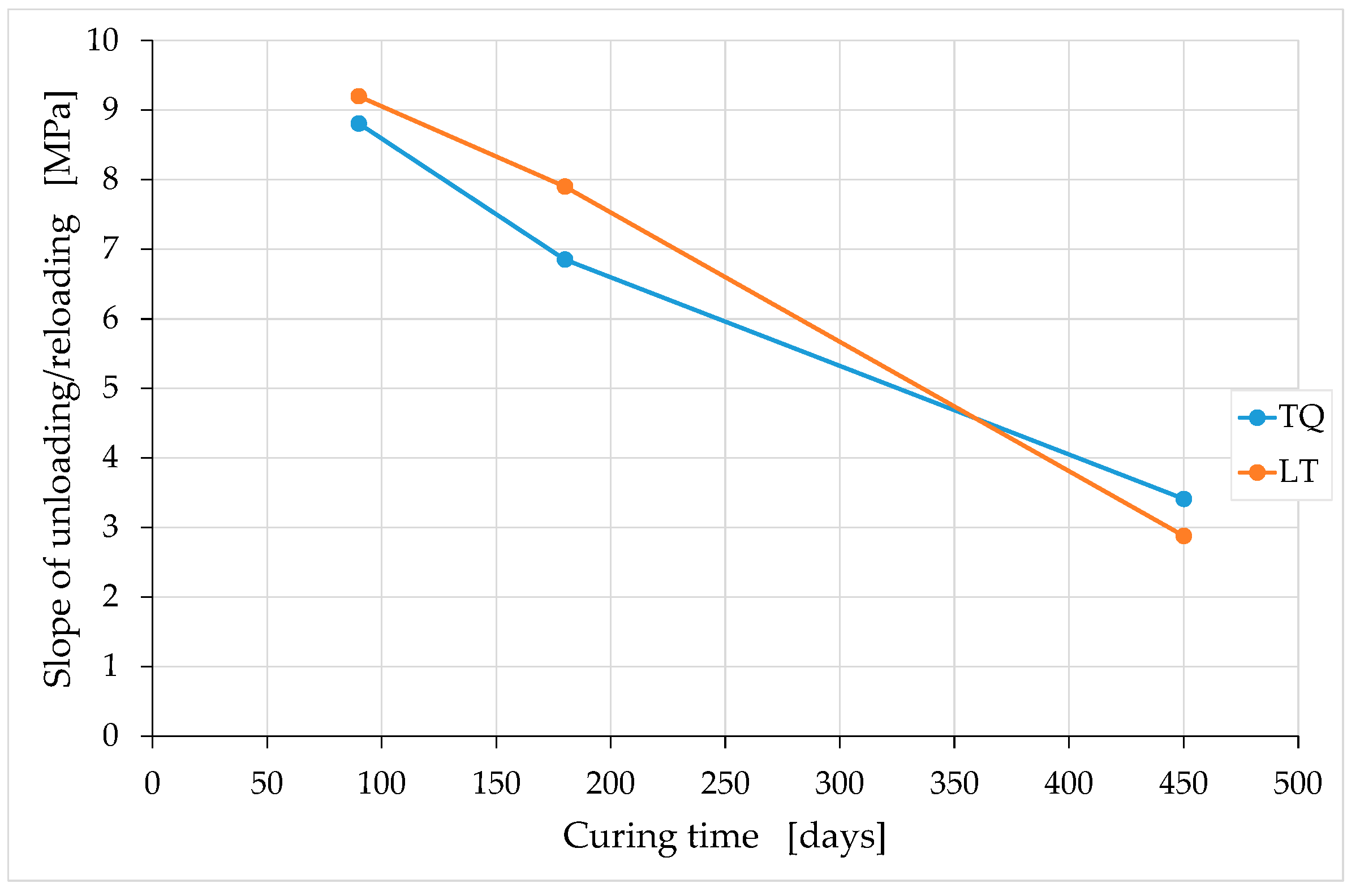
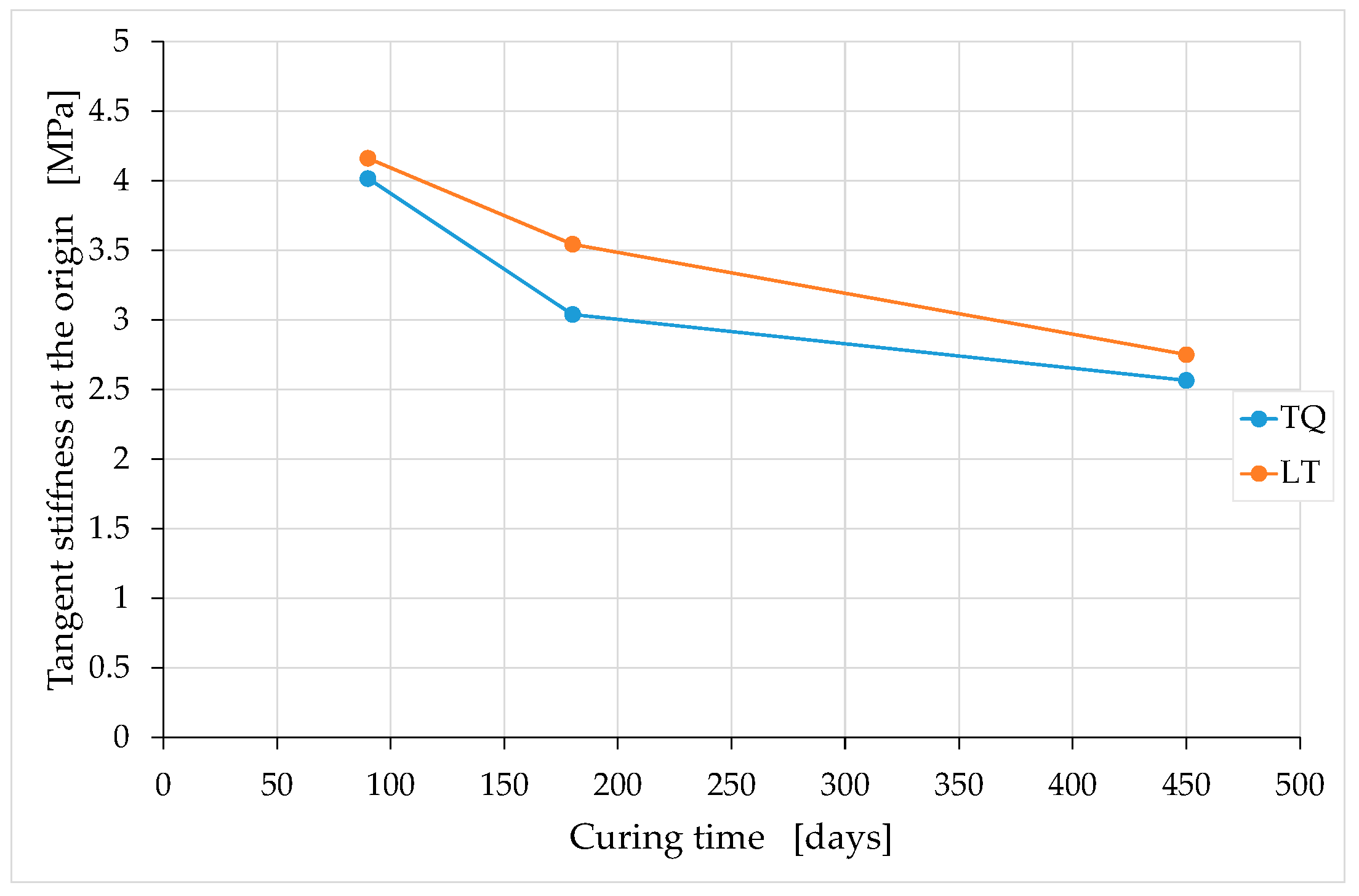
4.2. Effect of RH Shredding on Stiffness
5. Conclusions and Future Developments
Supplementary Materials
Author Contributions
Funding
Institutional Review Board Statement
Informed Consent Statement
Data Availability Statement
Acknowledgments
Conflicts of Interest
References
- Kothman, I.; Faber, N. How 3D printing technology changes the rules of the game: Insights from the construction sector. J. Manuf. Technol. Manag. 2016, 27, 932–943. [Google Scholar] [CrossRef]
- Tay, Y.W.D.; Panda, B.; Paul, S.C.; Noor Mohamed, N.A.; Tan, M.J.; Leong, K.F. 3D printing trends in building and construction industry: A review. Virtual Phys. Prototyp. 2017, 12, 261–276. [Google Scholar] [CrossRef]
- Alhumayani, H.; Gomaa, M.; Soebarto, V.; Jabi, W. Environmental assessment of large-scale 3D printing in construction: A comparative study between cob and concrete. J. Clean. Prod. 2020, 270, 122463. [Google Scholar] [CrossRef]
- Veliz Reyes, A.; Gomaa, M.; Chatzivasileiadi, A.; Jabi, W.; Wardhana, N.M. Computing craft: Early stage development of a robotically-supported 3D printing system for cob structures. In Proceedings of the 36th eCAADe Conference, Lodz University of Technology, Lodz, Poland, 19–21 September 2018; Kepczynska-Walczak, A., Bialkowski, S., Eds.; CumInCAD Papers: Lodz, Poland, 2018; Volume 1, pp. 791–800. [Google Scholar]
- Perrot, A.; Rangeard, D.; Pierre, A. Structural built-up of cement-based materials used for 3D-printing extrusion techniques. Mater. Struct. 2016, 49, 1213–1220. [Google Scholar] [CrossRef]
- Le, T.T.; Austin, S.A.; Lim, S.; Buswell, R.A.; Law, R.; Gibb, A.G.F.; Thorpe, T. Hardened properties of high-performance printing concrete. Cem. Concr. Res. 2012, 42, 558–666. [Google Scholar] [CrossRef] [Green Version]
- Ferretti, E.; Moretti, M.; Chiusoli, A.; Naldoni, L.; De Fabritiis, F.; Visonà, M. Mechanical Properties of a 3D-Printed Wall Segment Made with an Earthen Mixture. Materials 2022, 15, 438. [Google Scholar] [CrossRef]
- Perrot, A.; Rangeard, D.; Courteille, E. 3D printing of earth-based materials: Processing aspects. Constr. Build. Mater. 2018, 172, 670–676. [Google Scholar] [CrossRef]
- Gomaa, M.; Jabi, W.; Veliz Reyes, A.; Soebarto, V. 3D printing system for earth-based construction: Case study of cob. Autom. Constr. 2021, 124, 103577. [Google Scholar] [CrossRef]
- Etzion, Y.; Saller, M. Earth Construction—A Review of Needs and Methods. Arch. Sci. Rev. 1987, 30, 43–48. [Google Scholar] [CrossRef]
- Olivier, M.; Mesbah, A. Influence of different parameters on the resistance of earth, used as a building material. In Proceedings of the International Conference on Mud Architecture, Trivandrum, India, 25–27 November 1987. [Google Scholar]
- Germen, A. The endurance of earths as building material and the discreet but continuous charm of adobe. METU J. Fac. Archit. 1979, 5, 37–68. [Google Scholar]
- Keefe, L. Earth Building Methods and Materials, Repair and Conservation; Taylor & Francis: New York, NY, USA, 2005. [Google Scholar]
- Deboucha, S.; Hashim, R. A review on bricks and stabilized compressed earth blocks. Sci. Res. Essays 2011, 6, 499–506. [Google Scholar]
- Treloar, G.; Owen, C.M.; Fay, M.R. Enviromental assessment of rammed earth construction systems. Struct. Surv. 2001, 19, 99–105. [Google Scholar] [CrossRef]
- Pacheco-Torgal, F.; Jalali, S. Earth construction: Lessons from the past for future eco-efficient construction. Constr. Build. Mater. 2012, 29, 512–519. [Google Scholar] [CrossRef] [Green Version]
- Gallipoli, D.; Bruno, A.W.; Perlot, C.; Salmon, N. Raw Earth Construction: Is There a Role for Unsaturated Soil Mechanics? Taylor & Francis Group: London, UK, 2014. [Google Scholar]
- Schroeder, H. Sustainable Building with Earth; Springer International Publishing: New York, NY, USA, 2016. [Google Scholar]
- Walker, P. Editorial. Proc. Inst. Civ. Eng. Constr. Mater. 2016, 169, 239–240. [Google Scholar] [CrossRef] [Green Version]
- Olivier, M.; Mesbah, A. Le matériau terre: Essai de compactage statique pour la fabrication de briques de terre compressées. Bull. Liaison Lab. Ponts Chaussées 1986, 146, 37–43. [Google Scholar]
- Houben, H.; Guillaud, H. Earth Construction: A Comprehensive Guide; Intermediate Technology Publications: London, UK, 1994. [Google Scholar]
- Rigassi, V. CRATerre-EAG. In Compressed Earth Blocks: Manual of Production; Friedrich Vieweg & Sohn: Braunschweig, Germany, 1995. [Google Scholar]
- Walker, P. Strength, durability and shrinkage characteristics of cement stabilised soil blocks. Cem. Concr. Compos. 1995, 17, 301–310. [Google Scholar] [CrossRef]
- Maniatidis, V.; Walker, P. A Review of Rammed Earth Construction; DTi Partners in Innovation Project ‘Developing Rammed Earth for UK Housing’; University of Bath: Bath, UK, 2003; Available online: https://people.bath.ac.uk/abspw/rammedearth/review.pdf (accessed on 20 December 2021).
- Morel, J.-C.; Pkla, A.; Walker, P. Compressive strength testing of compressed earth blocks. Constr. Build. Mater. 2007, 21, 303–309. [Google Scholar] [CrossRef]
- Kouakou, C.H.; Morel, J.-C. Strength and elasto-plastic properties of non-industrial building materials manufactured with clay as a natural binder. Appl. Clay Sci. 2009, 44, 27–34. [Google Scholar] [CrossRef]
- Reddy, B.; Kumar, P.P. Cement stabilised rammed earth. Part A: Compaction characteristics and physical properties of com-pacted cement stabilised soils. Mater. Struct. 2011, 4, 681–693. [Google Scholar] [CrossRef]
- Reddy, B.; Kumar, P.P. Cement stabilised rammed earth. Part B: Compressive strength and stress–strain characteristics. Mater. Struct. 2011, 44, 695–707. [Google Scholar] [CrossRef]
- Bruno, A.W.; Gallipoli, D.; Perlot, C.; Mendes, J. Effect of very high compaction pressures on the physical and mechanical properties of earthen materials. In Proceedings of the 3rd European Conference on Unsaturated Soils, Paris, France, 12–14 September 2016; Volume 9, p. 14004. [Google Scholar]
- McGregor, F.; Heath, A.; Fodde, E.; Shea, A. Conditions affecting the moisture buffering measurement performed on compressed earth blocks. Build. Environ. 2014, 75, 11–18. [Google Scholar] [CrossRef] [Green Version]
- Fabbri, A.; Morel, J.-C.; Gallipoli, D. Assessing the performance of earth building materials: A review of recent developments. RILEM Tech. Lett. 2018, 3, 46–58. [Google Scholar] [CrossRef]
- Verma, P.L.; Mehra, S.R. Use of soil-cement in house construction in the Punjab. Indian Concr. J. 1950, 24, 91–96. [Google Scholar]
- Walker, P. HB 195: The Australian Earth Building Handbook; Standards Australia: Sydney, Australia, 2002. [Google Scholar]
- Walker, P.; Keable, R.; Martin, J.; Maniatidis, V. Rammed Earth: Design and Construction Guidelines; IHS BRE: Watford, UK, 2005. [Google Scholar]
- Fitzmaurice, R. Manual on Stabilized Soil Construction for Housing; Technical Assistance Programme; United Nations: New York, NY, USA, 1958. [Google Scholar]
- Spence, R.J.S. Predicting the performance of soil-cement as a building material in tropical countries. Build. Sci. 1975, 10, 155–159. [Google Scholar] [CrossRef]
- Alley, P.J. Rammed Earth Construction. N. Z. Eng. 1948, 3, 582. [Google Scholar]
- McHenry, P.G. Adobe and Rammed Earth Buildings: Design and Construction; The University of Arizona Press: Tucson, AZ, USA, 1984. [Google Scholar]
- Koutous, A.; Hilali, E.M. A Proposed Experimental Method for the Preparation of Rammed Earth Material. Int. J. Eng. Tech. Res. (IJERT) 2019, 8, 345–354. [Google Scholar] [CrossRef]
- Smith, E.W.; Austin, G.S. Adobe, Pressed-Earth, and Rammed-Earth Industries in New Mexico; Bulletin 127; New Mexico Bureau of Mines & Mineral Resources: Socorro, NM, USA, 1989. [Google Scholar]
- Norton, J. Building with Earth: A Handbook, 2nd ed.; Intermediate Technology Publications: London, UK, 1997. [Google Scholar]
- Gooding, D. Soil Testing for Soil-Cement Block Preparation; DTU Working Paper: WP38; University of Warwick: Coventry, UK, 1993. [Google Scholar]
- Montgomery, D. Physical Characteristics of Soils that Encourage SSB Breakdown during Moisture Attack; Stabilised Soil Research Progress Report SSRPR03; University of Warwick: Coventry, UK, 1998. [Google Scholar]
- Volunteers in Technical Assistance (VITA). Making Buildings Blocks with the CINVA-Ram Block Press, Volunteers in Technical Assistance, 3rd ed.; Intermediate Technology Publications: London, UK, 1975. [Google Scholar]
- Reddy, B.; Jagadish, K.S. Influence of soil composition on the strength and durability of soil-cement blocks. Indian Concr. J. 1995, 69, 517–524. [Google Scholar]
- Walker, P.; Stace, T. Properties of some cement stabilised compressed earth blocks and mortars. Mater. Struct. 1997, 30, 545–551. [Google Scholar] [CrossRef]
- Reddy, B.; Lal, R.; Rao, K.N. Optimum Soil Grading for the Soil-Cement Blocks. J. Mater. Civ. Eng. 2007, 19, 139–148. [Google Scholar] [CrossRef]
- Reddy, B.; Latha, M.S. Influence of soil grading on the characteristics of cement stabilised soil compacts. Mater. Struct. 2014, 47, 1633–1645. [Google Scholar] [CrossRef]
- Burroughs, S. Soil Property Criteria for Rammed Earth Stabilization. J. Mater. Civ. Eng. 2008, 20, 264–273. [Google Scholar] [CrossRef]
- Burroughs, S. Recommendations for the Selection, Stabilization, and Compaction of Soil for Rammed Earth Wall Construction. J. Green Build. 2010, 5, 101–114. [Google Scholar] [CrossRef]
- Reddy, B.; Kumar, P.P. Role of clay content and moisture on characteristics of cement stabilised rammed earth. In Proceedings of the 11th International Conference on Non-Conventional Materials and Technologies (NOCMAT), Bath University, Bath, UK, 6–9 September 2009. [Google Scholar]
- Nagaraj, H.B.; Rajesh, A.; Sravan, M.V. Influence of soil gradation, proportion and combination of admixtures on the prop-erties and durability of CSEBs. Constr. Build. Mater. 2016, 110, 135–144. [Google Scholar] [CrossRef]
- Bryan, A.J. Criteria for the suitability of soil for cement stabilization. Build. Environ. 1988, 23, 309–319. [Google Scholar] [CrossRef]
- Reddy, B.; Jagadish, K.S. Properties of soil–cement block masonry. Mason. Int. 1989, 3, 80–84. [Google Scholar]
- Ciancio, D.; Boulter, M. Stabilised rammed earth: A case study in Western Australia. Proc. Inst. Civ. Eng. Eng. Sustain. 2012, 165, 141–154. [Google Scholar] [CrossRef]
- Heathcote, K.A. Durability of earthwall buildings. Constr. Build. Mater. 1995, 9, 185–189. [Google Scholar] [CrossRef]
- Morel, J.-C.; Bui, Q.B.; Hamard, E. Weathering and durability of earthen material and structures. In Modern Earth Buildings: Materials, Engineering, Constructions and Applications; Hall, M.R., Lindsay, R., Krayenhoff, M., Eds.; Woodhead Publishing: Cambridge, UK, 2012; pp. 282–303. [Google Scholar]
- Guettala, A.; Abibsi, A.; Houari, H. Durability study of stabilized earth concrete under both laboratory and climatic conditions exposure. Constr. Build. Mater. 2006, 20, 119–127. [Google Scholar] [CrossRef]
- Bui, Q.B.; Morel, J.-C.; Venkatarama Reddy, B.V.; Ghayad, W. Durability of rammed earth walls exposed for 20 years to nat-ural weathering. Build. Environ. 2009, 44, 912–919. [Google Scholar] [CrossRef]
- Beckett, C.; Ciancio, D. Durability of cement-stabilised rammed earth: A case study in Western Australia. Aust. J. Civ. Eng. 2016, 14, 54–62. [Google Scholar] [CrossRef] [Green Version]
- Bruno, A.W.; Gallipoli, D.; Perlot, C.; Mendes, J. Effect of stabilisation on mechanical properties, moisture buffering and water durability of hypercompacted earth. Constr. Build. Mater. 2017, 149, 733–740. [Google Scholar] [CrossRef]
- Allinson, D.; Hall, M. Humidity buffering using stabilised rammed earth materials. Proc. Inst. Civ. Eng. Constr. Mater. 2012, 165, 335–344. [Google Scholar] [CrossRef] [Green Version]
- McGregor, F.; Heath, A.; Shea, A.; Lawrence, M. The moisture buffering capacity of unfired clay masonry. Build. Environ. 2014, 82, 599–607. [Google Scholar] [CrossRef] [Green Version]
- Oudhof, N.; Labat, M.; Magniont, C.; Nicot, P. Measurement of the hygrothermal properties of straw-clay mixtures. In Proceedings of the First International Conference on Bio-based Building Materials, Clermont Ferrand, France, 22–24 June 2015; Amziane, S., Sonebi, M., Eds.; RILEM Publications—Curran Associates, Inc.: New York, NY, USA, 2017; pp. 474–479. [Google Scholar]
- Arrigoni, A.; Grillet, A.C.; Pelosato, R.; Dotelli, G.; Beckett, C.; Woloszyn, M.; Ciancio, D. Reduction of rammed earth’s hy-groscopic performance under stabilisation: An experimental investigation. Build. Environ. 2017, 115, 358–367. [Google Scholar] [CrossRef]
- Muguda Viswanath, S. Biopolymer Stabilised Earthen Construction Materials. Ph.D. Thesis, Durham University, Durham, UK, 2019. [Google Scholar]
- Webb, D. Stabilised soil and the built environment. Renew. Energy 1994, 5, 1066–1080. [Google Scholar] [CrossRef]
- Walker, P. Editorial. Proc. Inst. Civ. Eng. Constr. Mater. 2017, 170, 1–2. [Google Scholar] [CrossRef] [Green Version]
- Readle, D.; Coghlan, S.; Smith, J.C.; Corbin, A.; Augarde, C.E. Fibre reinforcement in earthen construction materials. Proc. Inst. Civ. Eng. Constr. Mater. 2016, 169, 252–260. [Google Scholar] [CrossRef] [Green Version]
- Plank, J. Applications of biopolymers and other biotechnological products in building materials. Appl. Microbiol. Biotechnol. 2004, 66, 1–9. [Google Scholar] [CrossRef]
- Yang, F.; Zhang, B.; Ma, Q. Study of sticky rice−Lime mortar technology for the restoration of historical masonry construction. Acc. Chem. Res. 2010, 43, 936–944. [Google Scholar] [CrossRef] [PubMed]
- Maskell, D.; Heath, A.; Walker, P. Comparing the Environmental Impact of Stabilisers for Unfired Earth Construction. Key Eng. Mater. 2014, 600, 132–143. [Google Scholar] [CrossRef] [Green Version]
- Reddy, B.; Kumar, P.P. Embodied energy in cement stabilised rammed earth walls. Energy Build. 2010, 42, 380–385. [Google Scholar] [CrossRef]
- Gallipoli, D.; Bruno, A.W.; Perlot, C.; Mendes, J. A geotechnical perspective of raw earth building. Acta Geotech. 2017, 12, 463–478. [Google Scholar] [CrossRef] [Green Version]
- Lax, C. Life Cycle Assessment of Rammed Earth. Master’s Thesis, University of Bath, Bath, UK, 2010. [Google Scholar]
- Fujita, Y.; Ferris, F.G.; Lawson, R.D.; Colwell, F.S.; Smith, R.W. Subscribed content calcium carbonate precipitation by ureolytic subsurface bacteria. Geomicrobiol. J. 2000, 17, 305–318. [Google Scholar] [CrossRef]
- Renforth, P.; Manning, D.A.C.; Lopez-Capel, E. Carbonate precipitation in artificial soils as a sink for atmospheric carbon dioxide. Appl. Geochem. 2009, 24, 1757–1764. [Google Scholar] [CrossRef]
- Ivanov, V.; Stabnikov, V. Construction Biotechnology: Biogeochemistry, Microbiology and Biotechnology of Construction Materials and Processes; Springer: Singapore, 2016. [Google Scholar]
- Cabalar, A.F.; Canakci, H. Direct shear tests on sand treated with xanthan gum. Proc. Inst. Civ. Eng. Ground Improv. 2011, 164, 57–64. [Google Scholar] [CrossRef]
- Chen, R.; Zhang, L.; Budhu, M. Biopolymer Stabilization of Mine Tailings. J. Geotech. Geoenvironmental Eng. 2013, 139, 1802–1807. [Google Scholar] [CrossRef]
- Chang, I.; Im, J.; Prasidhi, A.K.; Cho, G.-C. Effects of Xanthan gum biopolymer on soil strengthening. Constr. Build. Mater. 2015, 74, 65–72. [Google Scholar] [CrossRef]
- Chang, I.; Prasidhi, A.K.; Im, J.; Cho, G.-C. Soil strengthening using thermo-gelation biopolymers. Constr. Build. Mater. 2015, 77, 430–438. [Google Scholar] [CrossRef]
- Aguilar, R.; Nakamatsu, J.; Ramírez, E.; Elgegren, M.; Ayarza, J.; Kim, S.; Pando, M.A.; Ortega-San-Martin, L. The potential use of chitosan as a biopolymer additive for enhanced mechanical properties and water resistance of earthen construction. Constr. Build. Mater. 2016, 114, 625–637. [Google Scholar] [CrossRef]
- Ayeldeen, M.K.; Negm, A.M.; El Sawwaf, M.A. Evaluating the physical characteristics of biopolymer/soil mixtures. Arab. J. Geosci. 2016, 9, 329–339. [Google Scholar] [CrossRef]
- Pacheco-Torgal, F.; Ivanov, V.; Karak, N.; Jonkers, H. Biopolymers and Biotech Admixtures for Eco-Efficient Construction Materials; Woodhead Publishing: Sawston, UK, 2016. [Google Scholar]
- Latifi, N.; Horpibulsuk, S.; Meehan, C.L.; Abd Majid, M.Z.; Tahir, M.M.; Mohamad, E.T. Improvement of Problematic Soils with Biopolymer—An Environmentally Friendly Soil Stabilizer. J. Mater. Civ. Eng. 2017, 29, 04016204. [Google Scholar] [CrossRef]
- Nakamatsu, J.; Kim, S.; Ayarza, J.; Ramírez, E.; Elgegren, M.; Aguilar, R. Eco-friendly modification of earthen construction with carrageenan: Water durability and mechanical assessment. Constr. Build. Mater. 2017, 139, 193–202. [Google Scholar] [CrossRef]
- Qureshi, M.U.; Chang, I.; Al-Sadarani, K. Strength and durability characteristics of biopolymer-treated desert sand. Géoméch. Eng. 2017, 12, 785–801. [Google Scholar] [CrossRef]
- Chen, C.; Wu, L.; Perdjon, M.; Huang, X.; Peng, Y. The drying effect on xanthan gum biopolymer treated sandy soil shear strength. Constr. Build. Mater. 2019, 197, 271–279. [Google Scholar] [CrossRef] [Green Version]
- Chang, I.; Im, J.; Cho, G.-C. Introduction of Microbial Biopolymers in Soil Treatment for Future Environmentally-Friendly and Sustainable Geotechnical Engineering. Sustainability 2016, 8, 251. [Google Scholar] [CrossRef] [Green Version]
- Stabnikov, V.; Ivanov, V.; Chu, J. Construction Biotechnology: A new area of biotechnological research and applications. World J. Microbiol. Biotechnol. 2015, 31, 1303–1314. [Google Scholar] [CrossRef] [PubMed]
- Komnitsas, K.; Zaharaki, D. Geopolymerisation: A review and prospects for the minerals industry. Miner. Eng. 2007, 20, 1261–1277. [Google Scholar] [CrossRef]
- De Silva, P.; Sagoe-Crenstil, K.; Sirivivatnanon, V. Kinetics of geopolymerization: Role of Al2O3 and SiO2. Cem. Concr. Res. 2007, 37, 512–518. [Google Scholar] [CrossRef]
- Fletcher, R.A.; MacKenzie, K.J.; Nicholson, C.L.; Shimada, S. The composition range of aluminosilicate geopolymers. J. Eur. Ceram. Soc. 2005, 25, 1471–1477. [Google Scholar] [CrossRef]
- Songpiriyakij, S.; Kubprasit, T.; Jaturapitakkul, C.; Chindaprasirt, P. Compressive strength and degree of reaction of bio-mass-and fly ash-based geopolymer. Constr. Build. Mater. 2010, 24, 236–240. [Google Scholar] [CrossRef]
- Cheng, T.-W.; Chiu, J. Fire-resistant geopolymer produced by granulated blast furnace slag. Miner. Eng. 2003, 16, 205–210. [Google Scholar] [CrossRef]
- Colombo, D. WASP Arriva a 12 Metri. 2015. Available online: https://www.01factory.it/wasp-arriva-a-12-metri (accessed on 20 December 2021).
- Colombo, D. La BigDelta di WASP nel Parco Della Stampa 3D. 2016. Available online: https://www.01factory.it/la-bigdelta-di-wasp-nel-parco-della-stampa-3d (accessed on 20 December 2021).
- Colombo, D. Tecla, la Casa Stampata in 3D in Terra Cruda. 2021. Available online: https://www.01building.it/progetti/tecla-casa-stampata-3d-terra-cruda (accessed on 20 December 2021).
- Singh, B. Rice husk ash. In Waste and Supplementary Cementitious Materials in Concrete; Elsevier: Amsterdam, The Netherlands, 2018; pp. 417–460. [Google Scholar]
- Omatola, K.; Onojah, A. Rice Husk as a Potential Source of High Technology Raw Materials: A Review. J. Phys. Sci. Innov. 2012, 4, 1–6. [Google Scholar]
- Mathur, A.; Singh, U.; Vijay, Y.; Hemlata, M.S.; Sharma, M. Analysing performance for generating power with renewable energy source using rice husk as an alternate fuel. Control Theory Inform. 2013, 3, 64–71. [Google Scholar]
- Mohd Basri, M.S.; Mustapha, F.; Mazlan, N.; Ishak, M.R. Rice Husk Ash-based Geopolymer Binder: Compressive Strength, Optimize Composition, FTIR Spectroscopy, Microstructural and Potential as Fire Retardant Material. Polymers 2021, 13, 4373. [Google Scholar] [CrossRef] [PubMed]
- Moretti, M.; Chiusoli, A.; Naldoni, L.; De Fabritiis, F.; Visonà, M. Earthen 3d printed constructions towards a new high-efficient way of building. In Past and Present of the Earthen Architectures in China and Italy; Luvidi, L., Fratini, F., Rescic, S., Zhang, J., Eds.; Cnr Edizioni: Roma, Italy, 2021; pp. 147–155. [Google Scholar]
- Cengiz, O.; Chen, Y.; Datta, I.; Du, Y.; Foroughi, A.; Kriki, P.; Liao, Y.F.; Loonawat, B.V.; Randeria, S.C.; Salahinejhad, P.; et al. Architecture of Continuity: From Materiality to Environment—Open Thesis Fabrication 2018–2019; Iaac: Barcelona, Spain, 2019. [Google Scholar]
- Walker, P. Characteristics of Pressed Earth Blocks in Earth Blocks. In Proceedings of the 11th International Brick/Block Masonry Conference, Tonji University, Shanghai, China, 14–16 October 1997; pp. 14–16. [Google Scholar]
- Aubert, J.E.; Maillard, P.; Morel, J.-C.; Al Rafii, M. Towards a simple compressive strength test for earth bricks? Mater. Struct. 2016, 49, 1641–1654. [Google Scholar] [CrossRef]
- Ferretti, E.; Di Leo, A.; Viola, E. A novel approach for the identification of material elastic constants. In CISM Courses and Lecture—sProblems in Structural Identification and Diagnostics: General Aspects and Applications, Proceedings of the Workshop on Problems in Structural Identification and Diagnostics, Bologna, Italy, 15–16 July 2002; Davini, C., Viola, E., Eds.; Springer: Vienna, Austria, 2003; Volume 471, pp. 117–131. [Google Scholar]
- Ferretti, E. Experimental procedure for verifying strain-softening in concrete. Int. J. Fract. 2004, 126, L27–L34. [Google Scholar] [CrossRef]
- Ferretti, E. On nonlocality and locality: Differential and discrete formulations. In Proceedings of the 11th International Conference on Fracture 2005, Turin, Italy, 20–25 March 2005; International Congress on Fracture (ICF)—Curran Associates, Inc.: New York, NY, USA, 2010; Volume 3, pp. 1728–1733. [Google Scholar]
- Ferretti, E.; Di Leo, A. Cracking and creep role in displacements at constant load: Concrete solids in compression. CMC-Comput. Mater. Continua. 2008, 7, 59–79. [Google Scholar]
- Ferretti, E. Shape-effect in the effective laws of plain and rubberized concrete. CMC-Comput. Mater. Continua. 2012, 30, 237–284. [Google Scholar]
- Ferretti, E. A discussion of strain-softening in concrete. Int. J. Fract. 2004, 126, L3–L10. [Google Scholar] [CrossRef]
- Ferretti, E. On Strain-softening in Dynamics. Int. J. Fract. 2004, 126, L75–L82. [Google Scholar] [CrossRef]
- Ferretti, E. The Cell Method: An enriched description of physics starting from the algebraic formulation. CMC-Comput. Mater. Continua 2013, 36, 49–71. [Google Scholar]
- Ferretti, E.; Di Leo, A.; Viola, E. Computational aspects and numerical simulations in the elastic constants identification. In CISM Courses and Lectures Problems in Structural Identification and Diagnostics: General Aspects and Applications, Proceedings of the Workshop on Problems in Structural Identification and Diagnostics, Bologna, Italy, 15–16 July 2002; Dav-ini, C., Viola, E., Eds.; Springer: Vienna, Austria, 2003; Volume 471, pp. 133–147. [Google Scholar]
- Saadeldin, R.; Siddiqua, S. Geotechnical characterization of a clay–cement mix. Bull. Eng. Geol. Environ. 2013, 72, 601–608. [Google Scholar] [CrossRef]
- Porbaha, A.; Shibuya, S.; Kishida, T. State of the art in deep mixing technology. Ground. Improv. 2000, 4, 91–110. [Google Scholar] [CrossRef]
- Horpibulsk, S.; Rachan, R.; Suddeepong, A.; Chinkulkijniwat, A. Strength Development in Cement Admixed Bangkok Clay: Laboratory and Field Investigations. Soils Found. 2011, 51, 239–251. [Google Scholar] [CrossRef] [Green Version]
- Bergado, D.T.; Anderson, L.R.; Miura, N.; Balasubramaniam, A.S. Soft Ground Improvement in Lowland and Other Environments; ASCE Press: New York, NY, USA, 1996. [Google Scholar]


| Component | TQ Mix | LT Mix |
|---|---|---|
| Soil | 70.42% | 70.42% |
| Lime-based binder | 4.70% | 4.70% |
| Hydraulic lime | 4.69% | 4.69% |
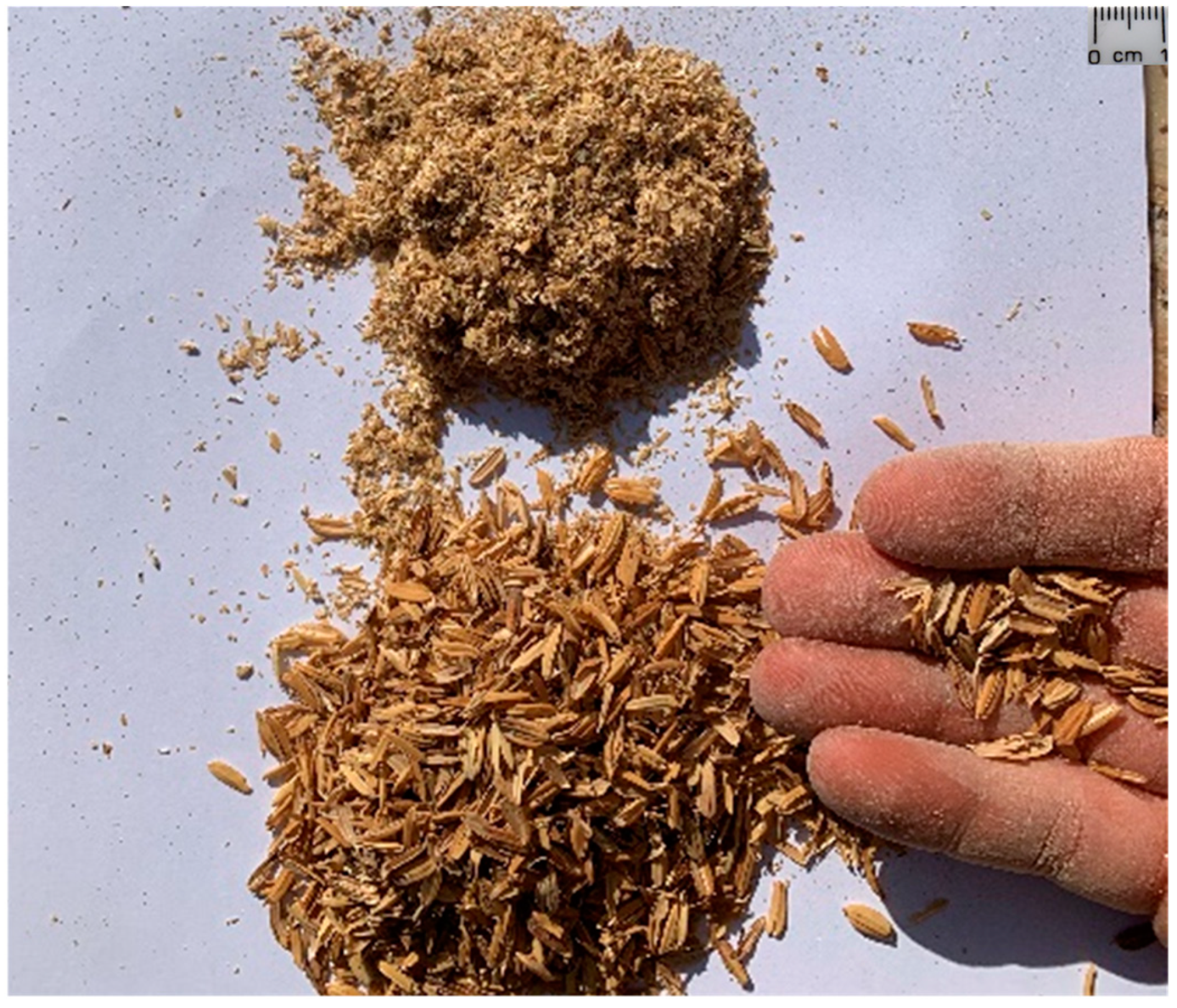
| Unaltered rice husk | 1.41% | / |
| Shredded rice husk | / | 1.41% |
| Silica sand | 18.78% | 18.78% |
| Opening Diameter (mm) | Cumulative Retained (%) |
|---|---|
| 8 | 0 |
| 4 | 0.1 |
| 2 | 0.5 |
| 1 | 1.0 |
| 0.4 | 2.0 |
| 0.075 | 7.1 |
| 0.001 | 100 |
| Specimen Label | Type of Mixture | Curing Days |
|---|---|---|
| TQ1 | TQ mix | 90 |
| TQ2 | TQ mix | 90 |
| TQ3 | TQ mix | 90 |
| TQ4 | TQ mix | 180 |
| TQ5 | TQ mix | 180 |
| TQ6 | TQ mix | 180 |
| TQ10 | TQ mix | 450 |
| TQ11 | TQ mix | 450 |
| TQ12 | TQ mix | 450 |
| LT1 | LT mix | 90 |
| LT2 | LT mix | 90 |
| LT3 | LT mix | 90 |
| LT4 | LT mix | 180 |
| LT5 | LT mix | 180 |
| LT6 | LT mix | 180 |
| LT7 | LT mix | 450 |
| LT8 | LT mix | 450 |
| LT9 | LT mix | 450 |
| Mixture | [kg/m3] | [kg/m3] | [kg/m3] | [%] |
|---|---|---|---|---|
| TQ mix | 1418.116 | 1495.728 | 1446.360 | 3.4 |
| LT mix | 1422.778 | 1494.151 | 1446.687 | 3.3 |
Publisher’s Note: MDPI stays neutral with regard to jurisdictional claims in published maps and institutional affiliations. |
© 2022 by the authors. Licensee MDPI, Basel, Switzerland. This article is an open access article distributed under the terms and conditions of the Creative Commons Attribution (CC BY) license (https://creativecommons.org/licenses/by/4.0/).
Share and Cite
Ferretti, E.; Moretti, M.; Chiusoli, A.; Naldoni, L.; de Fabritiis, F.; Visonà, M. Rice-Husk Shredding as a Means of Increasing the Long-Term Mechanical Properties of Earthen Mixtures for 3D Printing. Materials 2022, 15, 743. https://doi.org/10.3390/ma15030743
Ferretti E, Moretti M, Chiusoli A, Naldoni L, de Fabritiis F, Visonà M. Rice-Husk Shredding as a Means of Increasing the Long-Term Mechanical Properties of Earthen Mixtures for 3D Printing. Materials. 2022; 15(3):743. https://doi.org/10.3390/ma15030743
Chicago/Turabian StyleFerretti, Elena, Massimo Moretti, Alberto Chiusoli, Lapo Naldoni, Francesco de Fabritiis, and Massimo Visonà. 2022. "Rice-Husk Shredding as a Means of Increasing the Long-Term Mechanical Properties of Earthen Mixtures for 3D Printing" Materials 15, no. 3: 743. https://doi.org/10.3390/ma15030743
APA StyleFerretti, E., Moretti, M., Chiusoli, A., Naldoni, L., de Fabritiis, F., & Visonà, M. (2022). Rice-Husk Shredding as a Means of Increasing the Long-Term Mechanical Properties of Earthen Mixtures for 3D Printing. Materials, 15(3), 743. https://doi.org/10.3390/ma15030743