
Specifications for Modelling of the Phenomenon of Compression of Closed-Cell Aluminium Foams with Neural Networks


Abstract
1. Introduction
1.1. Problem Origins
1.2. Problem Statement and Proposed Solution’s Generals
1.3. Research Significance
- Is it possible to describe the phenomenon of compression of aluminium foams with a model generated from neural networks based on the assumed general relation?
- What assumptions/general choices about the networks’ structure and learning parameters should be determined?
- How should the obtained results be evaluated? What criteria and what measures should be assumed?
- What structure and learning parameters should be assumed to most adequately describe the phenomenon?
- Is the model valid only for the training data (particular model), or is it capable of prognosing for new data (general model)?
2. Material and Experiment
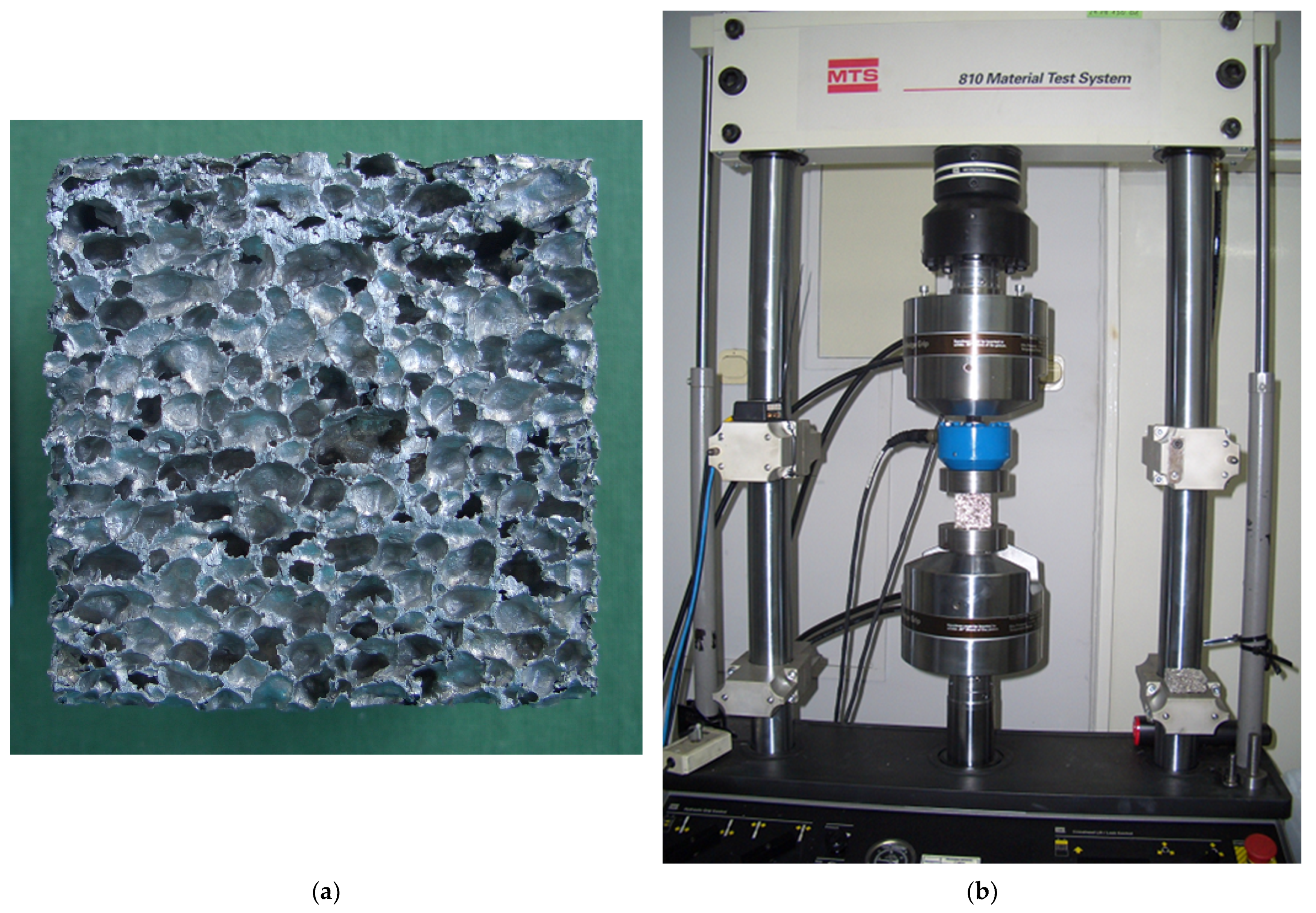
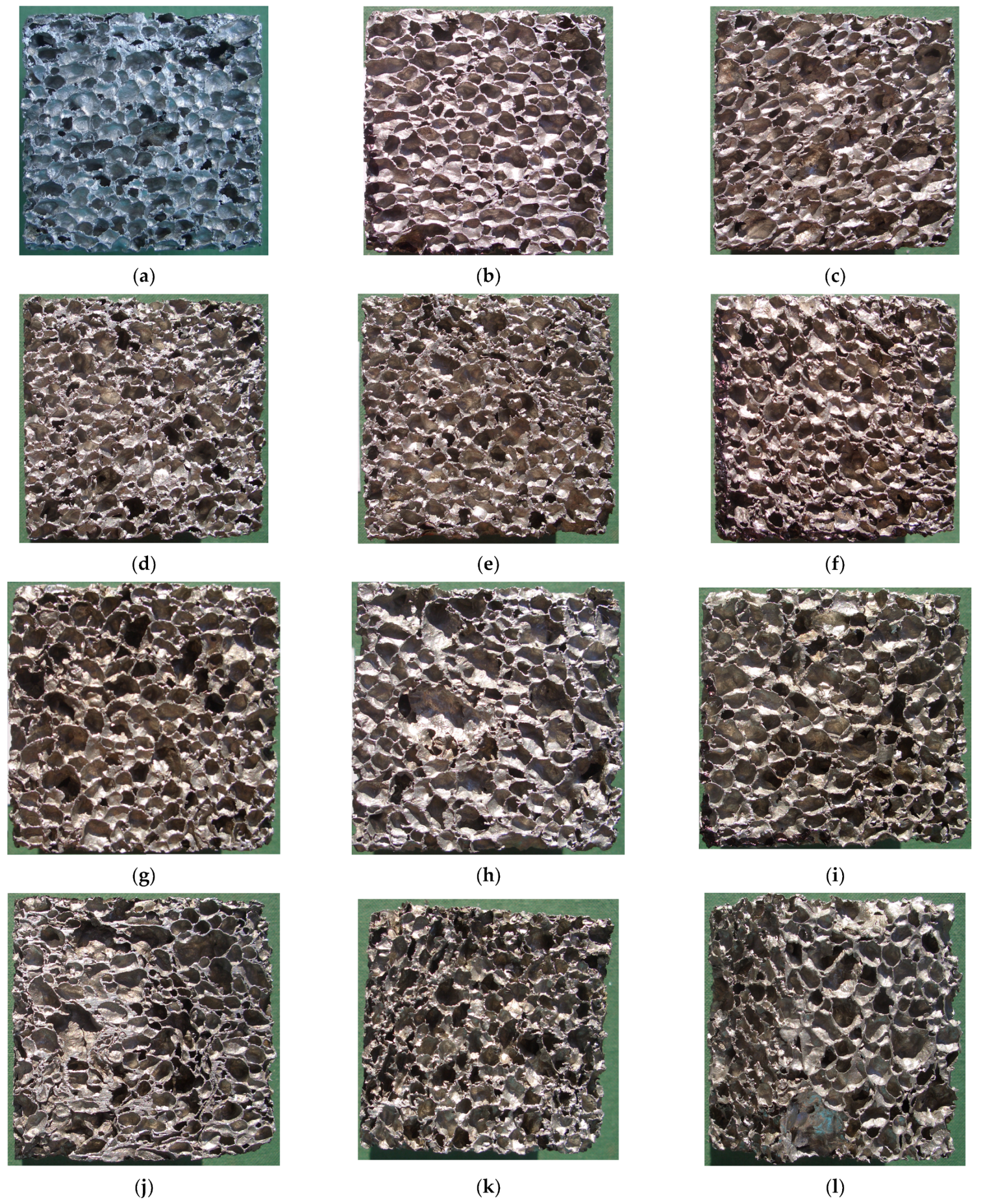
2.1. Material
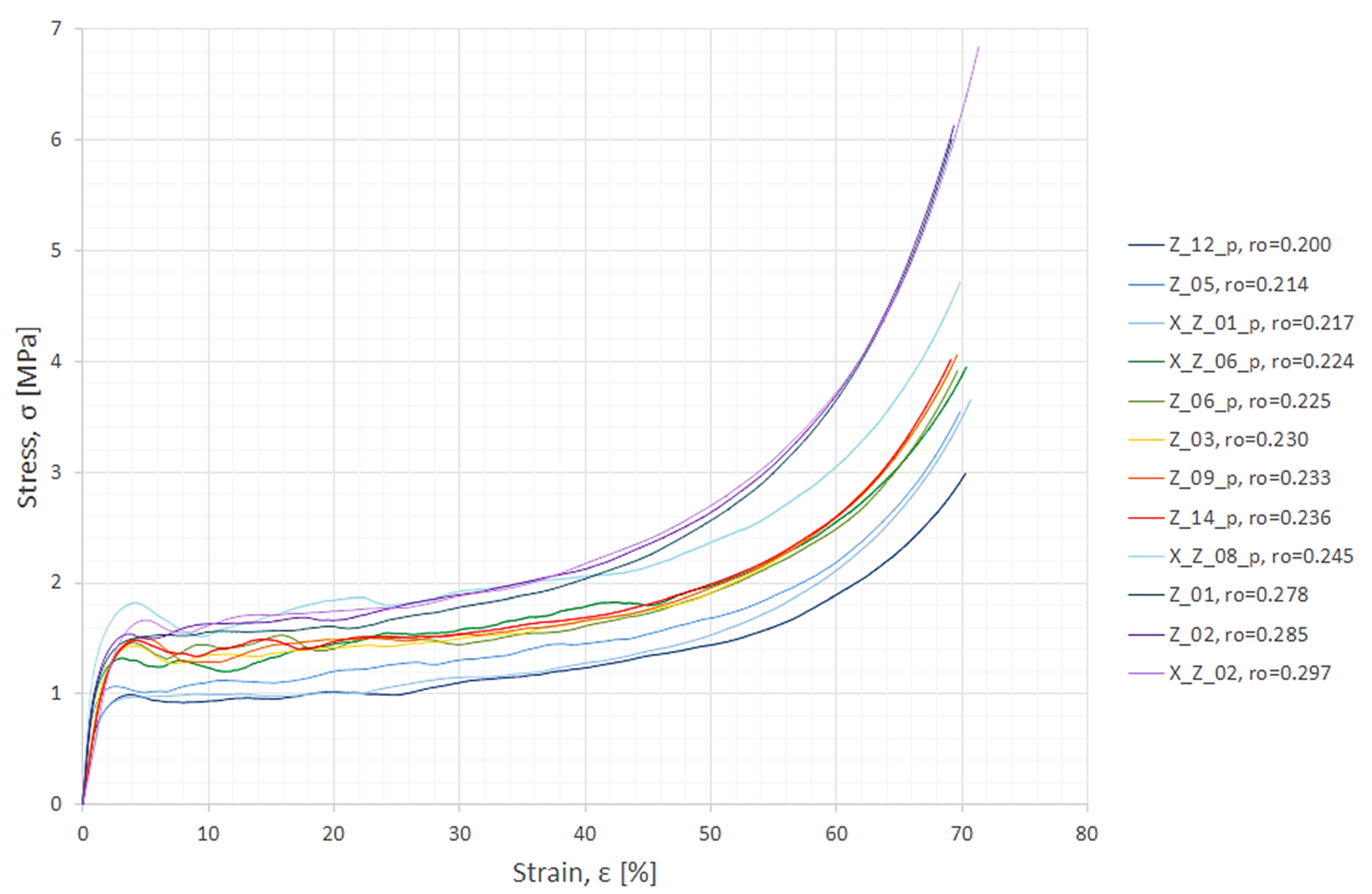
2.2. Uniaxial Compression Experiments
3. Methods: Computations with Artificial Neural Networks
3.1. Data for the Networks
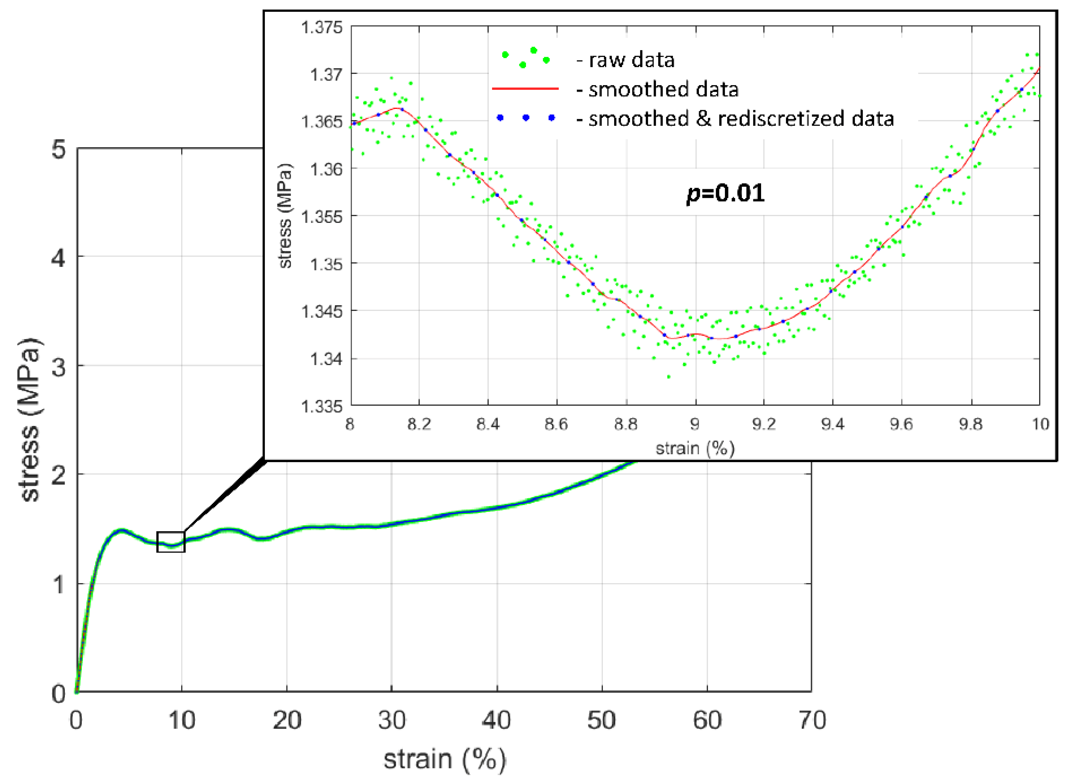
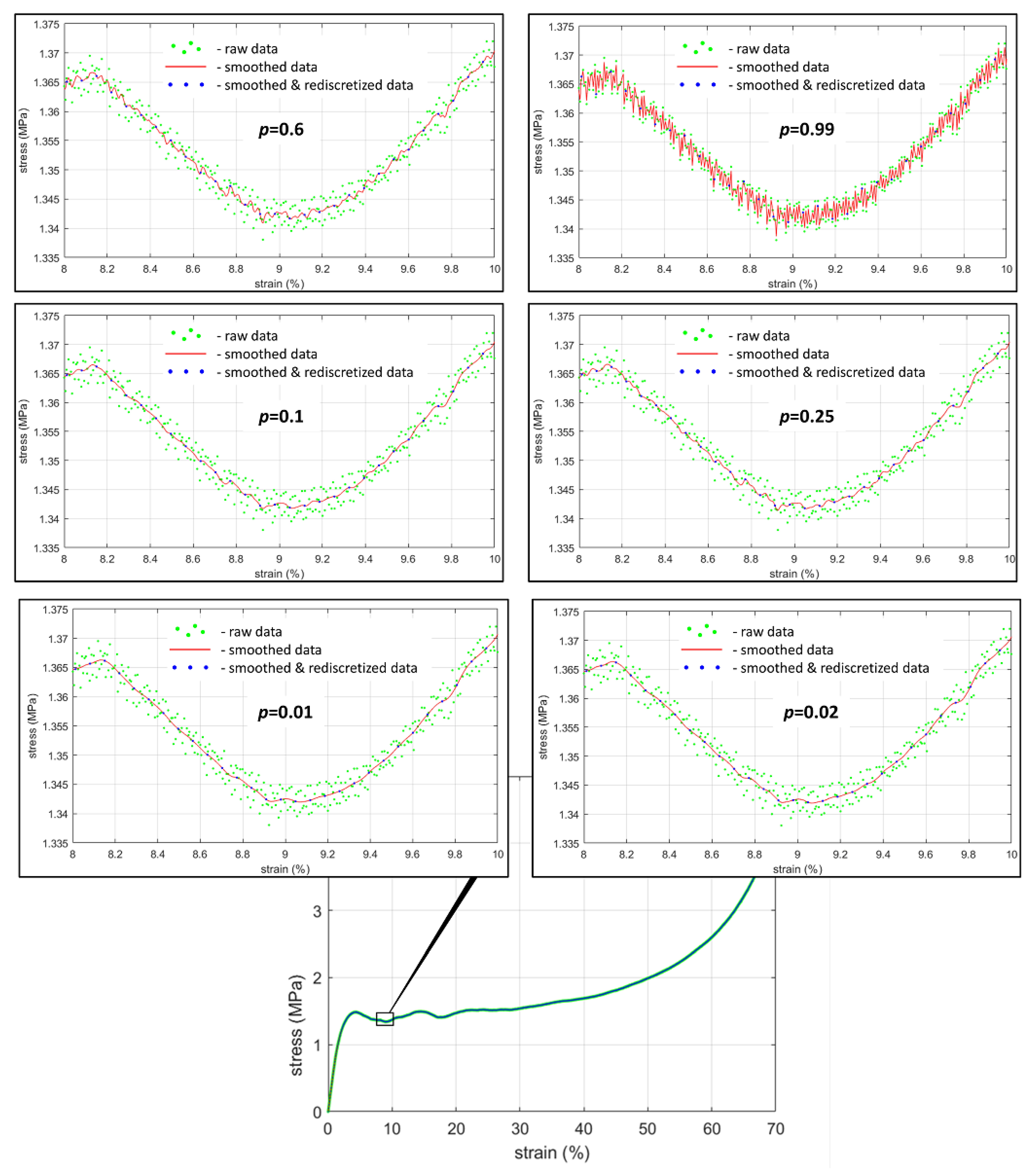
3.1.1. Initial Preprocessing of Experimental Data
3.1.2. Division of the Data Set
- Data of 11 specimens, which were devoted to building the NN model of the phenomenon of compression of these particular aluminium foam samples;
- Data of 1 specimen, which were to be used later for verification of whether the obtained model could be used as a general model, that is, for prognosing the phenomenon of the compression of aluminium foam with respect to different materials’ apparent density.
3.1.3. Normalization and Denormalization
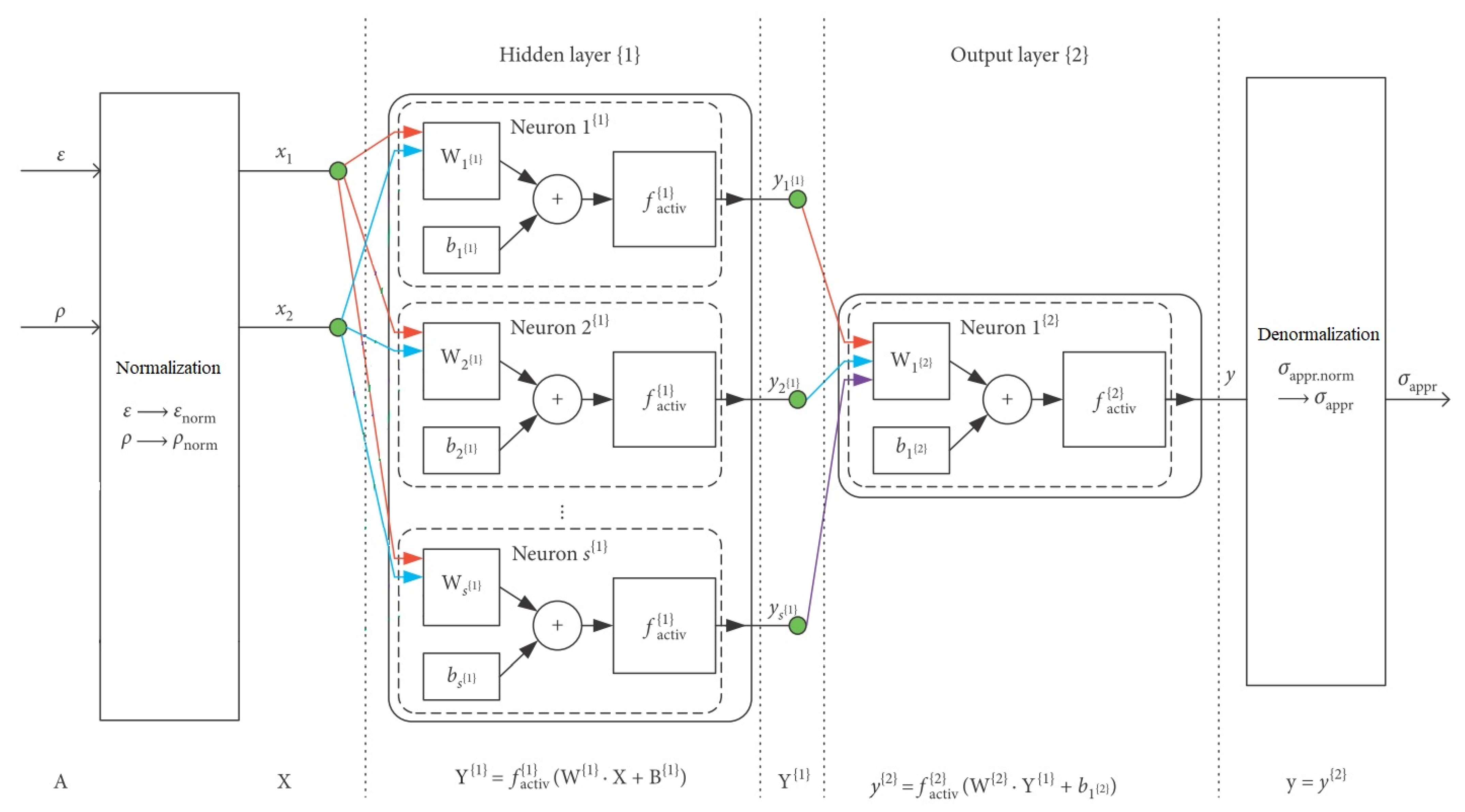
3.2. Assumed Artifitial Networks Architecture
- —the input vector, mathematically formulated as in Equation (6) below;
- —the column vector of biases for layer {1}, mathematically formulated as in Equation (7) below;
- —the matrix of weights of inputs for layer {1}, mathematically formulated as in Equation (8) below:
- —the hidden layer outputs, as in Formula (9);
- —the bias for the output layer, a scalar value;
- —the row vector of weights of inputs for layer {2}, mathematically formulated as in Equation (12) below:
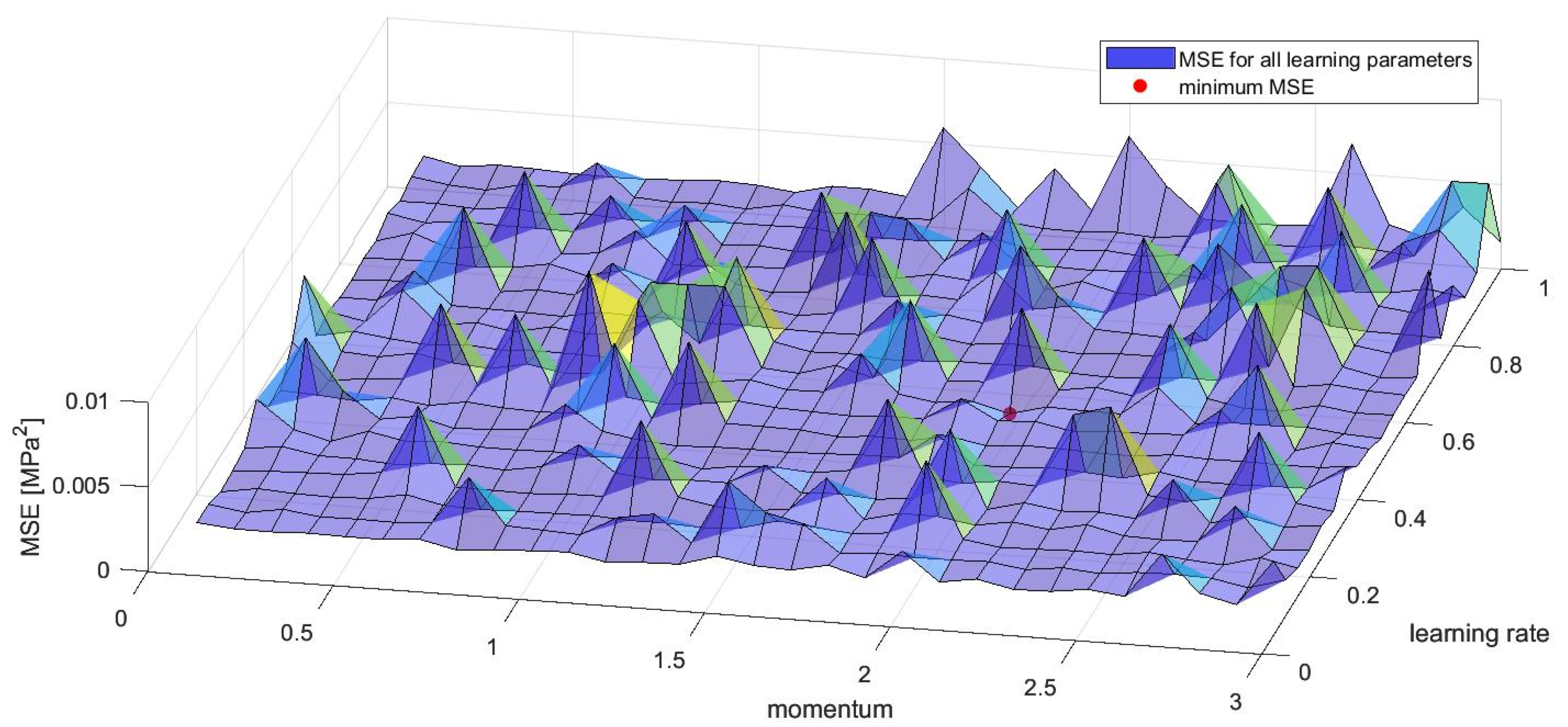
3.3. Choice of Learning Parameters
- —-th target for the network;
- —-th output for the network;
- —individual data index;
- —number of all data.
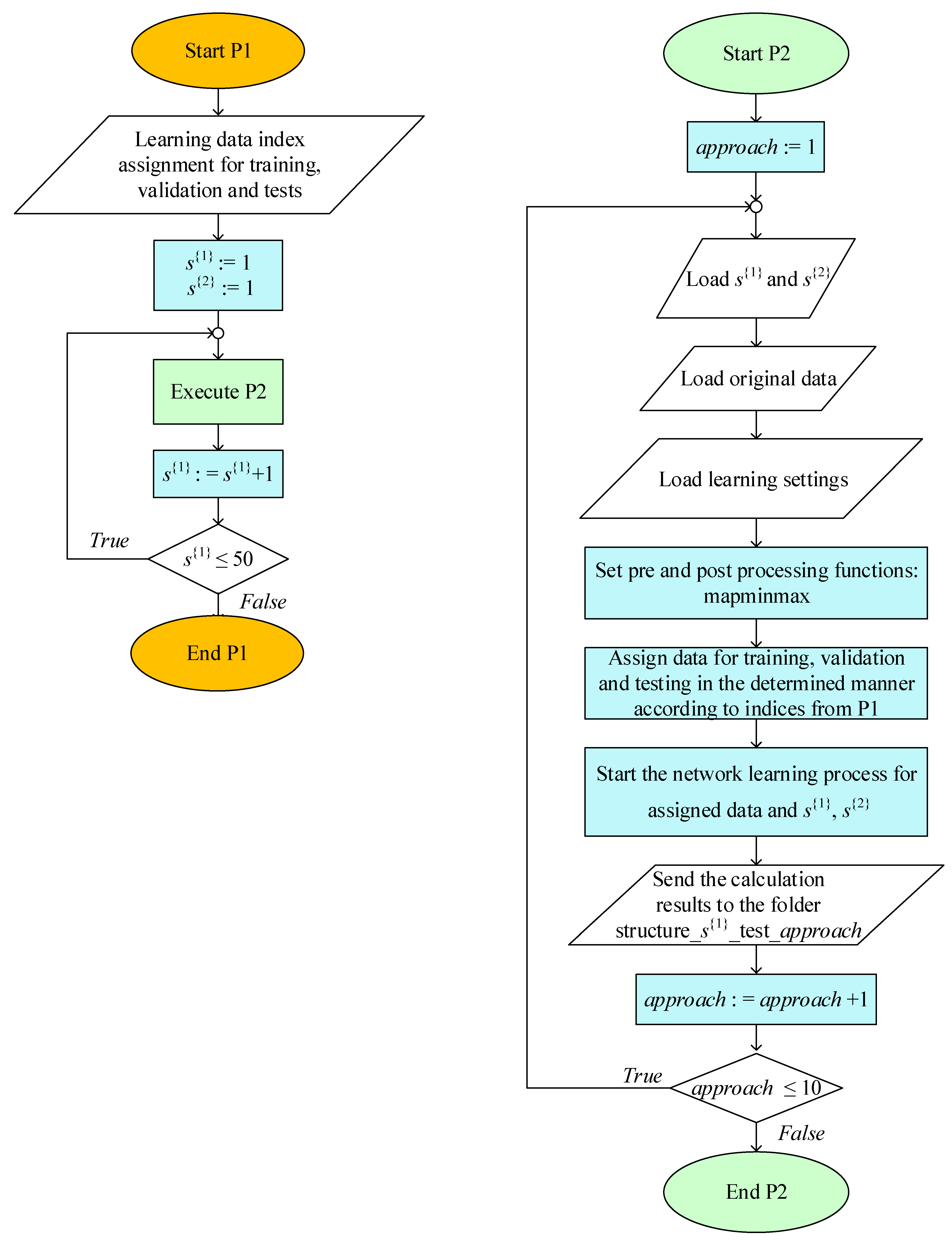
3.4. Algorithm for Building and Training Networks
3.5. Evaluation Criteria
3.5.1. The Idea of a Two-Step Evaluation
3.5.2. Accuracy of Outputs, Overfitting
- —value of the measure assumed for Criterion 1 used for the first-step evaluation;
- —given number of neurons in the hidden layer;
- —given number of repetitions of the network learning for the given network architecture;
- —maximum absolute relative error obtained for the testing stage, according to the Formula (17):
- —-th target for the network in the testing stage;
- —-th output for the network in the testing stage;
- —individual data index, should exhaust all data.
- —value of the measure assumed for Criterion 1 used for the second-step evaluation;
- —mean absolute relative error from the verification of the network with the given and taught in the given against external data;
- —threshold for Criterion 1 used for the second-step evaluation;
3.5.3. Speed of Calculations
- —value of the measure assumed for Criterion 2 used for the first-step evaluation;
- —threshold for Criterion 2 used for the first-step evaluation;
- , and —defined as in Formulas (16) and (17).
- —value of the measure assumed for Criterion 2 used for the second-step evaluation;
- —mean absolute relative error from the verification of the network with the given and taught in the given against external data;
- —threshold for Criterion 2 used for the second-step evaluation.
3.5.4. Robustness
- —value of the measure assumed for Criterion 3;
- —total number of for the given ;
- —threshold for Criterion 3;
- —as in Formula (24):where remaining symbols are denoted as in (14,15).
- —value of the measure assumed for Alternative Criterion 3;
- —threshold for Alternative Criterion 3, which may also not necessarily be assumed as 0;
- —number or percentage value for total that must comply with Condition (26);
- other symbols—as defined in (23).
4. Results and Discussion
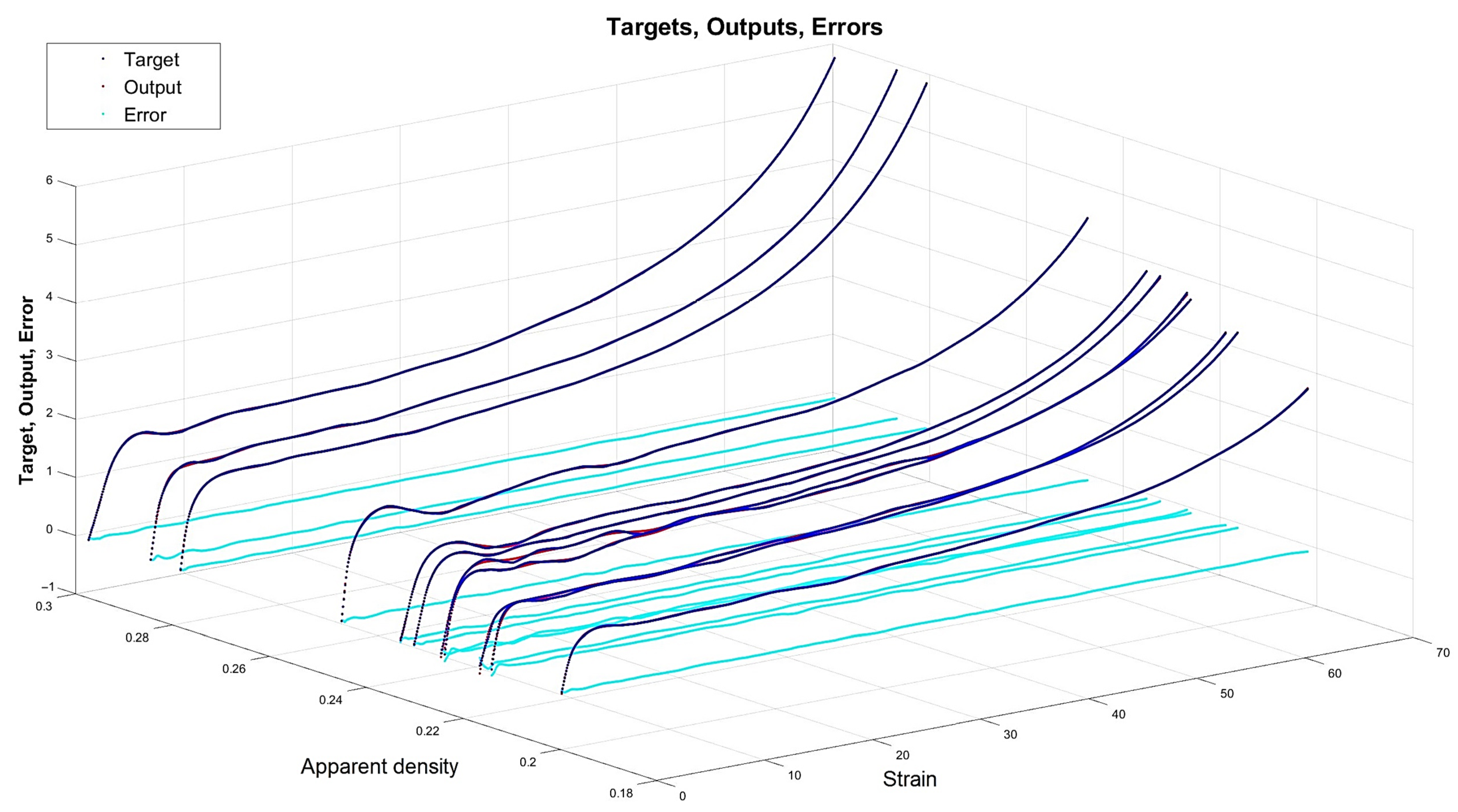
- Section 4.1 will give results from the validation stage from the training of networks (11 sample data set).
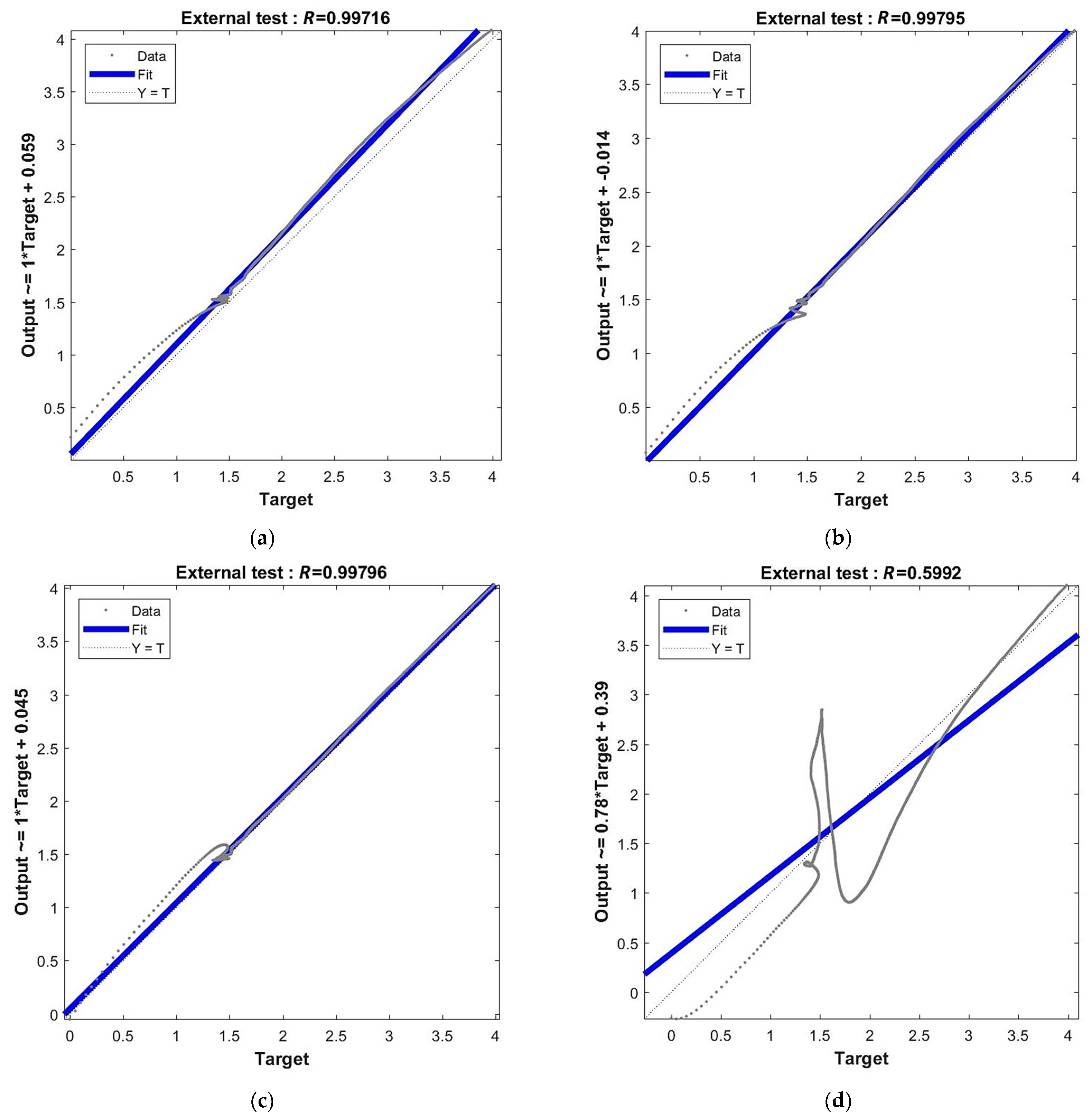
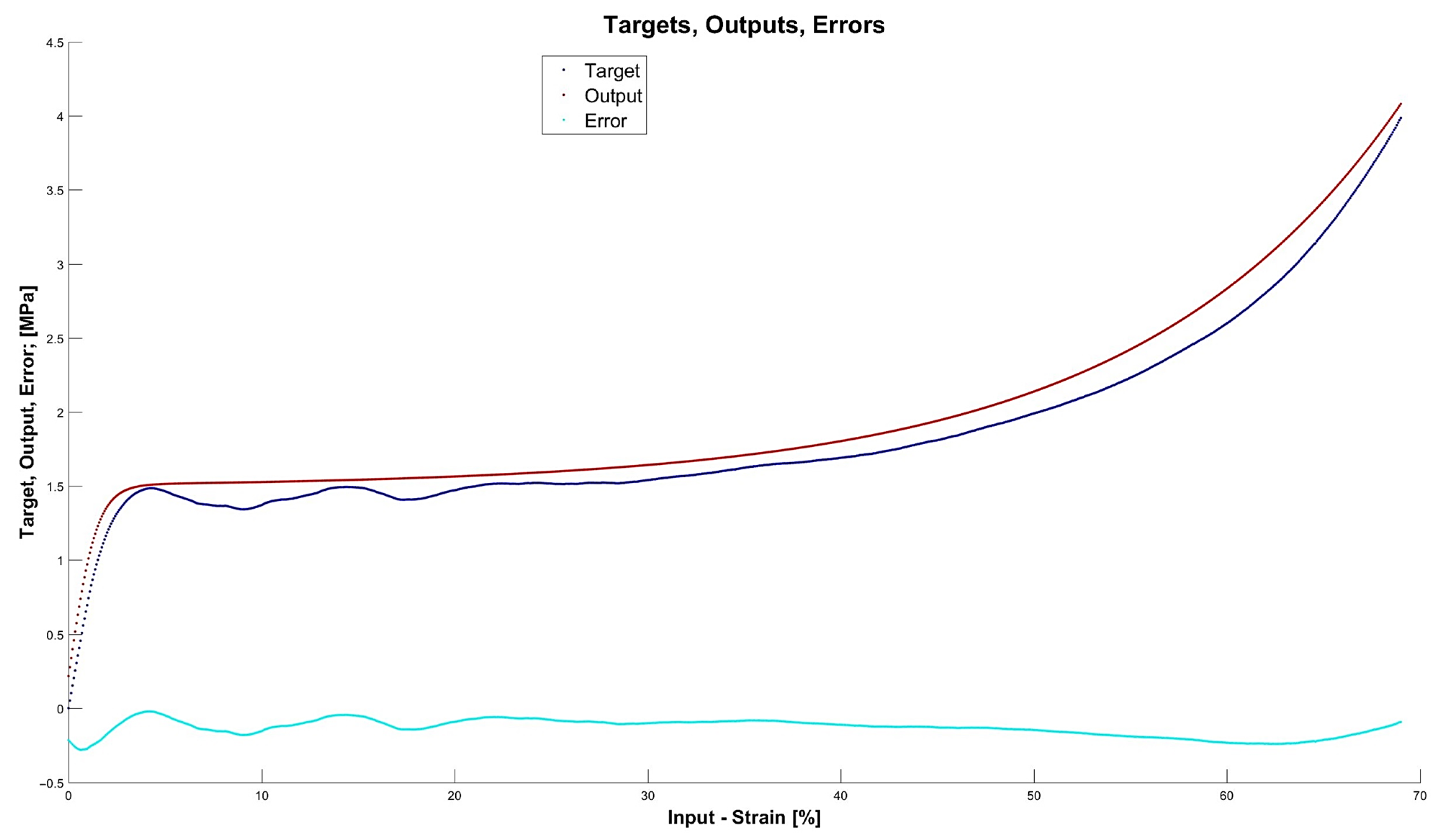
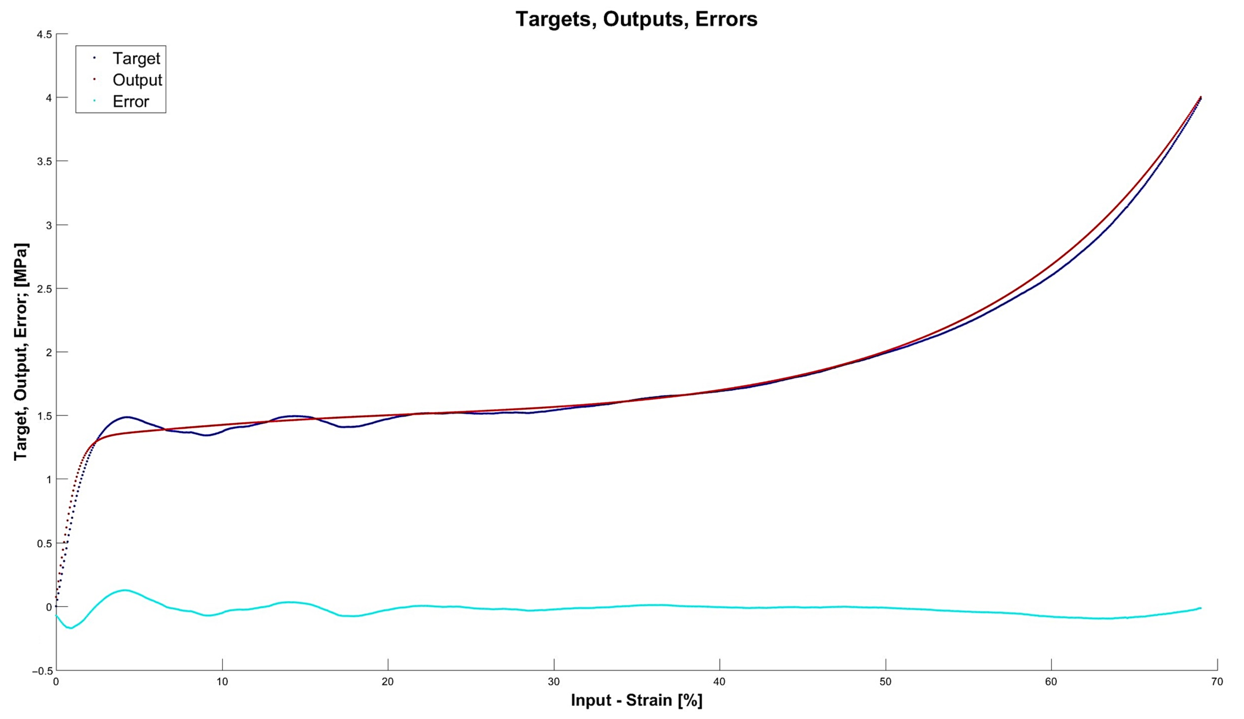
- Section 4.2 will be devoted to choosing the most adequate network according to criteria of the first- and second-step evaluation and thus will show results from the test stage of teaching networks (11 sample data set) as well as from the verification of networks against external data (specimen Z_14_p).
- Section 4.3 will present detailed results for the final chosen networks.
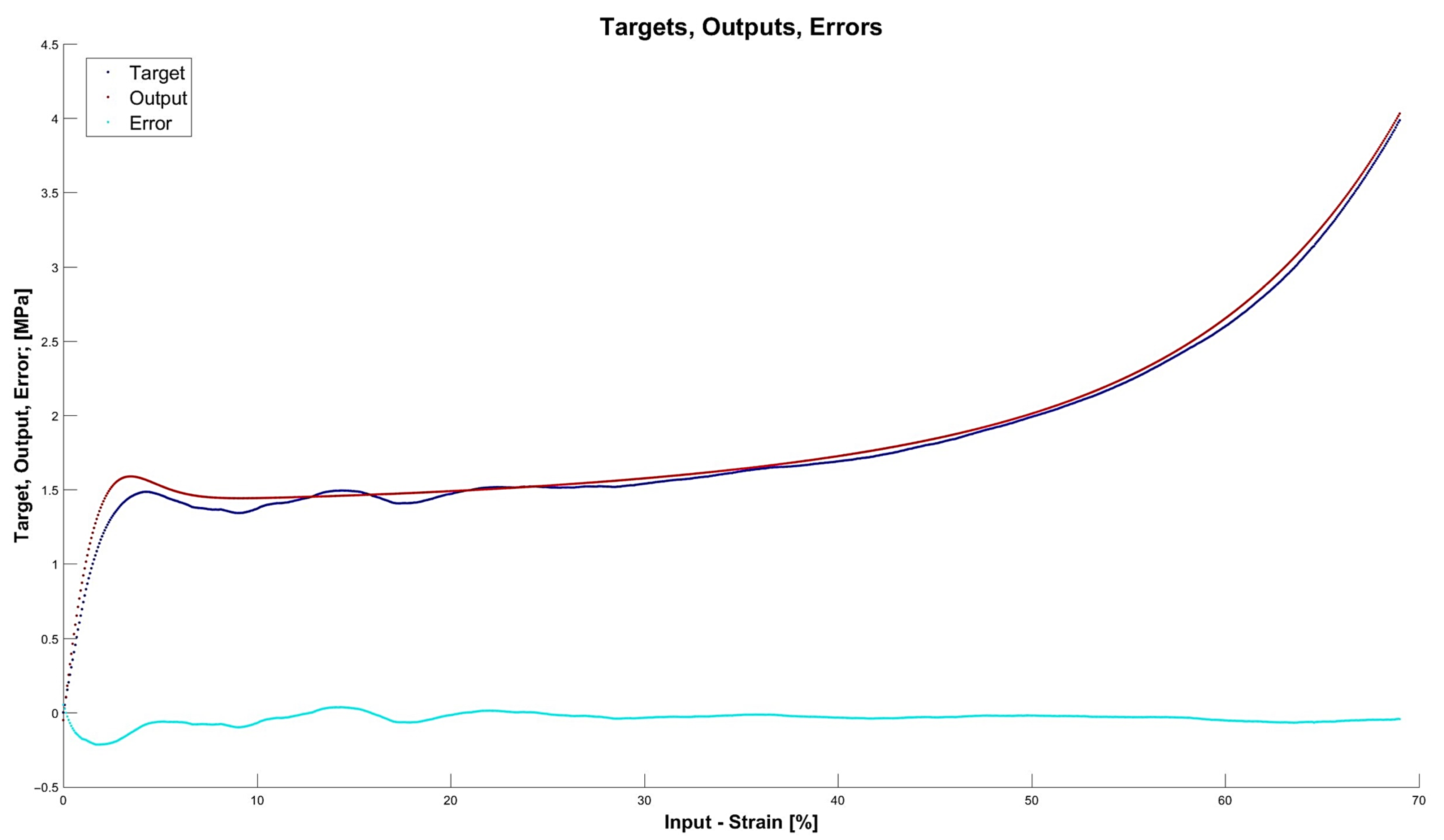
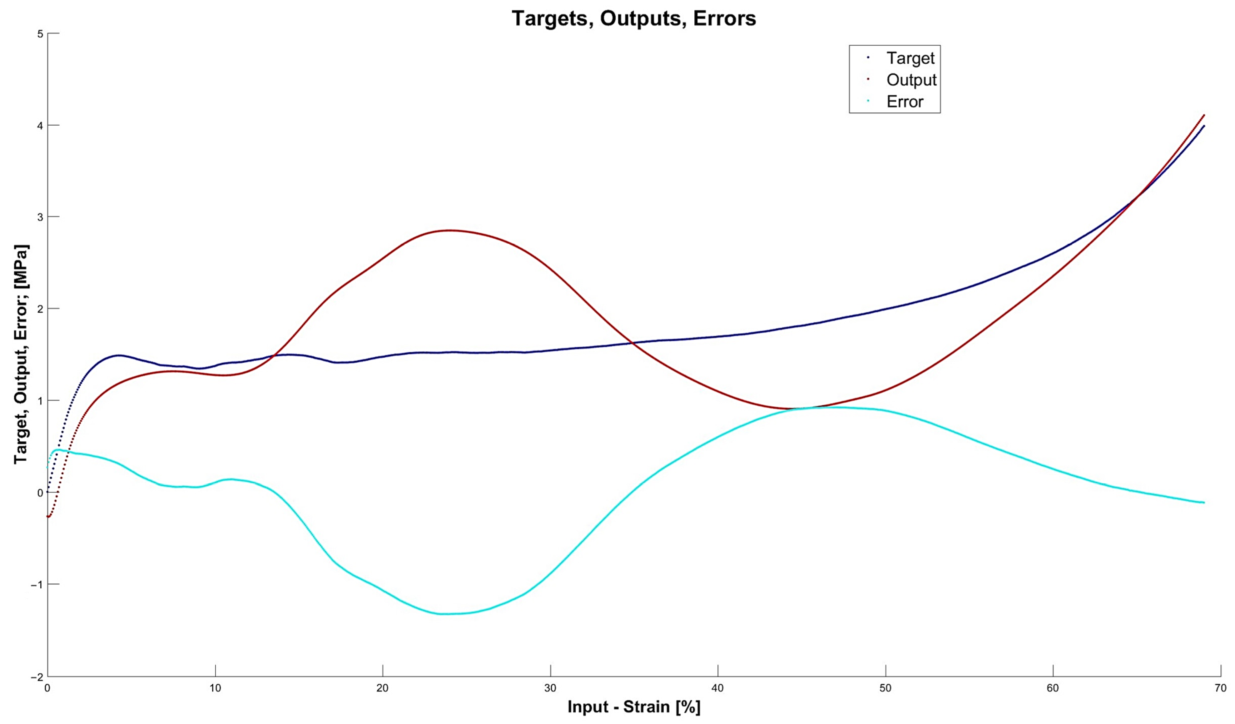
4.1. Internal Network Evaluation and Robustness
4.2. Choice of the Most Appropriate Network Specifications
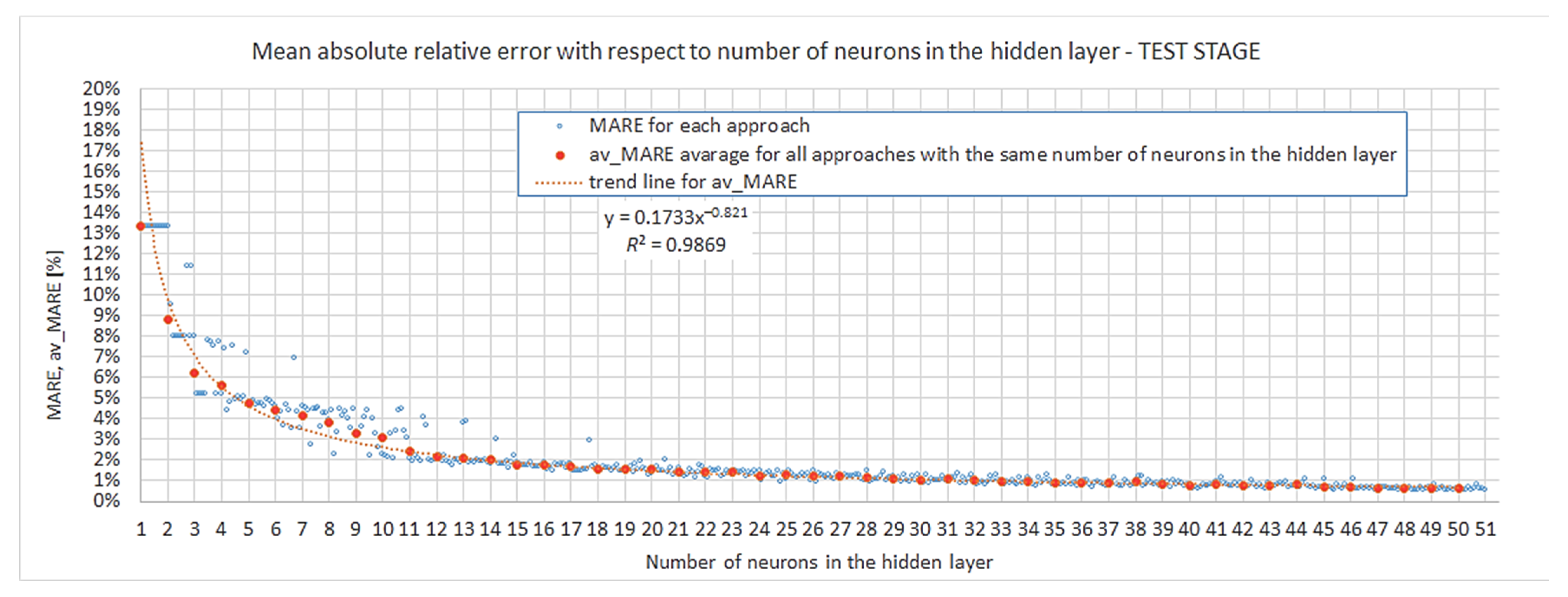
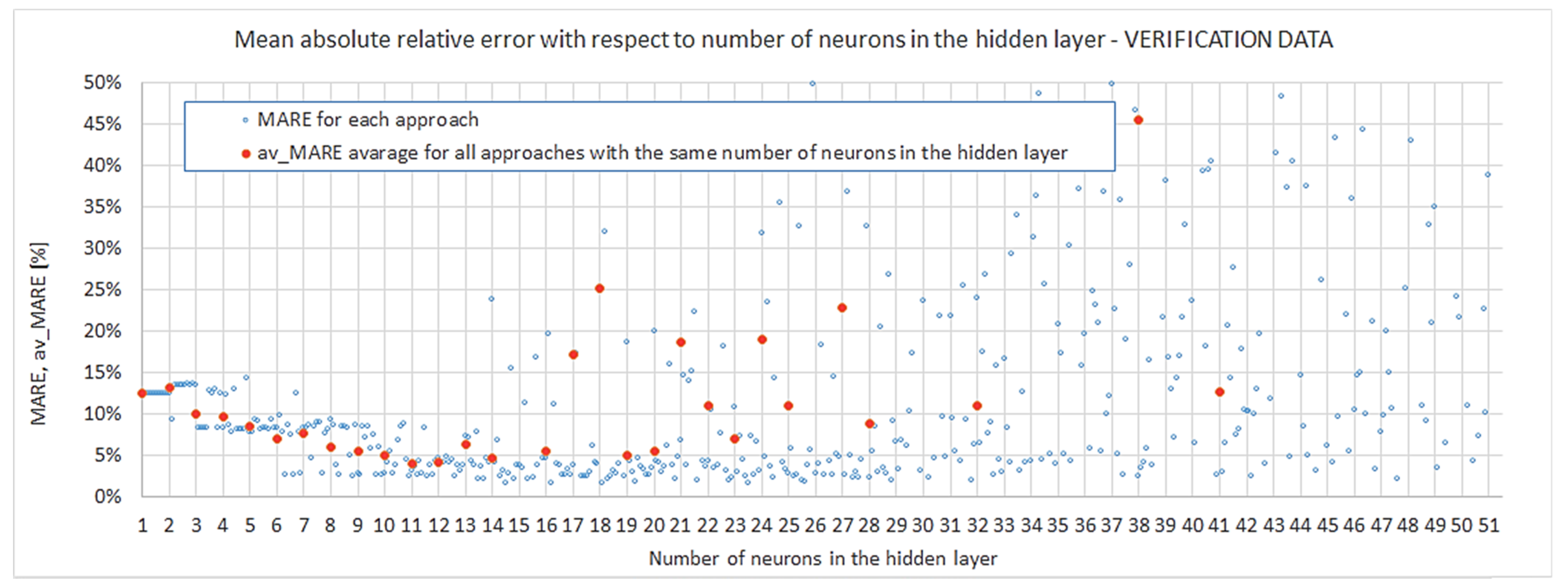
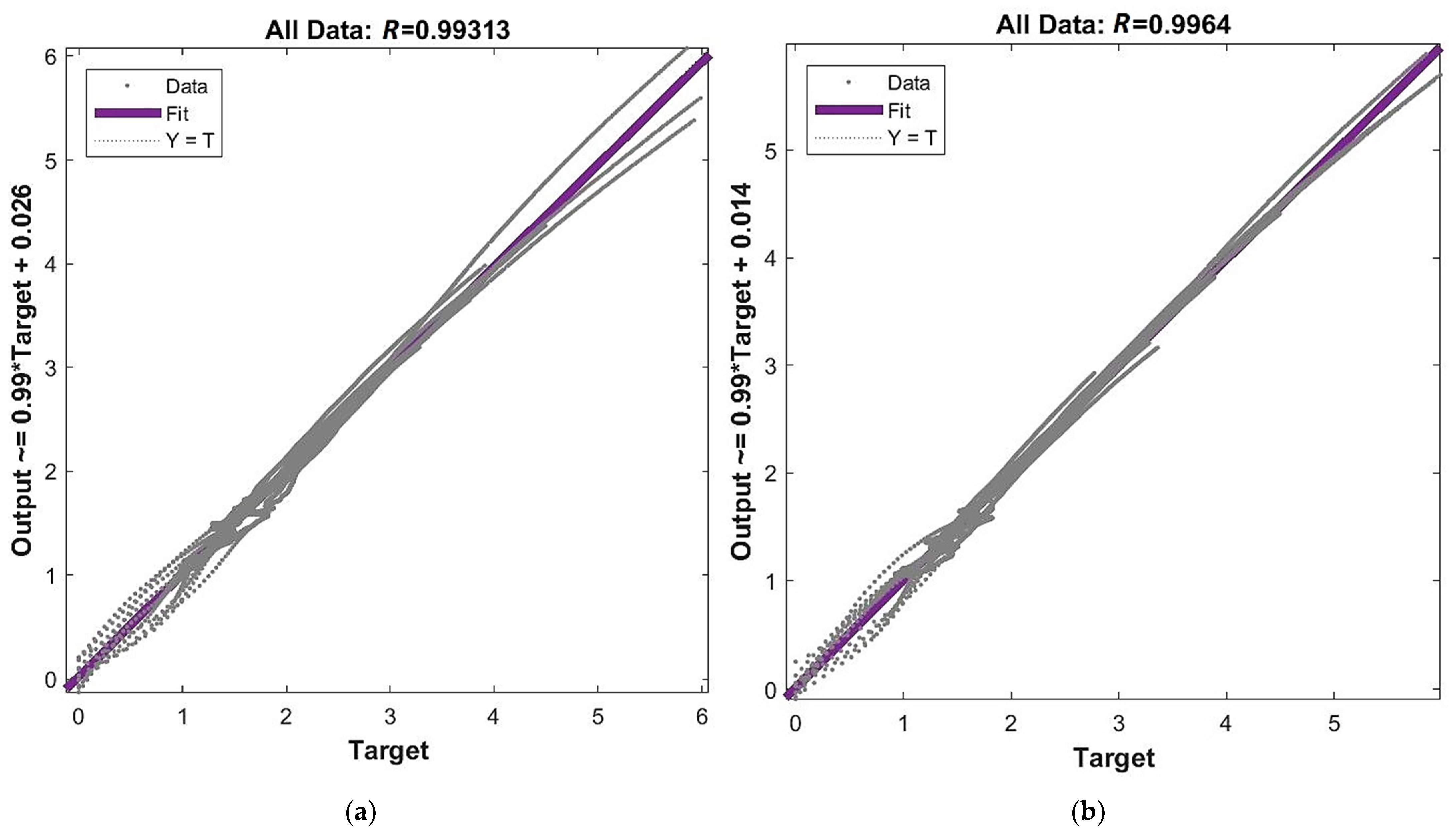
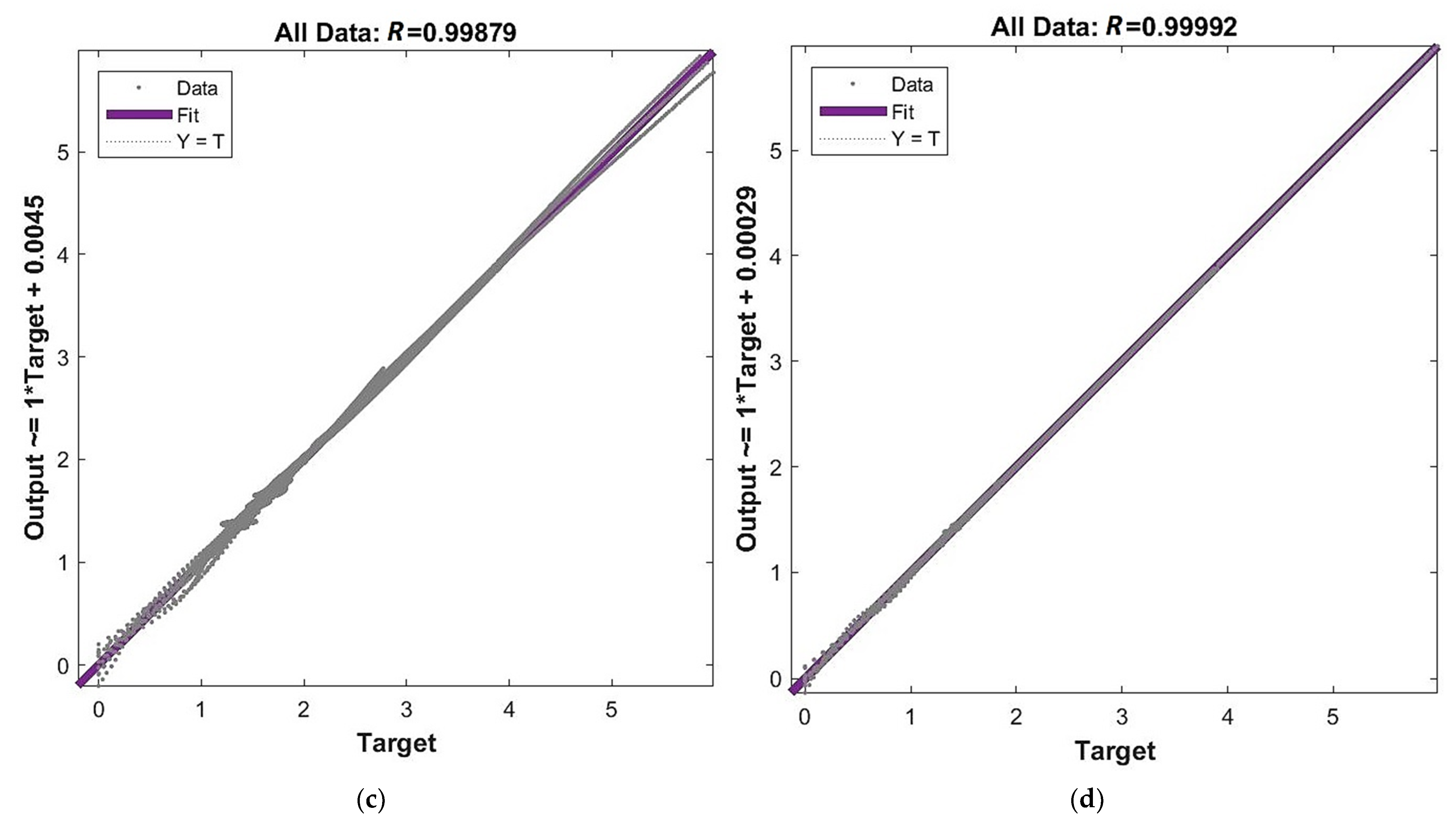
4.2.1. Most Accurate Outputs, Overfitting
4.2.2. Outputs in Terms of Increasing Speed of Calculations
- —given fixed number of neurons in the hidden layer;
- —total number of for the given ; here
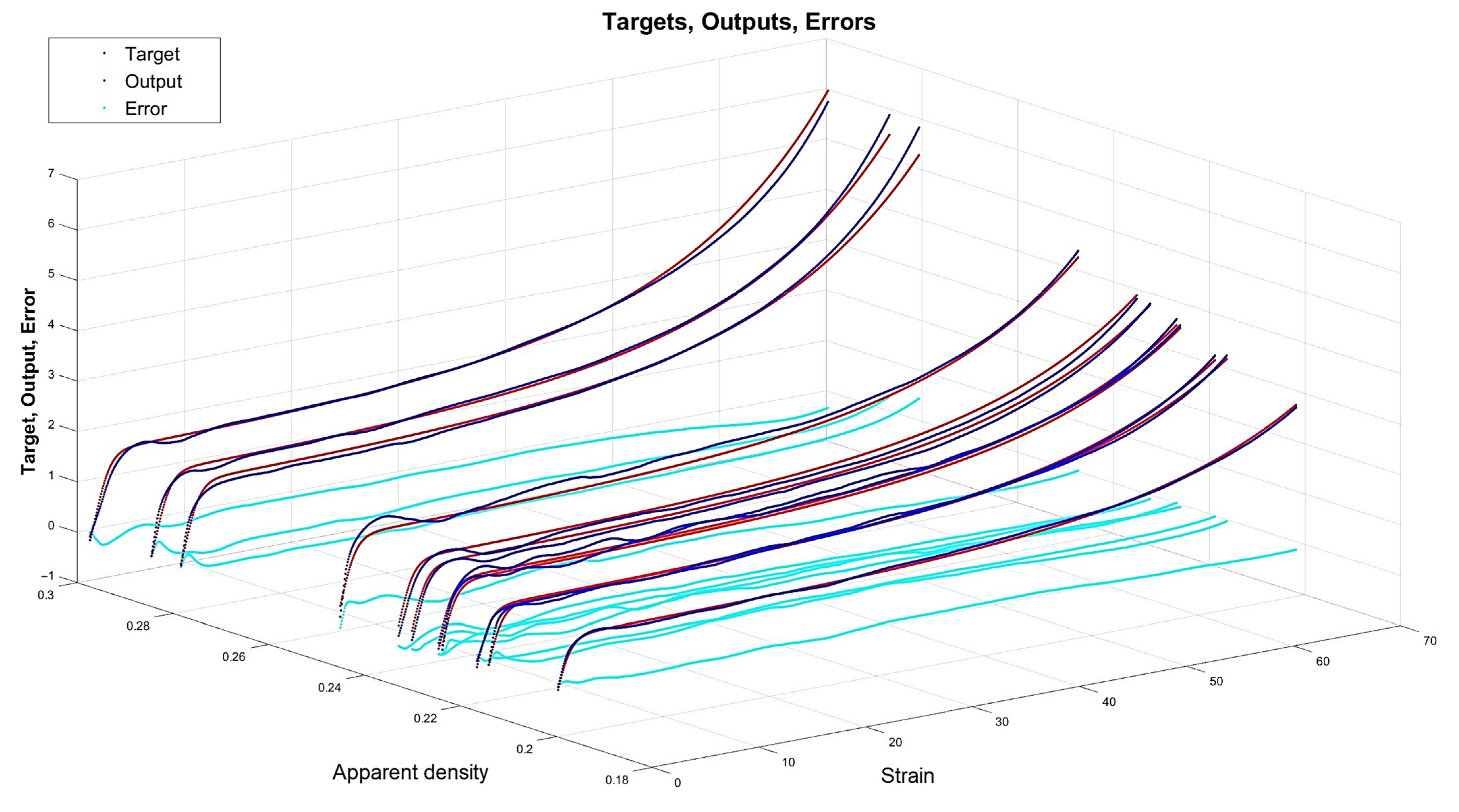
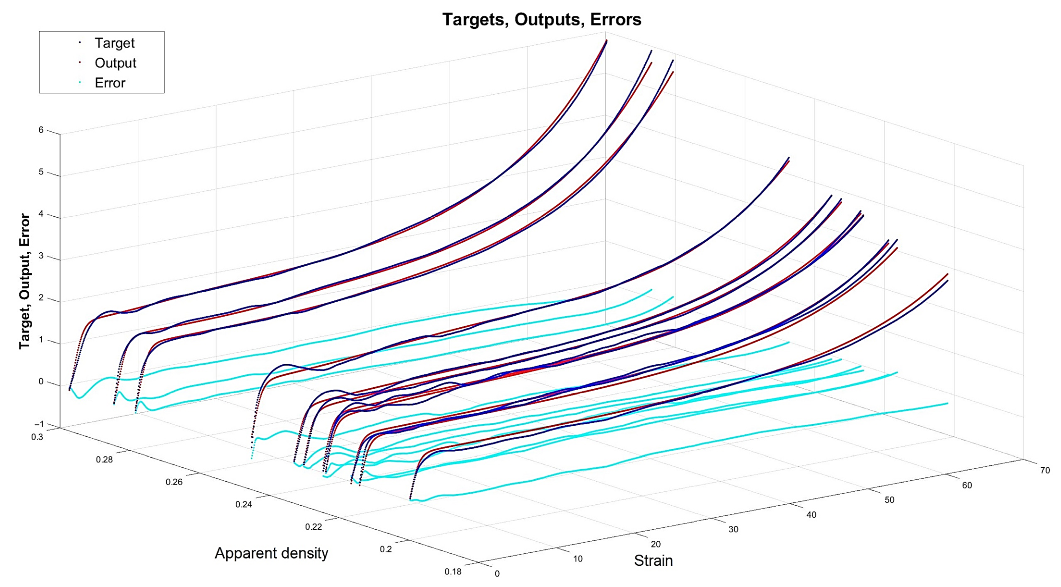
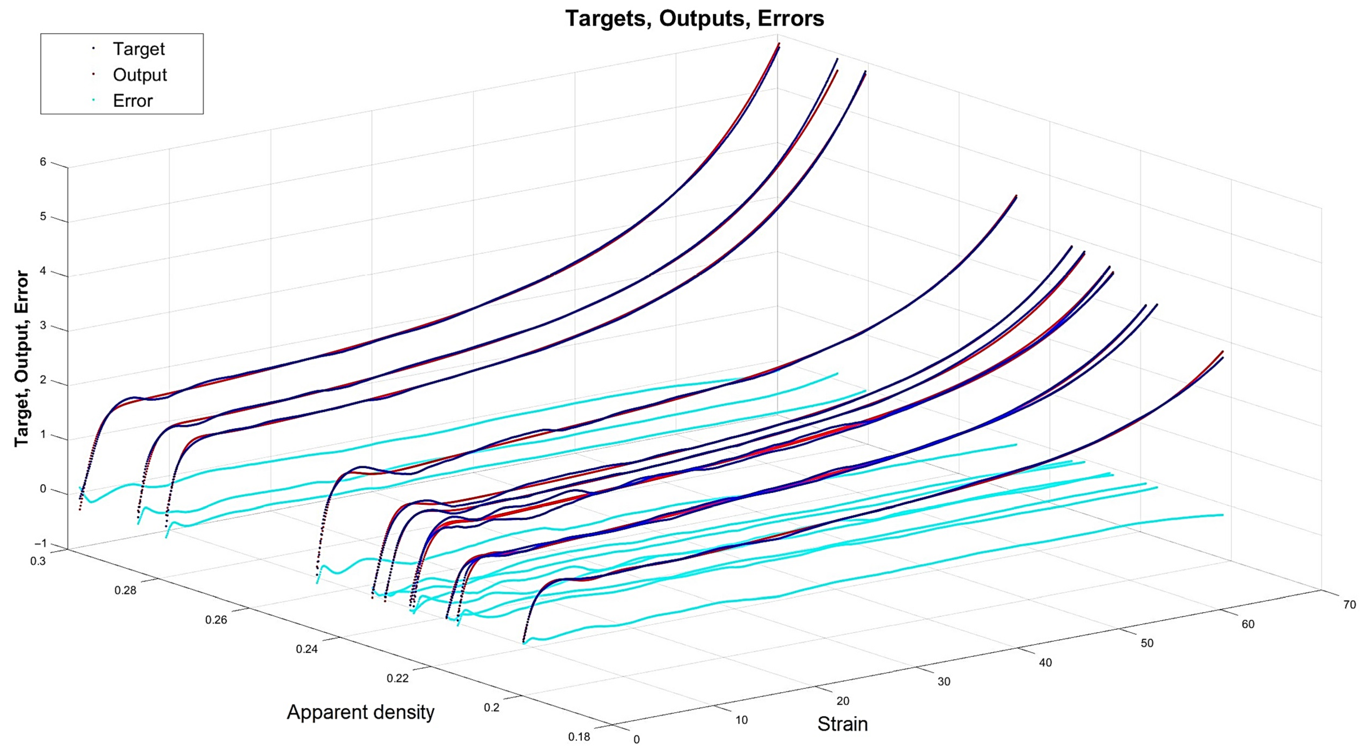
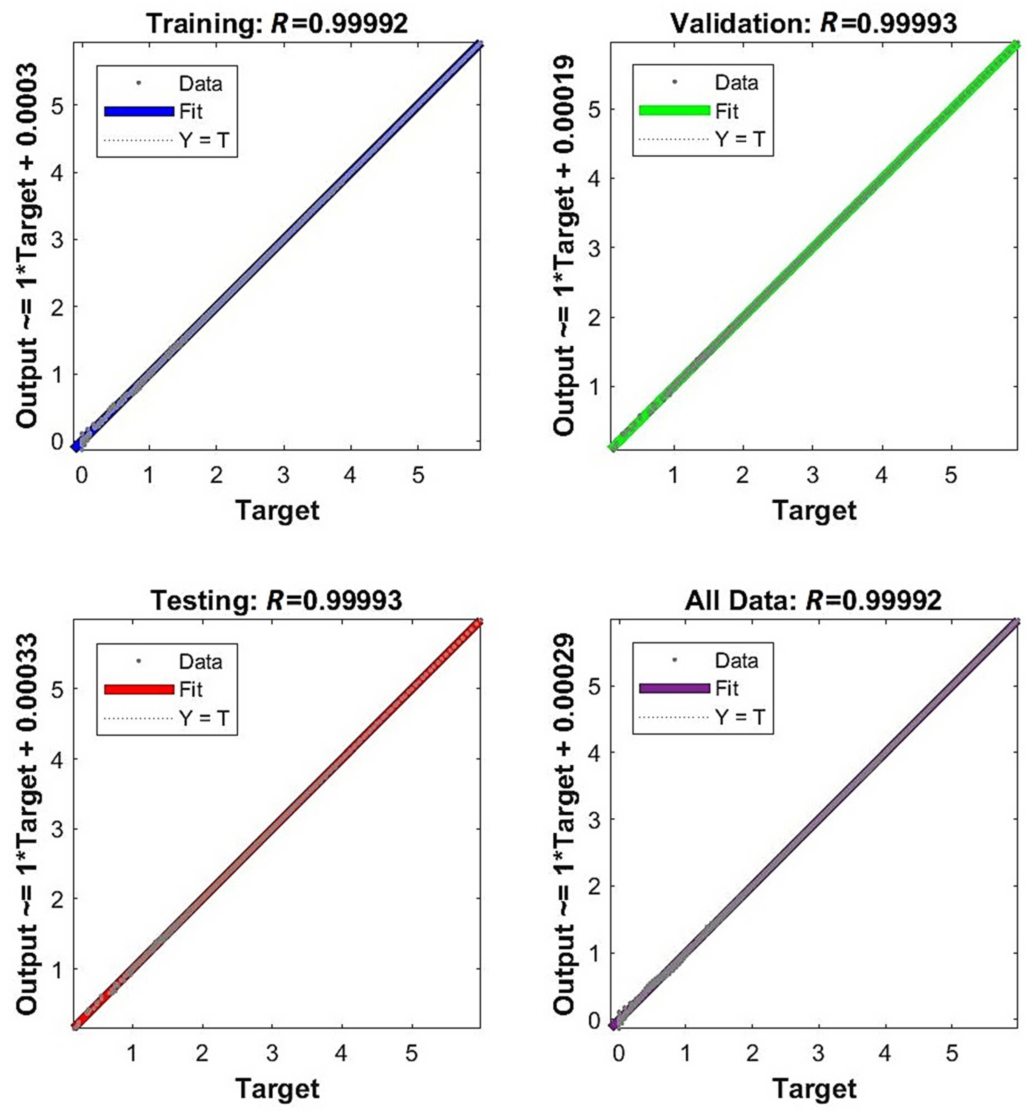
4.3. Results for Optimal Networks
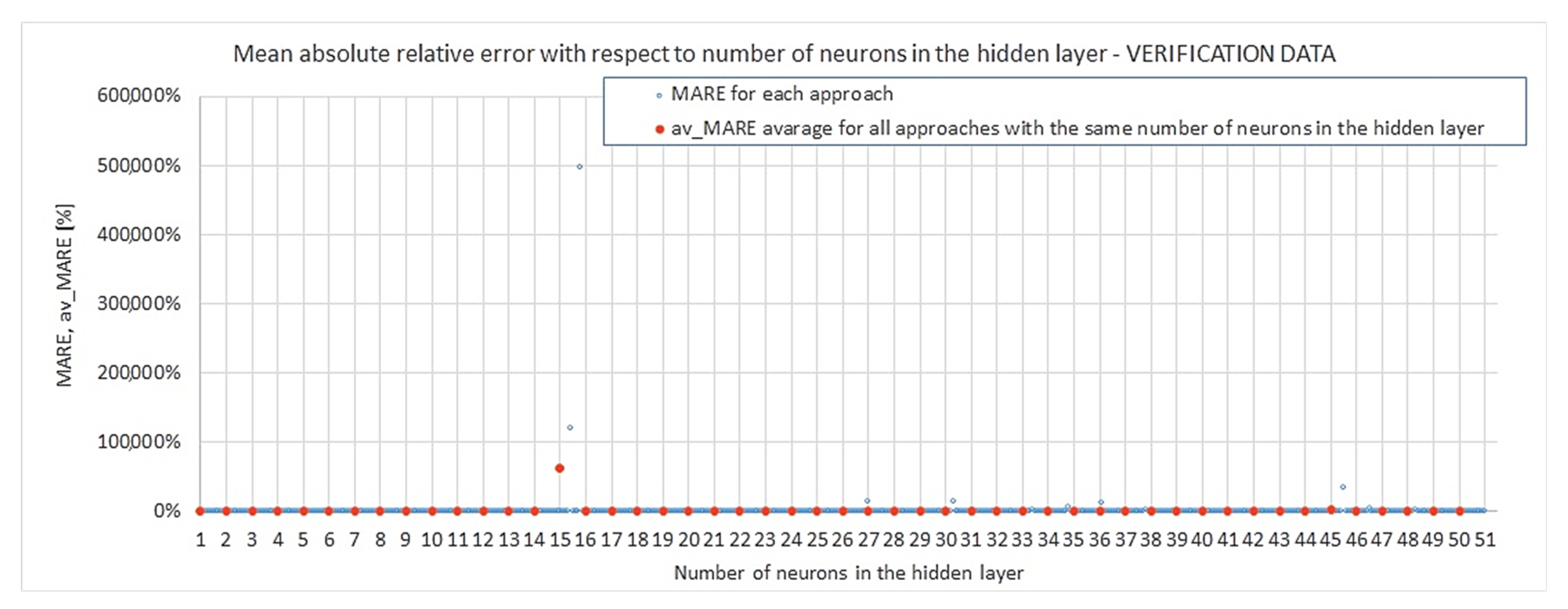
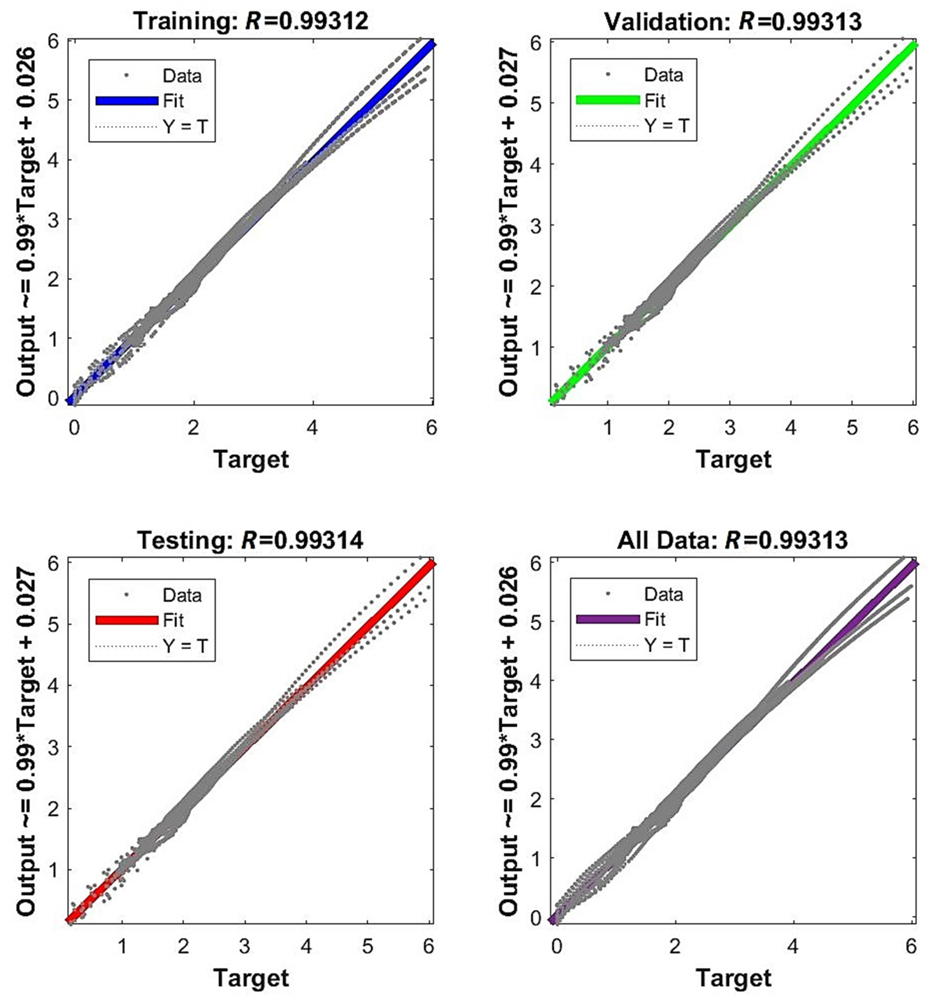
- The network is the least complex structure, but still provides acceptable accuracy itself and for prognosis ; however, four neurons do not guarantee robustness.
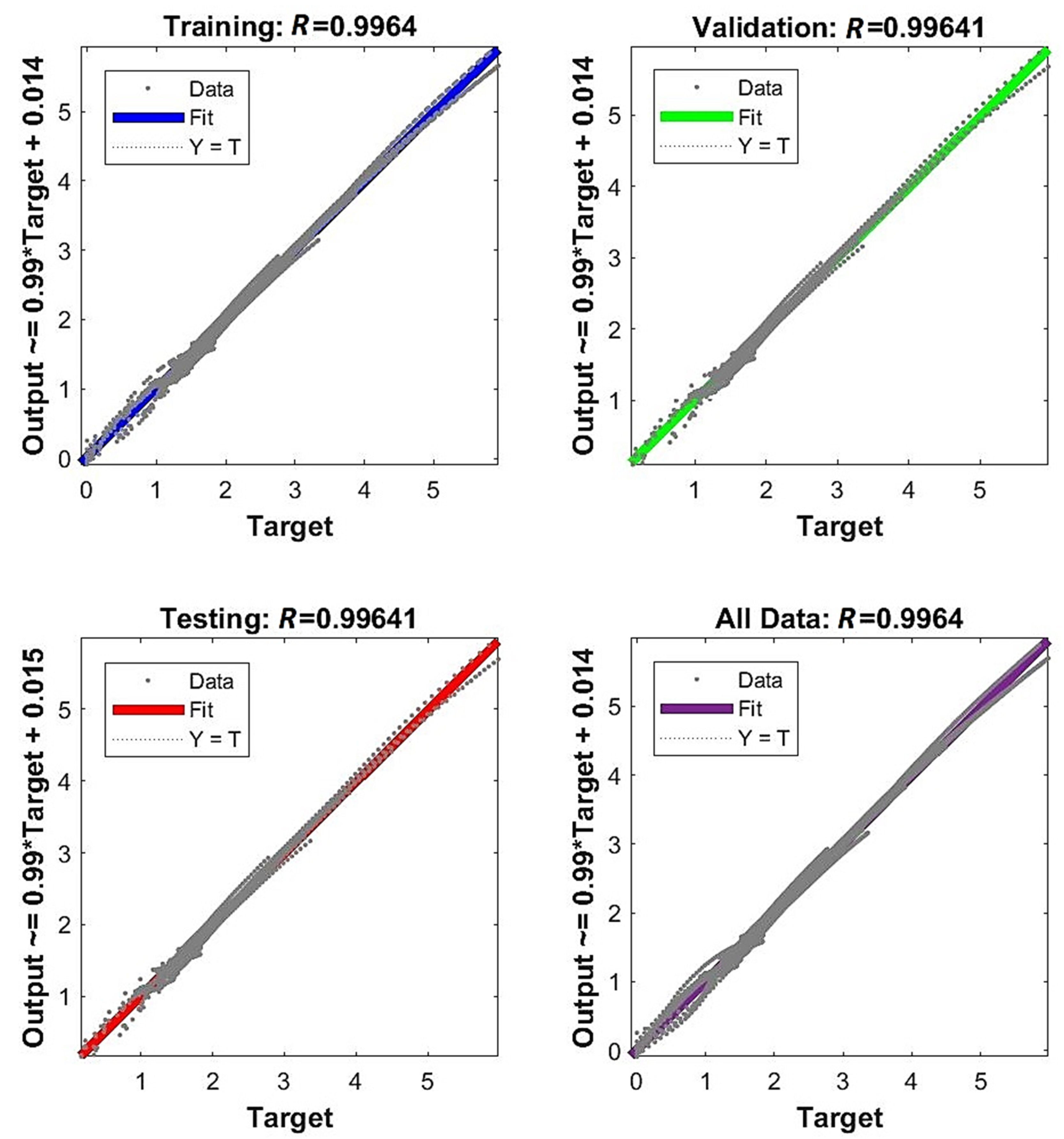
- The network is still a relatively simple structure but assures good accuracy itself and for prognosis ; but six neurons do not guarantee robustness.
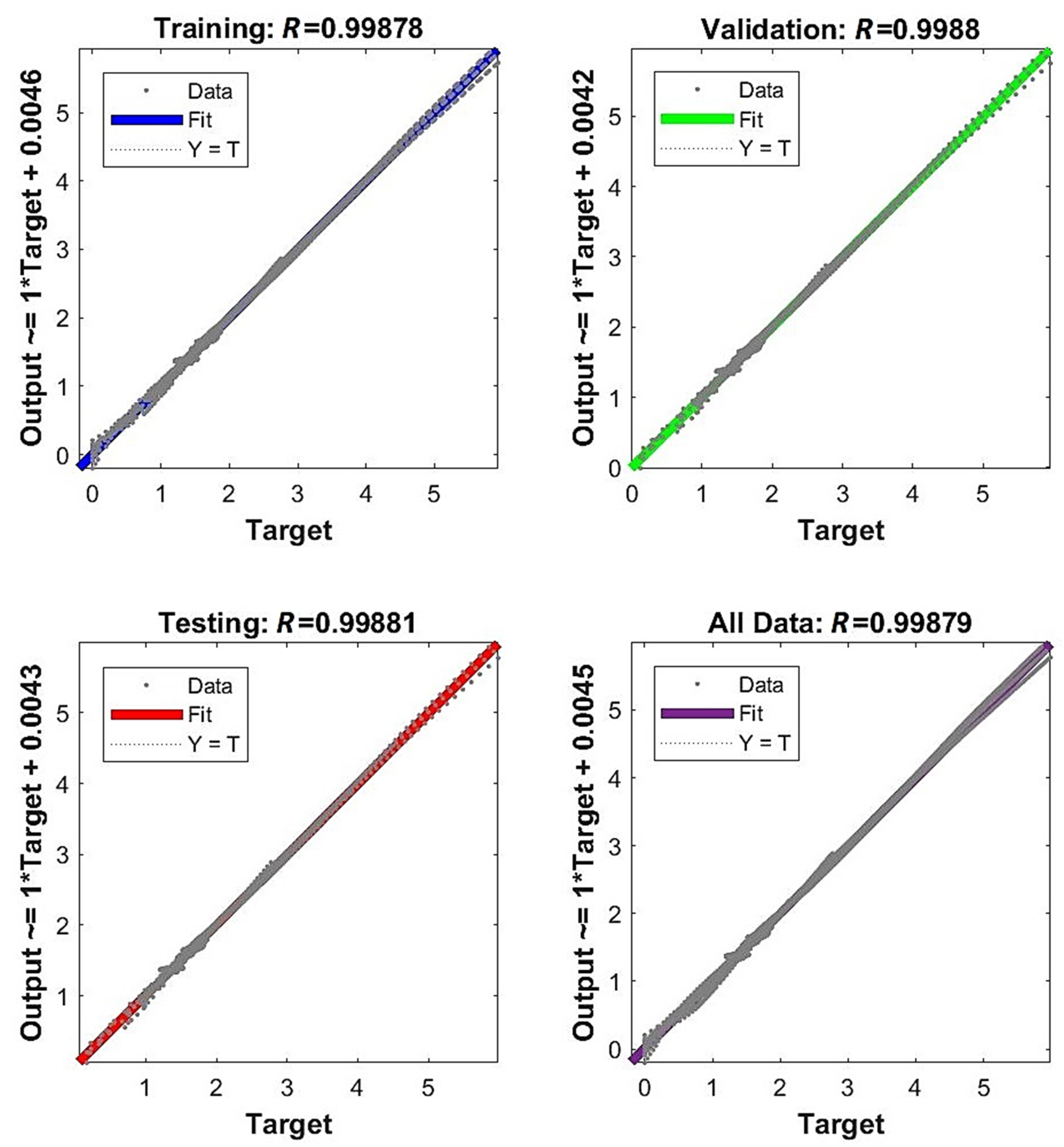
- The network is a relatively complex structure; however, it shows very good accuracy on many levels, including and for prognosis ; also, 11 neurons are within the boundary of 80% robustness.
- The network is a very complex structure, showing extremely good particular accuracy and very adverse overfitting in prognosis ; 48 neurons are very safe in terms of robustness.
5. Conclusions
- The following neural network architecture specifications can be successfully used to model the addressed phenomenon: a two-layer feedforward NN with one hidden layer and one output layer. As for the activation functions, one may use the hyperbolic tangent sigmoid function in the hidden layer and the linear activation function for the output layer. As for the training algorithm, the Levenberg–Marquardt procedure was verified positively. For this procedure, the mean square error was used as the performance function with 0 as its goal. The learning rate and momentum should be calibrated; however, for the given experimental data and the number of neurons in the hidden layer assumed as 12 (near optimum) the results show that the influence of these two parameters was not the deciding factor. Values for momentum, learning rate, number of epochs to train, gradient and maximum validation failures, which were applied and recommended, are given in Table 2.
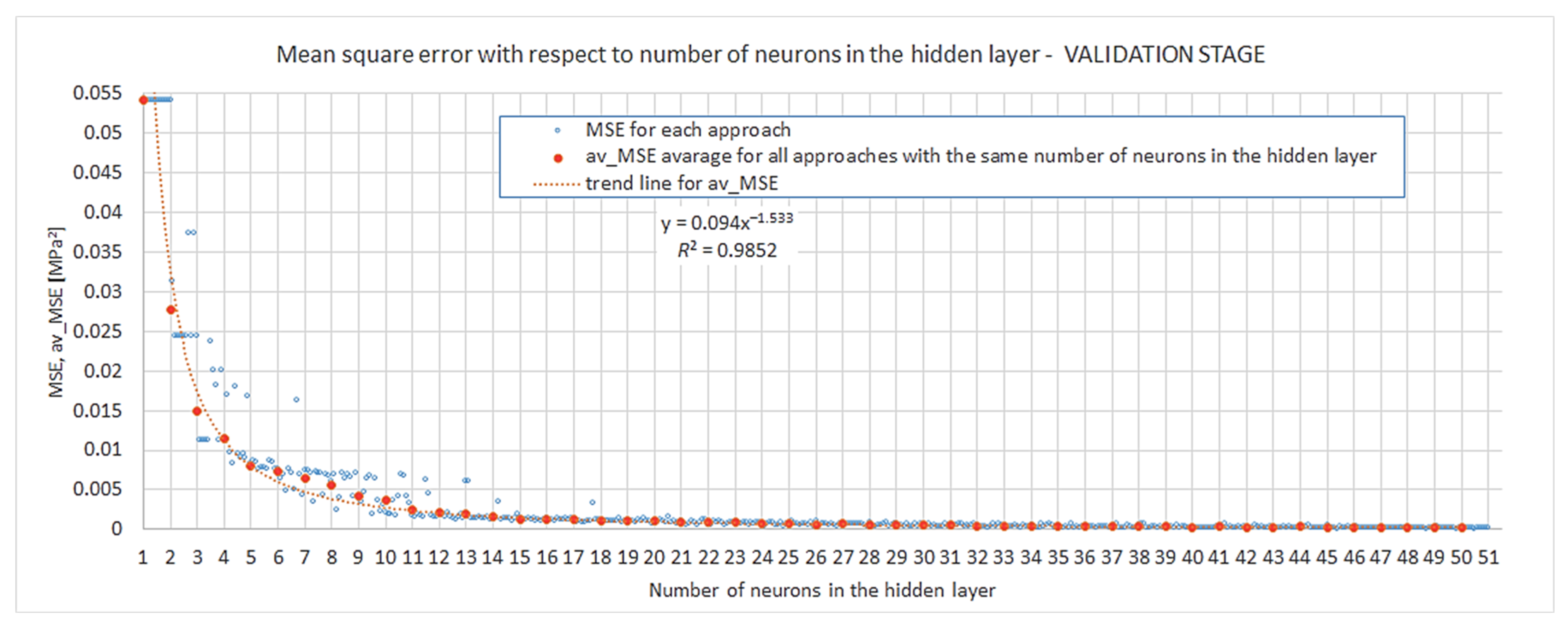
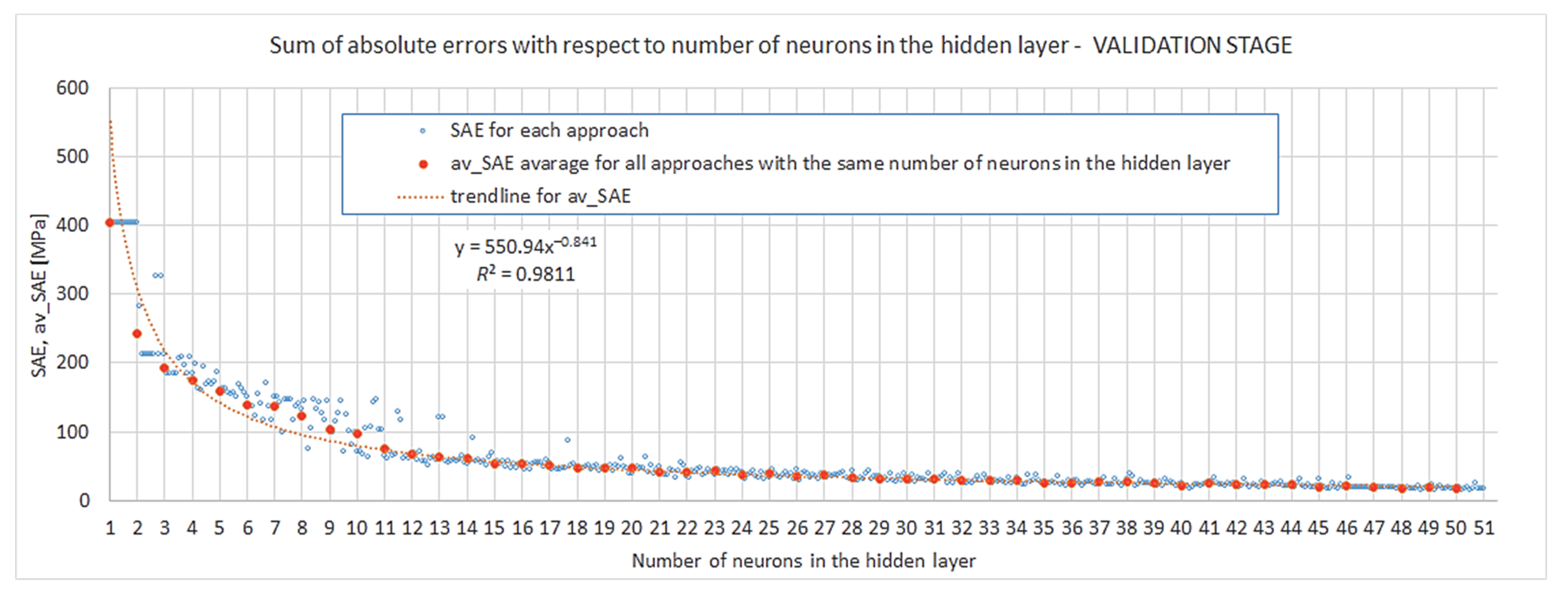
- Regarding the number of neurons in the hidden layer, the interval was investigated. It was shown that even a relatively low complexity of four neurons can provide a satisfactory particular model and acceptable accuracy for the prognosis (, ); nevertheless, the probability of obtaining such results by the first approach of training a model is low. Increasing the complexity by two neurons—up to six—considerably improves the accuracy of a particular model itself and prognosis (, ); however, robustness is not satisfied for such networks. If one is interested in complying with insensitivity in the random assumption of weights and biases, networks with 11 neurons in the hidden layer provide robustness with a probability of 0.8 and a very good accuracy level at the same time (, ). A greater number of neurons in the hidden layer () also gives accurate results, but the accuracy is not increased substantially, and the overfitting risk is higher with 13 neurons or more.
- In order to choose the model which most appropriately prognoses the mechanical characteristics of the studied materials, it is necessary to consider certain statistical measures for the assessment of the obtained results. In particular, evaluation parameters which indicate the occurrence of single instants of significant deviations between a mapped value and the respective target (e.g., MaxARE) should be introduced. Such individual considerable errors might disqualify a given model even if overall mean error would be on satisfactory level (for example MARE, MSE).
- A series of criteria (16)–(26) is proposed to evaluate obtained models in a two-step evaluation. The idea of the two-step verification allows one to assess the fitting of the particular model to the data with which it was trained and to assess whether this particular model is capable of prognosing. Based on the presented research, it is recommended that the two-step model evaluation is performed with regard to the following qualities and measures explained in Section 3.5: accuracy (, ), under- and overfitting (, , , ) and robustness ().
- The relationship between the number of neurons in the hidden layer and convergence (meant as nearing to ) can be very well described by a power law, which proves that the modelling of closed-cell aluminium during compression is not a chaotic but ordered phenomenon. However, at the same time the results show that for networks with 13 neurons and more, instances burdened with considerable overfitting start to occur. These two facts may indicate that in the pursuit of better accuracy, instead of increasing the number of neurons in the hidden layer {1}, one may choose to lower it while also adding another hidden layer. However, the multilayer network approach was beyond the scope of the presented work and is planned as further research.
- None of the analyzed particular models had an accuracy in prognosis better than . This threshold, below which even the most complex networks were unable to perform, is the premise for the idea that when using the tool of artificial intelligence, one has to balance the satisfactory demand of accuracy, network complexity and number of experimental data used for model training. The more data that are obtained from experiments, the better the accuracy, but the larger the computational time and costs of data harvesting also. On the other hand, if one agrees on some inevitable threshold of prognosis quality, they may be still be successful, but this still requires less time and cost investment.
Author Contributions
Funding
Institutional Review Board Statement
Informed Consent Statement
Acknowledgments
Conflicts of Interest
Appendix A

Appendix B

Appendix C

Appendix D

Appendix E


References
- Chen, Y.; Das, R.; Battley, M. Effects of cell size and cell wall thickness variations on the strength of closed-cell foams. Int. J. Eng. Sci. 2017, 120, 220–240. [Google Scholar] [CrossRef]
- Idris, M.I.; Vodenitcharova, T.; Hoffman, M. Mechanical behaviour and energy absorption of closed-cell aluminium foam panels in uniaxial compression. Mater. Sci. Eng. A 2009, 517, 37–45. [Google Scholar] [CrossRef]
- Koza, E.; Leonowic, M.; Wojciechowski, S.; Simancik, F. Compressive strength of aluminum foams. Mater. Lett. 2004, 58, 132–135. [Google Scholar] [CrossRef]
- Nammi, S.K.; Edwards, G.; Shirvani, H. Effect of cell-size on the energy absorption features of closed-cell aluminium foams. Acta Astronaut. 2016, 128, 243–250. [Google Scholar] [CrossRef]
- Nosko, M.; Simančík, F.; Florek, R.; Tobolka, P.; Jerz, J.; Mináriková, N.; Kováčik, J. Sound absorption ability of aluminium foams. Met. Foam. 2017, 1, 15–41. [Google Scholar] [CrossRef]
- Lu, T.; Hess, A.; Ashby, M. Sound absorption in metallic foams. J. Appl. Phys. 1999, 85, 7528–7539. [Google Scholar] [CrossRef]
- Catarinucci, L.; Monti, G.; Tarricone, L. Metal foams for electromagnetics: Experimental, numerical and analytical characterization. Prog. Electromagn. Res. B 2012, 45, 1–18. [Google Scholar] [CrossRef][Green Version]
- Xu, Z.; Hao, H. Electromagnetic interference shielding effectiveness of aluminum foams with different porosity. J. Alloy. Compd. 2014, 617, 207–213. [Google Scholar] [CrossRef]
- Albertelli, P.; Esposito, S.; Mussi, V.; Goletti, M.; Monno, M. Effect of metal foam on vibration damping and its modelling. Int. J. Adv. Manuf. Technol. 2021, 117, 2349–2358. [Google Scholar] [CrossRef]
- Gopinathan, A.; Jerz, J.; Kováčik, J.; Dvorák, T. Investigation of the relationship between morphology and thermal conductivity of powder metallurgically prepared aluminium foams. Materials 2021, 14, 3623. [Google Scholar] [CrossRef]
- Hu, Y.; Fang, Q.-Z.; Yu, H.; Hu, Q. Numerical simulation on thermal properties of closed-cell metal foams with different cell size distributions and cell shapes. Mater. Today Commun. 2020, 24, 100968. [Google Scholar] [CrossRef]
- Degischer, H.-P.; Kriszt, B. Handbook of Cellular Metals: Production, Processing, Applications, 1st ed.; Wiley-VCH Verlag GmbH & Co. KGaA: Weinheim, Germany, 2001; pp. 12–17. [Google Scholar]
- Stöbener, K.; Rausch, G. Aluminium foam–polymer composites: Processing and characteristics. J. Mater. Sci. 2009, 44, 1506–1511. [Google Scholar] [CrossRef]
- Duarte, I.; Vesenjak, M.; Krstulović-Opara, L.; Anžel, I.; Ferreira, J.M.F. Manufacturing and bending behaviour of in situ foam-filled aluminium alloy tubes. Mater. Des. 2015, 66, 532–544. [Google Scholar] [CrossRef]
- Birman, V.; Kardomatea, G. Review of current trends in research and applications of sandwich structures. Compos. Part B Eng. 2018, 142, 221–240. [Google Scholar] [CrossRef]
- Banhart, J. Manufacture, characterisation and application of cellular metals and metal foams. Prog. Mater. Sci. 2001, 46, 559–632. [Google Scholar] [CrossRef]
- Garcia-Moreno, F. Commercial applications of metal foams: Their properties and production. Materials 2016, 9, 85. [Google Scholar] [CrossRef]
- Singh, S.; Bhatnagar, N. A survey of fabrication and application of metallic foams (1925–2017). J. Porous. Mater. 2018, 25, 537–554. [Google Scholar] [CrossRef]
- Atwater, M.; Guevara, L.; Darling, K.; Tschopp, M. Solid state porous metal production: A review of the capabilities, characteristics, and challenges. Adv. Eng. Mater. 2018, 20, 1700766. [Google Scholar] [CrossRef]
- Baumeister, J.; Weise, J.; Hirtz, E.; Höhne, K.; Hohe, J. Applications of Aluminum Hybrid Foam Sandwiches in Battery Housings for Electric Vehicles. Proced. Mater. Sci. 2014, 4, 317–321. [Google Scholar] [CrossRef]
- Simančík, F. Metallic foams–Ultra light materials for structural applications. Inżynieria Mater. 2001, 5, 823–828. [Google Scholar]
- Banhart, J.; Seeliger, H.-W. Recent trends in aluminum foam sandwich technology. Adv. Eng. Mater. 2012, 14, 1082–1087. [Google Scholar] [CrossRef]
- Chalco Aluminium Corporation. Aluminium Foams for Architecture Décor and Design. Available online: http://www.aluminum-foam.com/application/aluminum_foam_for_architecure_decor_and_design.html (accessed on 30 November 2021).
- Cyamat Technologies Ltd.: ALUSION™ an Extraordinary Surface Solution. Available online: https://www.alusion.com/index.php/products/alusion-architectural-applications (accessed on 30 November 2021).
- Miyoshi, T.; Itoh, M.; Akiyama, S.; Kitahara, A. ALPORAS aluminum foam: Production process, properties, and applications. Adv. Eng. Mater. 2000, 2, 179–183. [Google Scholar] [CrossRef]
- Wang, L.B.; See, K.Y.; Ling, Y.; Koh, W.J. Study of metal foams for architectural electromagnetic shielding. J. Mater. Civil Eng. 2012, 24, 488–493. [Google Scholar] [CrossRef]
- Chalco Aluminium Corporation. Aluminium Foams for Sound Absorption. Available online: http://www.aluminum-foam.com/application/aluminum_form_for_Sound_absorption.html (accessed on 30 November 2021).
- Stręk, A.M.; Lasowicz, N.; Kwiecień, A.; Zając, B.; Jankowski, R. Highly dissipative materials for damage protection against earthquake-induced structural pounding. Materials 2021, 14, 3231. [Google Scholar] [CrossRef] [PubMed]
- Jang, W.-Y.; Hsieh, W.-Y.; Miao, C.-C.; Yen, Y.-C. Microstructure and mechanical properties of ALPORAS closed-cell aluminium foam. Mater. Charact. 2015, 107, 228–238. [Google Scholar] [CrossRef]
- Maire, E.; Adrien, J.; Petit, C. Structural characterization of solid foams. Comptes Rendus Phys. 2014, 15, 674–682. [Google Scholar] [CrossRef]
- Neu, T.R.; Kamm, P.H.; von der Eltz, N.; Seeliger, H.-W.; Banhart, J.; García-Moreno, F. Correlation between foam structure and mechanical performance of aluminium foam sandwich panels. Mater. Sci. Eng. A 2021, 800, 140260. [Google Scholar] [CrossRef]
- Stręk, A.M. Ocena Właściwości Wytrzymałościowych i Funkcjonalnych Materiałów Komórkowych. (English Title: Assessment of Strength and Functional Properties of Cellular Materials). Ph.D. Thesis, AGH University, Kraków, Poland, 2017. [Google Scholar]
- Stręk, A.M. Methods of production of metallic foams. Przegląd Mechaniczny 2012, 12, 36–39. [Google Scholar]
- Stręk, A.M. Methodology for experimental investigations of metal foams and their mechanical properties. Mech. Control 2012, 31, 90. [Google Scholar] [CrossRef][Green Version]
- Stręk, A.M. Determination of material characteristics in the quasi-static compression test of cellular metal materials. In Wybrane Problem Geotechniki i Wytrzymałości Materiałów dla Potrzeb Nowoczesnego Budownictwa, 1st ed.; Tatara, T., Pilecka, E., Eds.; Wydawnictwo Politechniki Krakowskiej: Kraków, Poland, 2020. (In Polish) [Google Scholar]
- DIN 50134:2008-10 Prüfung von Metallischen Werkstoffen—Druckversuch an Metallischen Zellularen Werkstoffen. Available online: https://www.beuth.de/en/standard/din-50134/108978639 (accessed on 10 June 2021).
- ISO 13314:2011 Mechanical Testing of metals—Ductility Testing—Compression Test for Porous and Cellular Metals. Available online: https://www.iso.org/standard/53669.html (accessed on 10 June 2021).
- Ashby, M.F.; Evans, A.; Fleck, N.; Gibson, L.J.; Hutchinson, J.W.; Wadley, H.N. Metal Foams: A Design Guide; Elsevier Science: Burlington, MA, USA, 2000. [Google Scholar]
- Daxner, T.; Bohm, H.J.; Seitzberger, M.; Rammerstorfer, F.G. Modelling of cellular metals. In Handbook of Cellular Metals; Degischer, H.-P., Kriszt, B., Eds.; Wiley-VCH: Weinheim, Germany, 2002; pp. 245–280. [Google Scholar]
- Gibson, L.J.; Ashby, M.F. Cellular Solids, 1st ed.; Pergamon Press: Oxford, UK, 1988. [Google Scholar]
- Jung, A.; Diebels, S. Modelling of metal foams by a modified elastic law. Mech. Mater. 2016, 101, 61–70. [Google Scholar] [CrossRef]
- Beckmann, C.; Hohe, J. A probabilistic constitutive model for closed-cell foams. Mech. Mater. 2016, 96, 96–105. [Google Scholar] [CrossRef]
- Hanssen, A.G.; Hopperstad, O.S.; Langseth, M.; Ilstad, H. Validation of constitutive models applicable to aluminium foams. Int. J. Mech. Sci. 2002, 44, 359–406. [Google Scholar] [CrossRef]
- De Giorgi, M.; Carofalo, A.; Dattoma, V.; Nobile, R.; Palano, F. Aluminium foams structural modelling. Comput. Struct. 2010, 88, 25–35. [Google Scholar] [CrossRef]
- Miedzińska, D.; Niezgoda, T.; Gieleta, R. Numerical and experimental aluminum foam microstructure testing with the use of computed tomography. Comput. Mater. Sci. 2012, 64, 90–95. [Google Scholar] [CrossRef]
- Nowak, M. Application of periodic unit cell for modeling of porous materials. In Proceedings of the 8th Workshop on Dynamic Behaviour of Materials and Its Applications in Industrial Processes, Warszawa, Poland, 25–27 June 2014; pp. 47–48. [Google Scholar]
- Raj, S.V. Microstructural characterization of metal foams: An examination of the applicability of the theoretical models for modeling foams. Mater. Sci. Eng. A 2011, 528, 5289–5295. [Google Scholar] [CrossRef]
- Raj, S.V. Corrigendum to Microstructural characterization of metal foams: An examination of the applicability of the theoretical models for modeling foams. Mater. Sci. Eng. A 2011, 528, 8041. [Google Scholar] [CrossRef]
- Dudzik, M.; Stręk, A.M. ANN architecture specifications for modelling of open-cell aluminum under compression. Math. Probl. Eng. 2020, 2020, 26. [Google Scholar] [CrossRef]
- Dudzik, M.; Stręk, A.M. ANN model of stress-strain relationship for aluminium sponge in uniaxial compression. J. Theor. Appl. Mech. 2020, 58, 385–390. [Google Scholar] [CrossRef]
- Stręk, A.M.; Dudzik, M.; Kwiecień, A.; Wańczyk, K.; Lipowska, B. Verification of application of ANN modelling for compressive behaviour of metal sponges. Eng. Trans. 2019, 67, 271–288. [Google Scholar]
- Settgast, C.; Abendroth, M.; Kuna, M. Constitutive modeling of plastic deformation behavior of open-cell foam structures using neural networks. Mech. Mat. 2019, 131, 1–10. [Google Scholar] [CrossRef]
- Rodríguez-Sánchez, A.E.; Plascencia-Mora, H. A machine learning approach to estimate the strain energy absorption in expanded polystyrene foams. J. Cell. Plast. 2021, 29. [Google Scholar] [CrossRef]
- Baiocco, G.; Tagliaferri, V.; Ucciardello, N. Neural Networks implementation for analysis and control of heat exchange process in a metal foam prototypal device. Procedia CIRP 2017, 62, 518–522. [Google Scholar] [CrossRef]
- Calati, M.; Righetti, G.; Doretti, L.; Zilio, C.; Longo, G.A.; Hooman, K.; Mancin, S. Water pool boiling in metal foams: From experimental results to a generalized model based on artificial neural network. Int. J. Heat Mass Trans. 2021, 176, 121451. [Google Scholar] [CrossRef]
- Ojha, V.K.; Abraham, A.; Snášel, V. Metaheuristic design of feedforward neural networks: A review of two decades of research. Eng. Appl. Artif. Intel. 2017, 60, 97–116. [Google Scholar] [CrossRef]
- Bashiri, M.; Farshbaf Geranmayeh, A. Tuning the parameters of an artificial neural network using central composite design and genetic algorithm. Sci. Iran. 2011, 18, 1600–1608. [Google Scholar] [CrossRef]
- La Rocca, M.; Perna, C. Model selection for neural network models: A statistical perspective. In Computational Network Theory: Theoretical Foundations and Applications, 1st ed.; Dehmer, M., Emmert-Streib, F., Pickl, S., Eds.; Wiley-VCH Verlag GmbH & Co. KGaA: Weinheim, Germany, 2015. [Google Scholar]
- Notton, G.; Voyant, C.; Fouilloy, A.; Duchaud, J.L.; Nivet, M.L. Some applications of ANN to solar radiation estimation and forecasting for energy applications. Appl. Sci. 2019, 9, 209. [Google Scholar] [CrossRef]
- Anders, U.; Korn, O. Model selection in neural networks. Neural Netw. 1999, 12, 309–323. [Google Scholar] [CrossRef]
- Oken, A. An Introduction to and Applications of Neural Networks. Available online: https://www.whitman.edu/Documents/Academics/Mathematics/2017/Oken.pdf (accessed on 21 February 2019).
- Mareš, T.; Janouchová, E.; Kučerová, A. Artificial neural networks in the calibration of nonlinear mechanical models. Adv. Eng. Softw. 2016, 95, 68–81. [Google Scholar] [CrossRef]
- Rafiq, M.Y.; Bugmann, G.; Easterbrook, D.J. Neural network design for engineering applications. Comput. Struct. 2001, 79, 1541–1552. [Google Scholar] [CrossRef]
- Kurzyński, M. Metody Sztucznej Inteligencji dla Inżynierów; (English Title: Methods of Artificial Intelligence for Engineers); Państwowa Wyższa Szkoła Zawodowa im. Witelona: Legnica, Poland; Stowarzyszenie “Wspólnota Akademicka”: Legnica, Poland, 2008. [Google Scholar]
- Lefik, M. Zastosowanie Sztucznych Sieci Neuronowych w Mechanice i w Inżynierii; (English Title: Application of Artificial Neural Networks in Mechanics and Engineering); Wydawnictwo Politechniki Łódzkiej: Łódź, Poland, 2005. [Google Scholar]
- Jakubek, M. Zastosowanie Sztucznych Sieci Neuronowych w Wybranych Zagadnieniach Eksperymentalnej Mechaniki Materiałów i Konstrukcji. (English Title: Application of Artificial Neural Networks in Selected Problems of Experimental Mechanics and Structural Engineering). Ph.D. Thesis, Politechnika Krakowska (Cracow University of Technology), Kraków, Poland, 2007. [Google Scholar]
- Waszczyszyn, Z.; Ziemianski, L. Neural networks in the identification analysis of structural mechanics problems. In Parameter identification of Materials and Structures; Mróz, Z., Stavroulakis, G.E., Eds.; Springer: Wien, Austria; NewYork, NY, USA, 2005; pp. 265–340. [Google Scholar]
- Flood, I.; Kartam, N. Neural network in civil engineering I: Principles and understandings. ASCE J. Comput. Civ. Eng. 1994, 8, 131–148. [Google Scholar] [CrossRef]
- Flood, I.; Kartam, N. Neural network in civil engineering II: Systems and application. ASCE J. Comput. Civ. Eng. 1994, 8, 149–162. [Google Scholar] [CrossRef]
- Pineda, P.; Rubio, J.N. Topic Review Efficient Structural Design with ANNs Subjects: Computer Science, Artificial Intelligence Construction & Building Technology. Available online: https://encyclopedia.pub/item/revision/68a3c44a440d84b08f5e35e634fc4892 (accessed on 30 November 2021).
- Ray, R.; Kumar, D.; Samui, P.; Roy, L.B.; Goh, A.T.C.; Zhang, W. Application of soft computing techniques for shallow foundation reliability in geotechnical engineering. Geosci. Front. 2021, 12, 375–383. [Google Scholar] [CrossRef]
- Sumelka, W.; Łodygowski, T. Reduction of the number of material parameters by ANN approximation. Comput. Mech. 2013, 52, 287–300. [Google Scholar] [CrossRef][Green Version]
- Chaabene, W.B.; Flah, M.; Nehdi, M.L. Machine learning prediction of mechanical properties of concrete: Critical review. Construct. Build. Mater. 2020, 260, 119889. [Google Scholar] [CrossRef]
- Asteris, P.G.; Apostolopoulou, M.; Skentou, A.D.; Moropoulou, A. Application of artificial neural networks for the prediction of the compressive strength of cement-based mortars. Comput. Concr. 2019, 24, 329–345. [Google Scholar]
- Kardani, N.; Bardhan, A.; Gupta, S.; Samui, P.; Nazem, M.; Zhang, Y.; Zhou, A. Predicting permeability of tight carbonates using a hybrid machine learning approach of modified equilibrium optimizer and extreme learning machine. Acta Geotech. 2021, 17. [Google Scholar] [CrossRef]
- Diamantopoulou, M.; Karathanasopoulos, N.; Mohr, D. Stress-strain response of polymers made through two-photon lithography: Micro-scale experiments and neural network modeling. Addit. Manuf. 2021, 47, 102266. [Google Scholar] [CrossRef]
- Standard PN-EN ISO 1923; Tworzywa Sztuczne Porowate i Gumy–Oznaczanie Wymiarów Liniowych. Polish Committee for Standardization: Warsaw, Poland, 1999. (In Polish)
- Reinsch, C.H. Smoothing by spline functions. Numer. Math. 1967, 10, 177–184. [Google Scholar] [CrossRef]
- Champion, R.; Lenard, C.T.; Mills, T.M. An introduction to abstract splines. Math. Sci. 1996, 21, 8–26. [Google Scholar]
- Mathworks Documentation: Csaps. Available online: https://www.mathworks.com/help/curvefit/csaps.html (accessed on 21 November 2021).
- Ripley, B.D.; Hjort, N.L. Pattern Recognition and Neural Networks; Cambridge University Press: New York, NY, USA, 1995. [Google Scholar]
- Kuhn, M.; Johnson, K. Applied Predictive Modeling; Springer: New York, NY, USA, 2013. [Google Scholar]
- Russell, S.J. Artificial Intelligence: A Modern Approach; Prentice Hall: Hoboken, NJ, USA, 2010. [Google Scholar]
- Demuth, H.; Beale, M.; Hagan, M. Neural Network Toolbox 6 User’s Guide; The MathWorks Inc.: Natick, MA, USA, 2009. [Google Scholar]
- Mathworks Documentation: Mapminmax. Available online: https://www.mathworks.com/help/deeplearning/ref/mapminmax.html (accessed on 21 February 2019).
- Matlab and Automatic Target Normalization: Mapminmax. Don’t Trust Your Matlab Framework! Available online: https://neuralsniffer.wordpress.com/2010/10/17/matlab-and-automatic-target-normalization-mapminmax-dont-trust-your-matlab-framework/ (accessed on 21 February 2019).
- Hagan, M.T.; Demuth, H.B.; Beale, M.H.; De Jesus, O. Neural Network Design, 2nd ed.; Amazon: Seattle, WA, USA, 2014. [Google Scholar]
- Famili, A.; Shen, W.-M.; Weber, R.; Simoudis, E. Data preprocessing and intelligent data analysis. Intell. Data Anal. 1997, 1, 3–23. [Google Scholar] [CrossRef]
- Dudzik, M. Współczesne Metody Projektowania, Weryfikacji Poprawności i Modelowania Zjawisk Trakcji Elektrycznej; (English Title: Modern Methods of Designing, Verification and Modelling of Phenomena Concerning Electric Traction); Wydawnictwo Politechniki Krakowskiej: Kraków, Poland, 2018. [Google Scholar]
- Hutter, F.; Hoos, H.; Leyton-Brown, K. An efficient approach for assessing hyperparameter importance. In Proceedings of Machine Learning Research, Proceedings of the 31st International Conference on Machine Learning, Beijing, China, 21–26 June 2014; Volume 32, pp. 754–762. [Google Scholar]
- Madsen, K.; Nielsen, H.; Tingleff, O. Methods for Non-Linear Least Squares Problems, 2nd ed.; Technical University of Denmark: Kongens Lyngby, Denmark, 2004. [Google Scholar]
- Layer, E.; Tomczyk, K. Determination of non-standard input signal maximizing the absolute error. Metrol. Meas. Syst. 2009, 17, 199–208. [Google Scholar]
- Tomczyk, K.; Piekarczyk, M.; Sokal, G. Radial basis functions intended to determine the upper bound of absolute dynamic error at the output of voltage-mode accelerometers. Sensors 2019, 19, 4154. [Google Scholar] [CrossRef] [PubMed]
- Dudzik, M. Towards characterization of indoor environment in smart buildings: Modelling PMV index using neural network with one hidden layer. Sustainability 2020, 12, 6749. [Google Scholar] [CrossRef]
- Stręk, A.M.; Machniewicz, T.; Dudzik, M. ANN Model and Characteristics of Closed-Cell Aluminium in Compression. 2022; in preparation. [Google Scholar]


| Sample ID | V (mm3) | m (g) | ρ (g/cm3) |
|---|---|---|---|
| X_Z_02 | 122,902.09 | 36.55 | 0.297 |
| Z_01 | 127,739.18 | 35.56 | 0.278 |
| Z_02 | 126,160.72 | 35.90 | 0.285 |
| Z_03 | 122,854.76 | 28.27 | 0.230 |
| Z_05 | 124,804.39 | 26.72 | 0.214 |
| X_Z_01_p | 120,565.13 | 26.11 | 0.217 |
| X_Z_06_p | 110,950.83 | 24.83 | 0.224 |
| X_Z_08_p | 113,904.18 | 27.92 | 0.245 |
| Z_06_p | 125,270.04 | 28.13 | 0.225 |
| Z_09_p | 125,154.28 | 29.15 | 0.233 |
| Z_12_p | 122,038.14 | 24.36 | 0.200 |
| Z_14_p | 124,430.57 | 29.35 | 0.236 |
| Learning Parameter | Value |
|---|---|
| performance function goal | 0 |
| minimum performance gradient | 10−10 |
| maximum number of epochs to train | 100,000 |
| maximum validation failures | 12 |
| maximum time to train in seconds | infinity |
| learning rate | 0.50 |
| momentum | 2.0 |
| 0.507% | 35.049% |
| 5% | 4.455% | 2 | 8.688% | 85% | |
| 4% | 3.572% | 6 | 2.689% | 22% | |
| 3% | 2.767% | 3 | 4.731% | 65% | |
| 2.5% | 2.313% | 2 | 3.881% | 63% | |
| 2% | 1.959% | 4 | 2.976% | 51% | |
| 1.5% | 1.497% | 4 | 2.521% | 68% | |
| 1% | 0.997% | 8 | 4.187% | 319% |
| 5% | 5 | 4.775% | 10% | 4 | 9.701% |
| 4% | 8 | 3.850% | 9% | 5 | 8.579% |
| 3% | 11 | 2.419% | 8% | 6 | 7.106% |
| 2.5% | 11 | 2.419% | 7% | 8 | 6.014% |
| 2% | 15 | 1.771% | 6% | 9 | 5.519% |
| 1.5% | 21 | 1.406% | 5% | 11 | 4.051% |
| 1% | 33 | 0.967% | 4% | --- | --- |
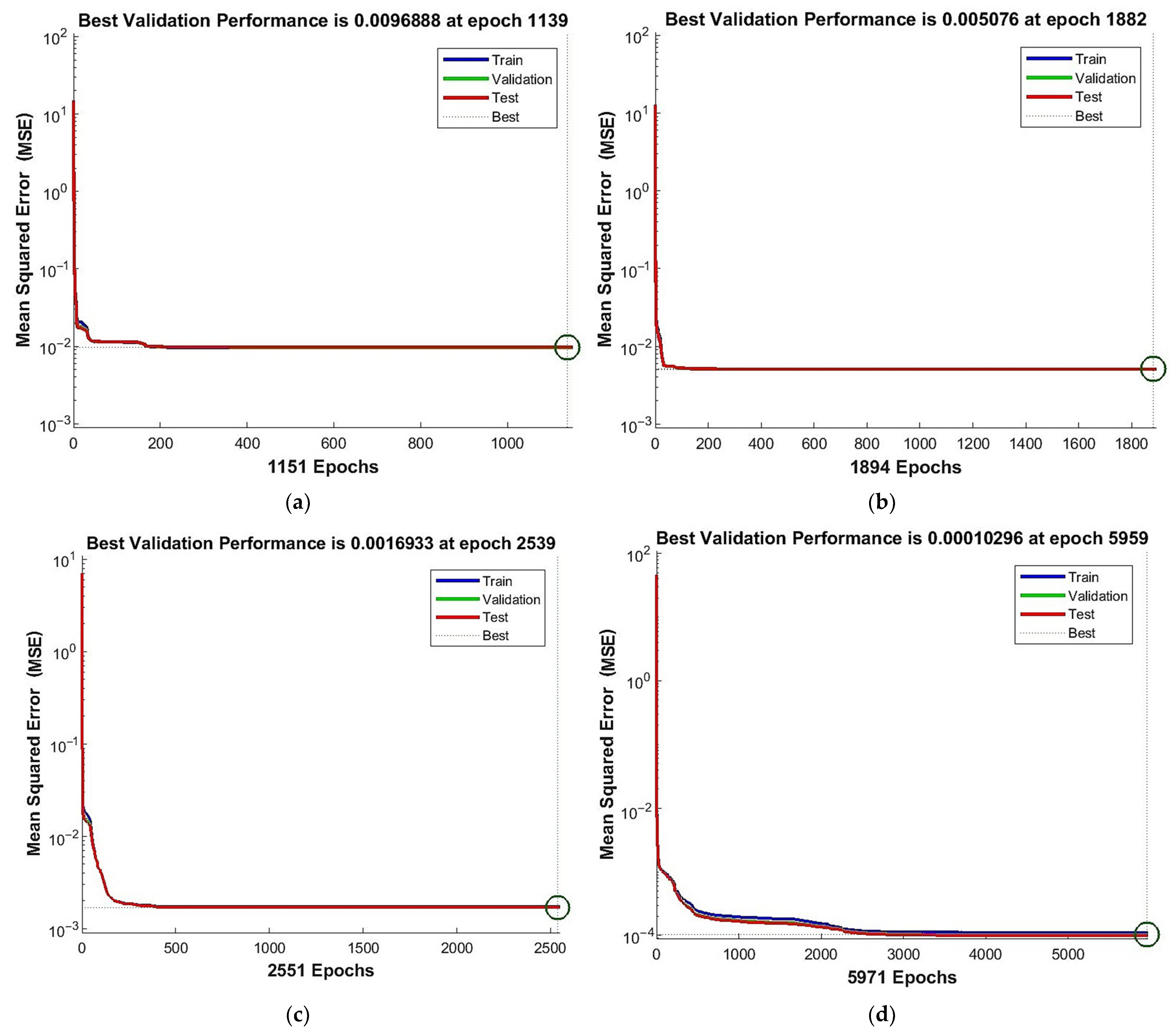
| 0.0096888 | 1.00 | 1139 | 1.00 | |
| 0.005076 | 0.52 | 1882 | 1.65 | |
| 0.0016933 | 0.17 | 2539 | 2.23 | |
| 0.00010296 | 0.01 | 5959 | 5.23 |
Publisher’s Note: MDPI stays neutral with regard to jurisdictional claims in published maps and institutional affiliations. |
© 2022 by the authors. Licensee MDPI, Basel, Switzerland. This article is an open access article distributed under the terms and conditions of the Creative Commons Attribution (CC BY) license (https://creativecommons.org/licenses/by/4.0/).
Share and Cite
Stręk, A.M.; Dudzik, M.; Machniewicz, T. Specifications for Modelling of the Phenomenon of Compression of Closed-Cell Aluminium Foams with Neural Networks. Materials 2022, 15, 1262. https://doi.org/10.3390/ma15031262
Stręk AM, Dudzik M, Machniewicz T. Specifications for Modelling of the Phenomenon of Compression of Closed-Cell Aluminium Foams with Neural Networks. Materials. 2022; 15(3):1262. https://doi.org/10.3390/ma15031262
Chicago/Turabian StyleStręk, Anna M., Marek Dudzik, and Tomasz Machniewicz. 2022. "Specifications for Modelling of the Phenomenon of Compression of Closed-Cell Aluminium Foams with Neural Networks" Materials 15, no. 3: 1262. https://doi.org/10.3390/ma15031262
APA StyleStręk, A. M., Dudzik, M., & Machniewicz, T. (2022). Specifications for Modelling of the Phenomenon of Compression of Closed-Cell Aluminium Foams with Neural Networks. Materials, 15(3), 1262. https://doi.org/10.3390/ma15031262