

Characterization of Inclusion Size Distributions in Steel Wire Rods

 and
and
Abstract
1. Introduction
2. Background
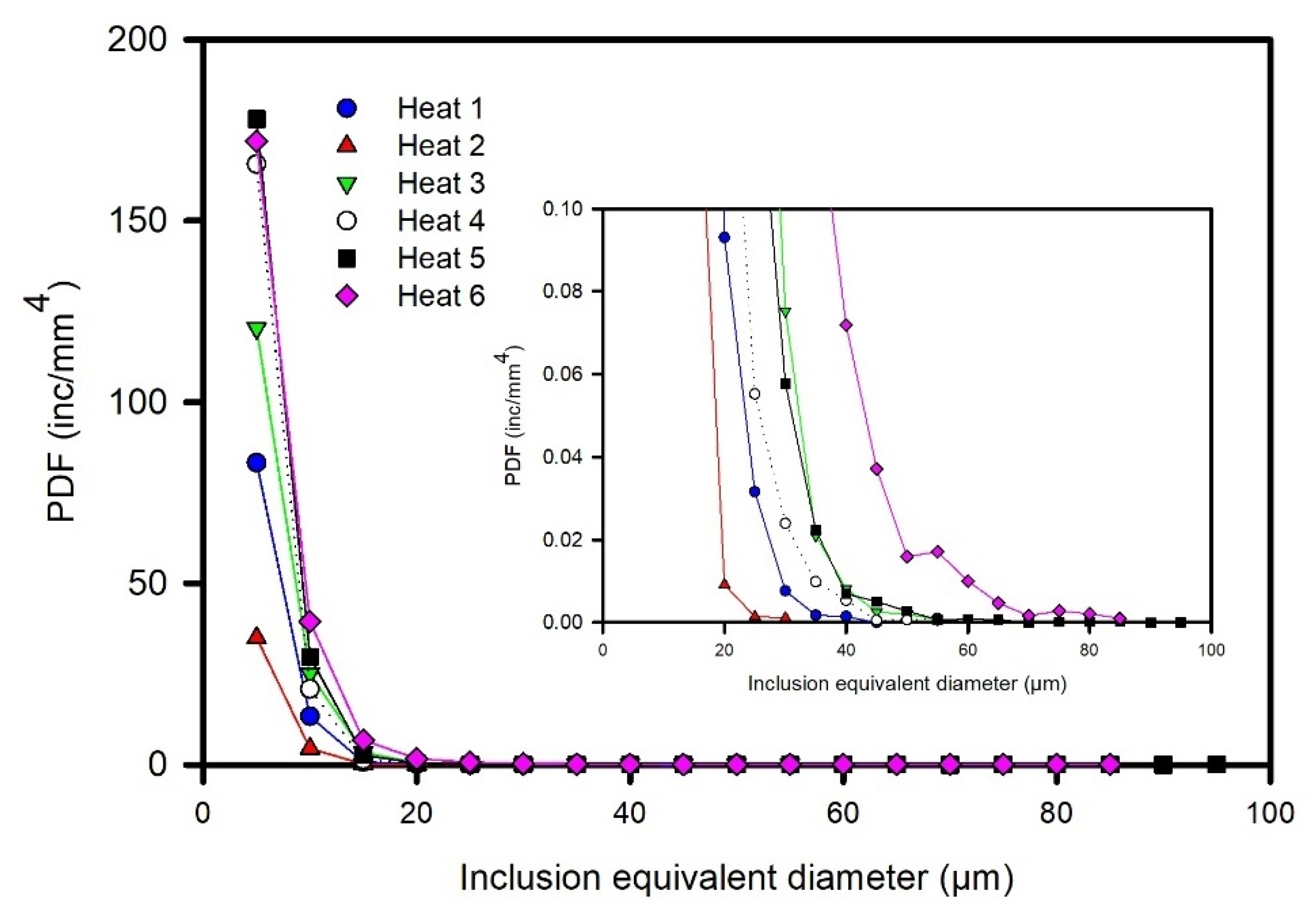
2.1. PDF Approach
2.2. ASTM E2283 Standard
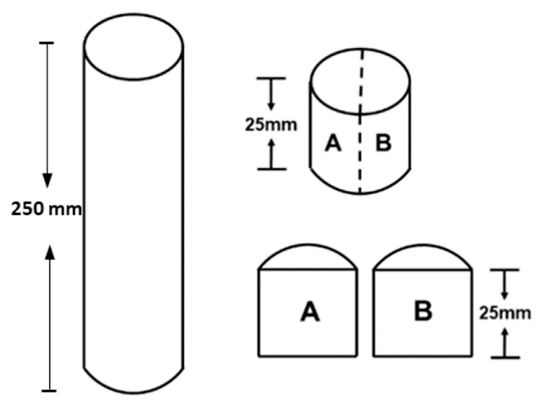
3. Materials and Methods
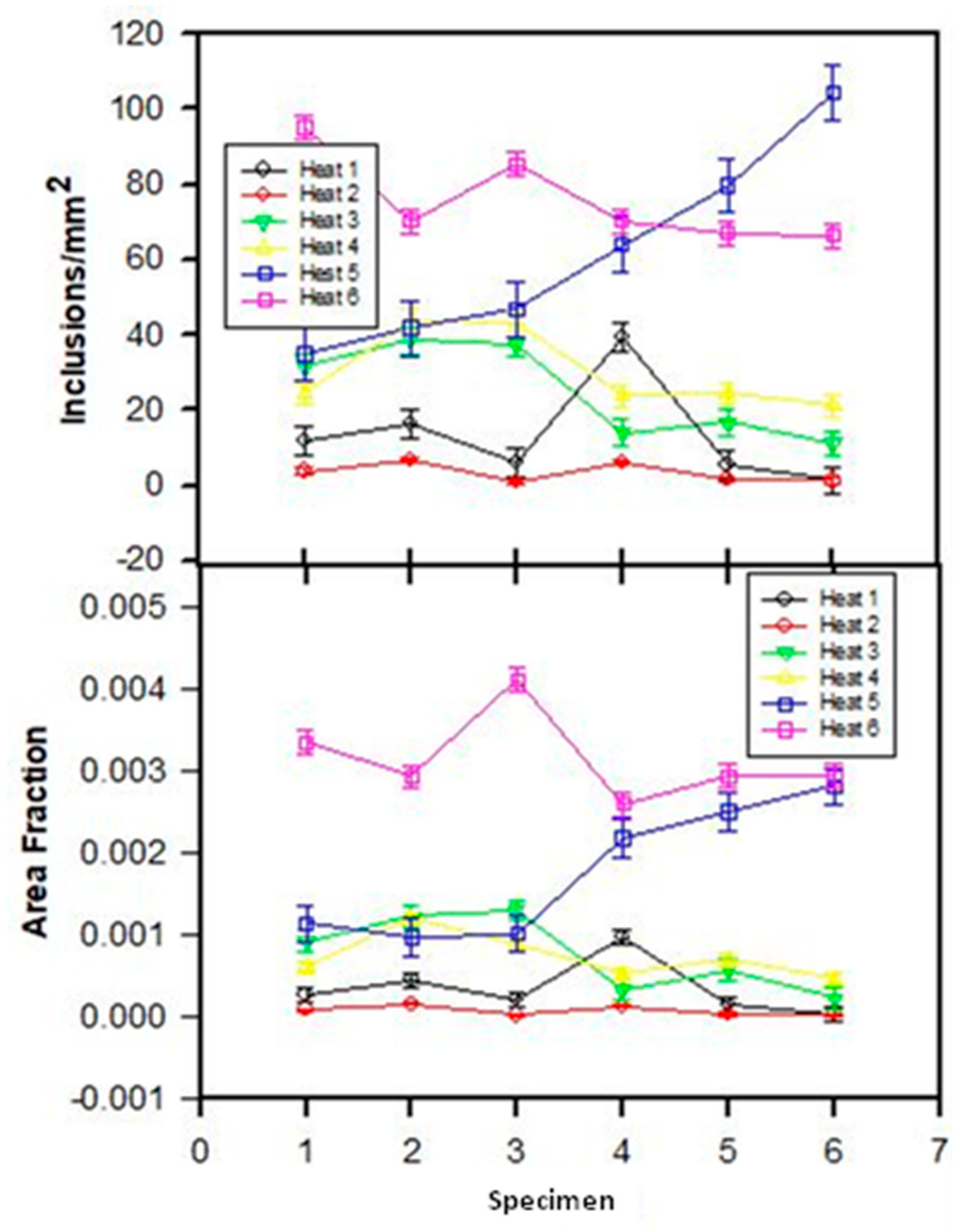
4. Results and Discussion
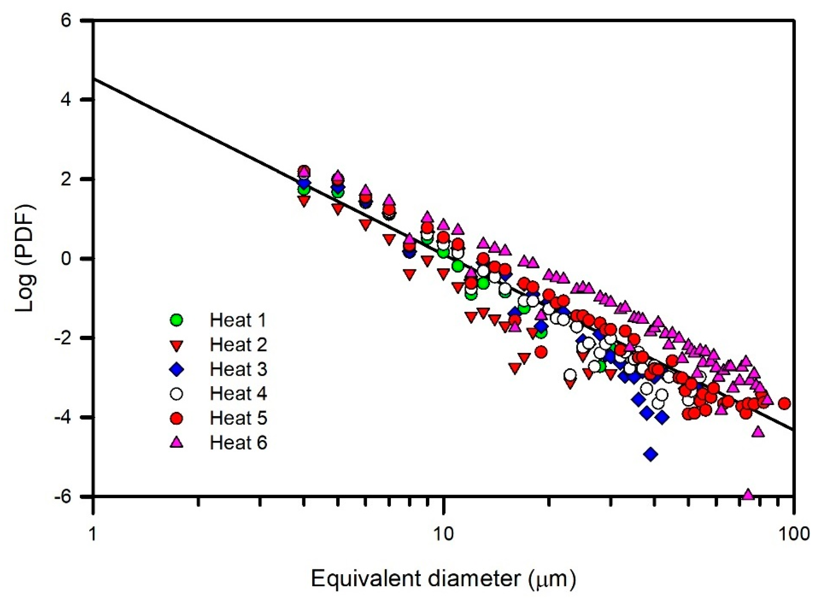
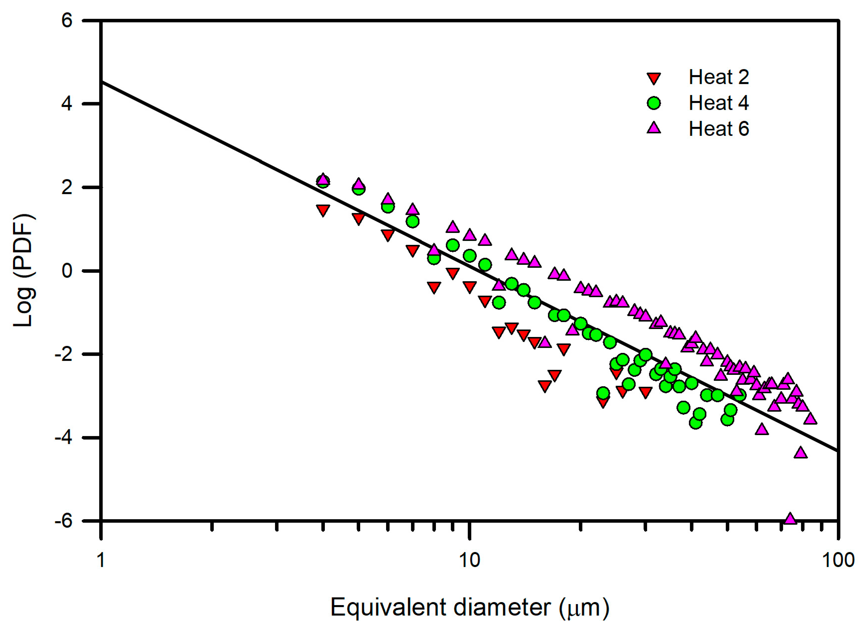
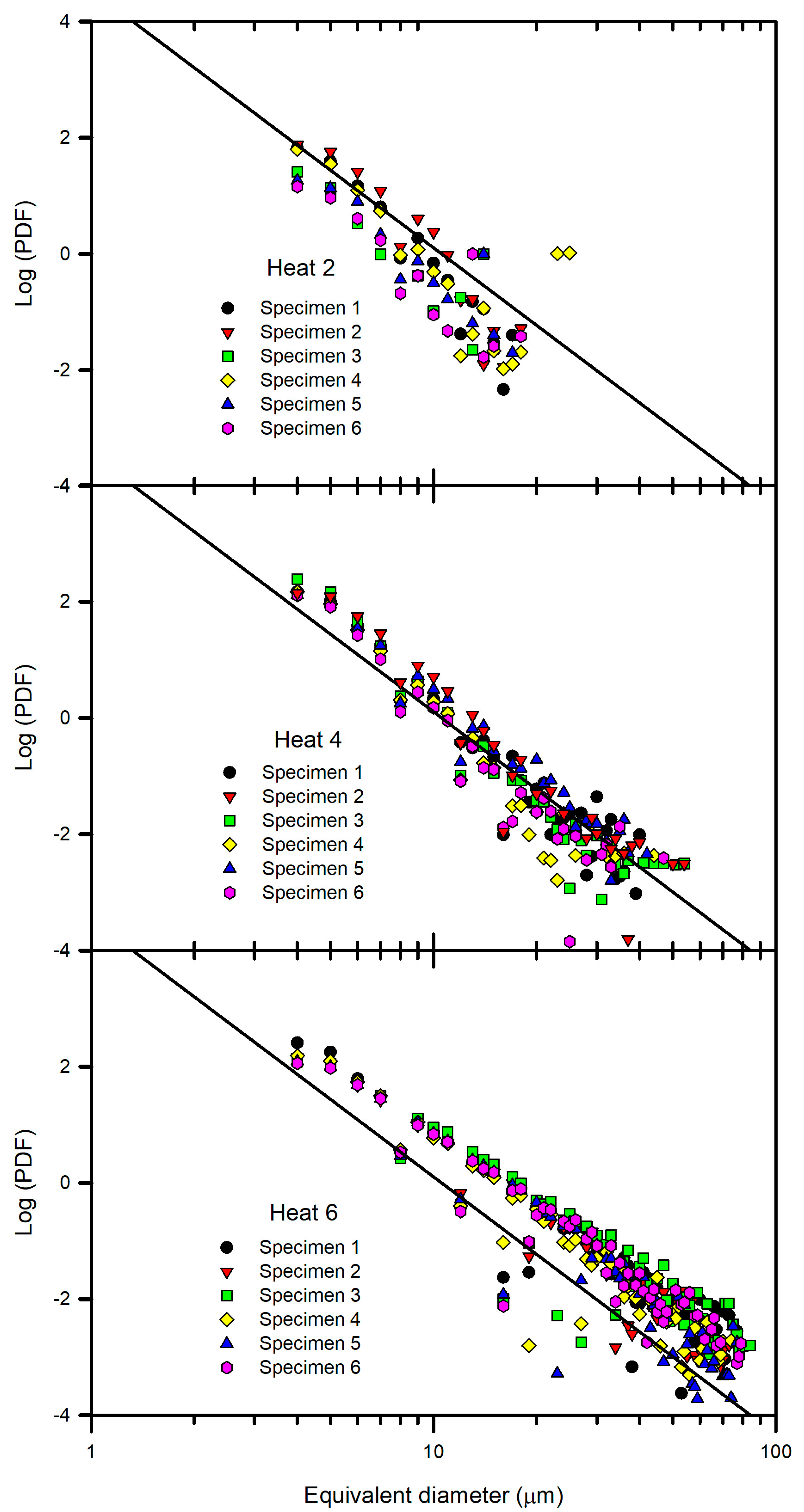
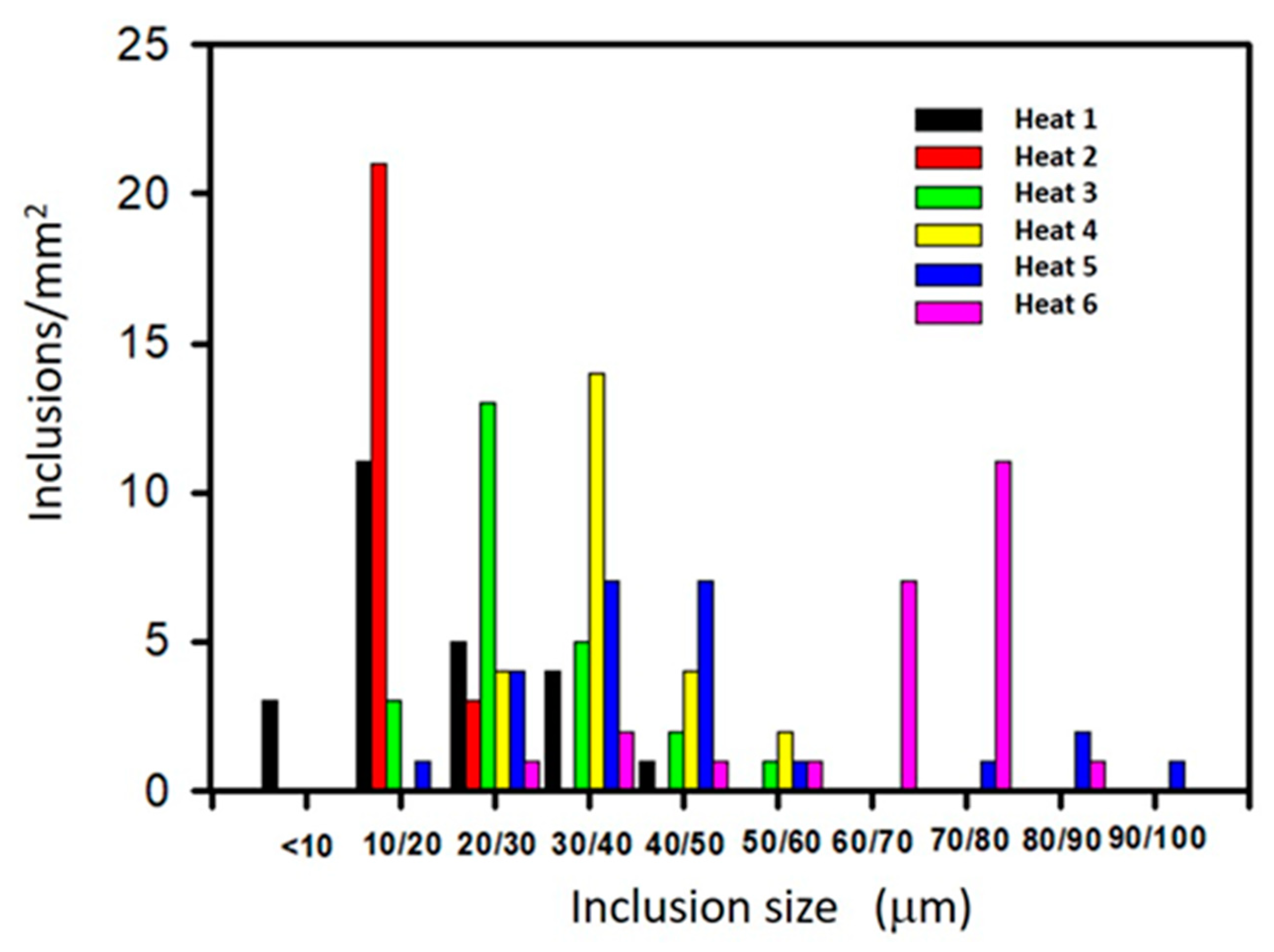
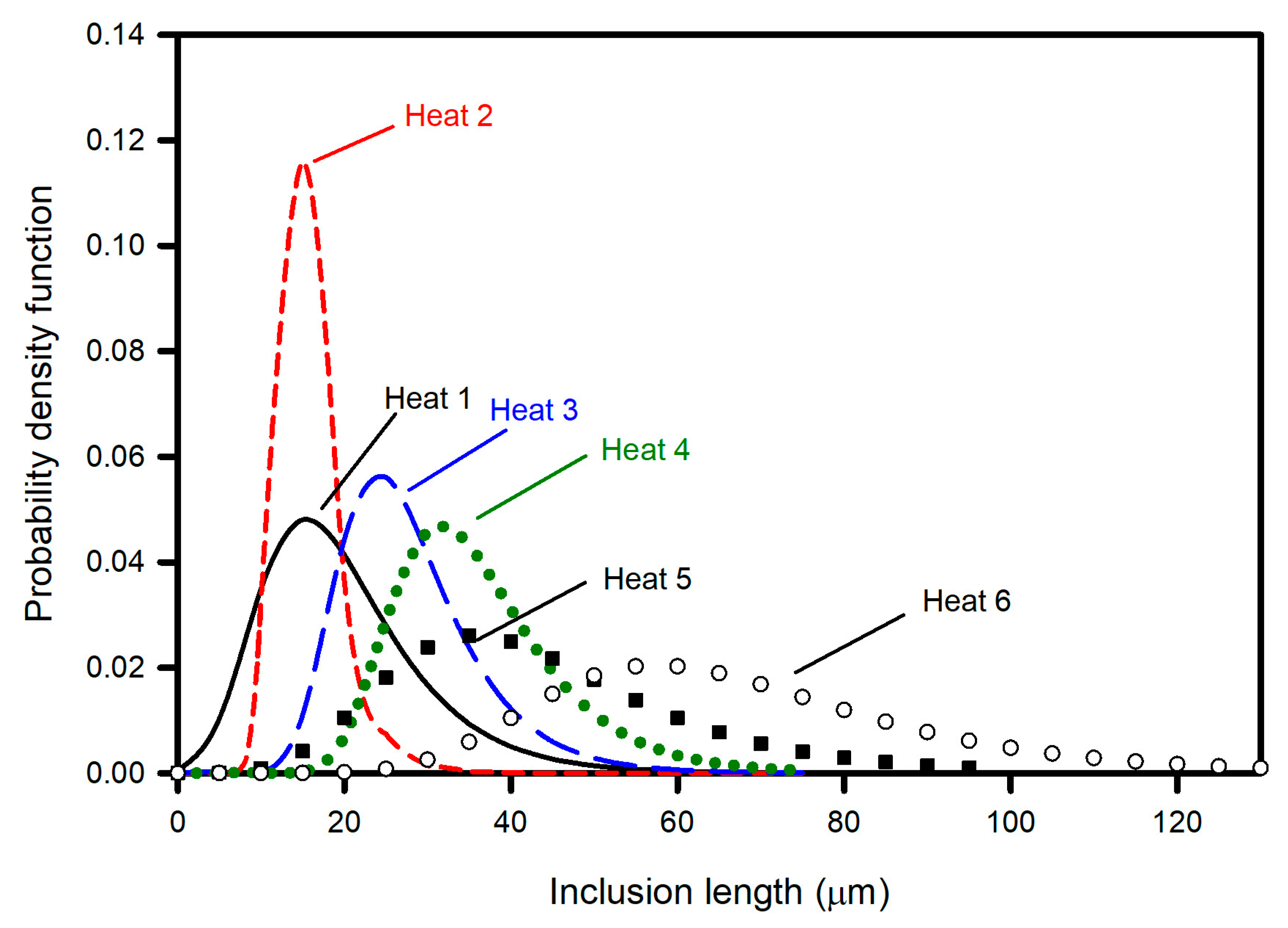
4.1. Population Density Function PDF
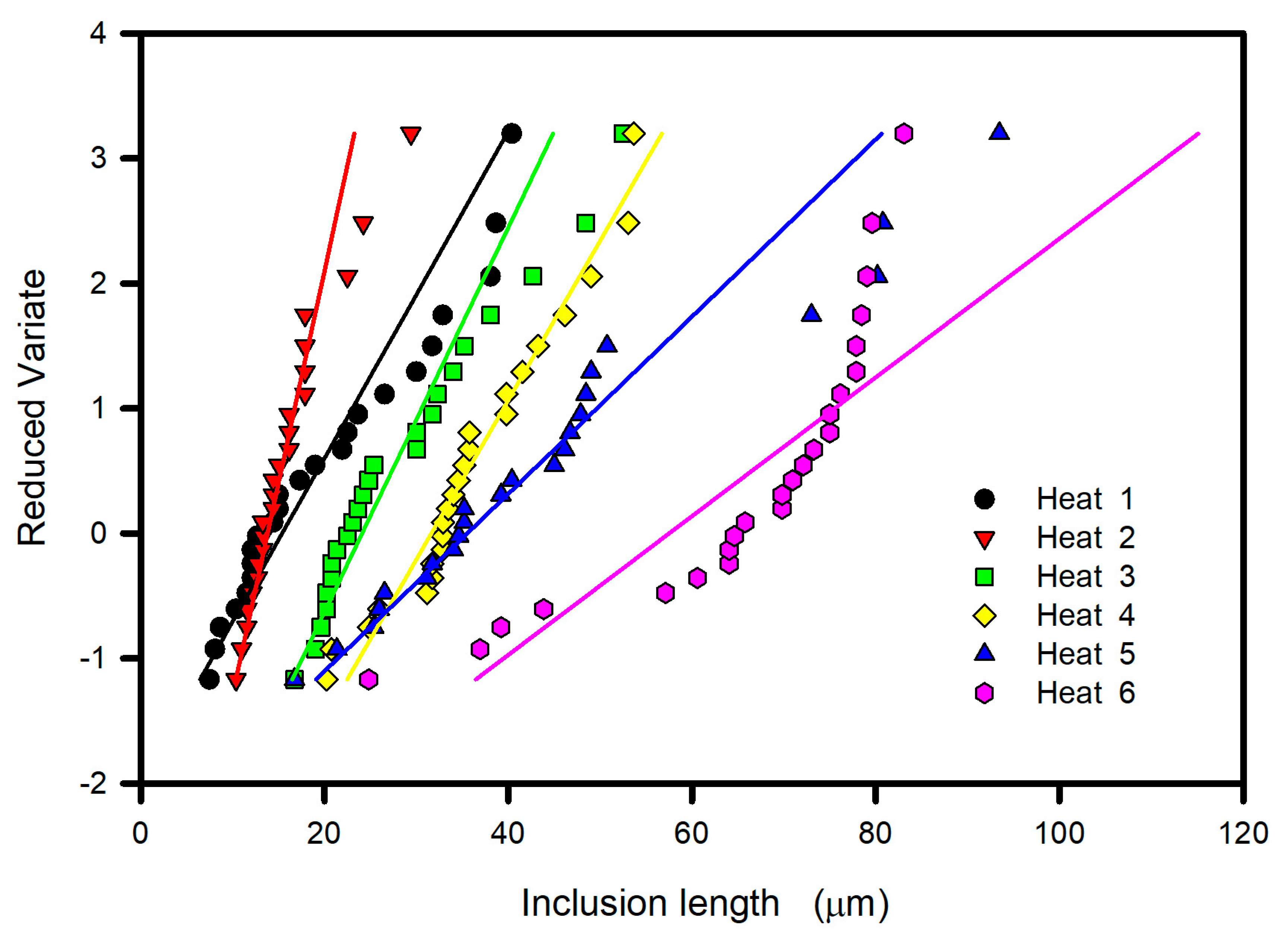
4.2. Extreme Value Distribution Analysis
5. Conclusions
- Heats were listed in decreasing order of inclusion cleanliness based on the analysis of the linear logarithmic representation of PDFs.
- No new inclusions were formed after the ladle treatment process, as inferred from the linear behavior of the logarithmic representation of PDFs, a power-law-type with time. Hence, the evolution of inclusion distribution was associated with growth, breakage, and the removal of inclusions.
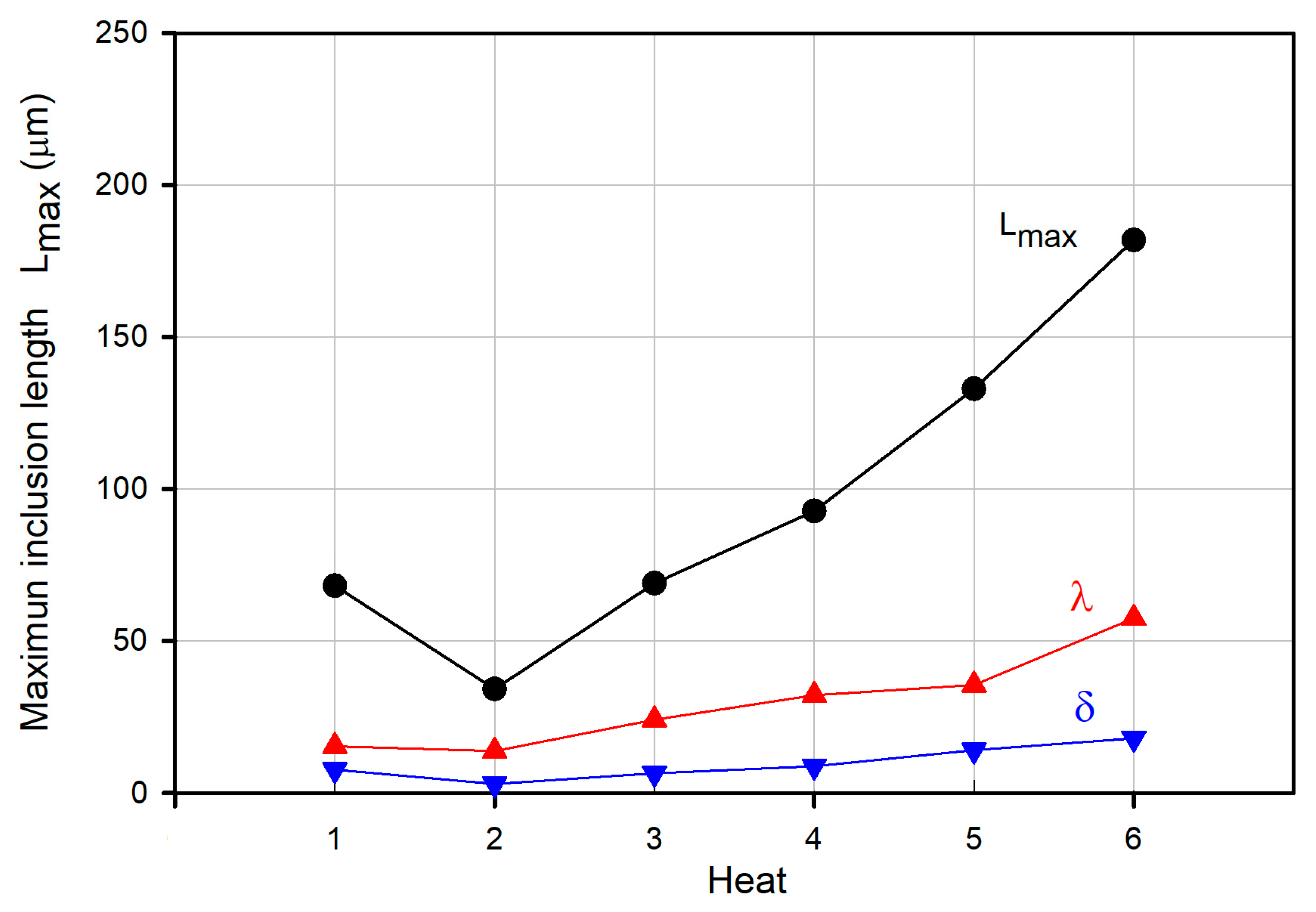
- Heats were listed in decreasing order of inclusion cleanliness using the maximum inclusion length parameter Lmax. The use of the extreme value statistics procedure specified in the ASTM E2283 standard led to a statistical comparison of Lmax.
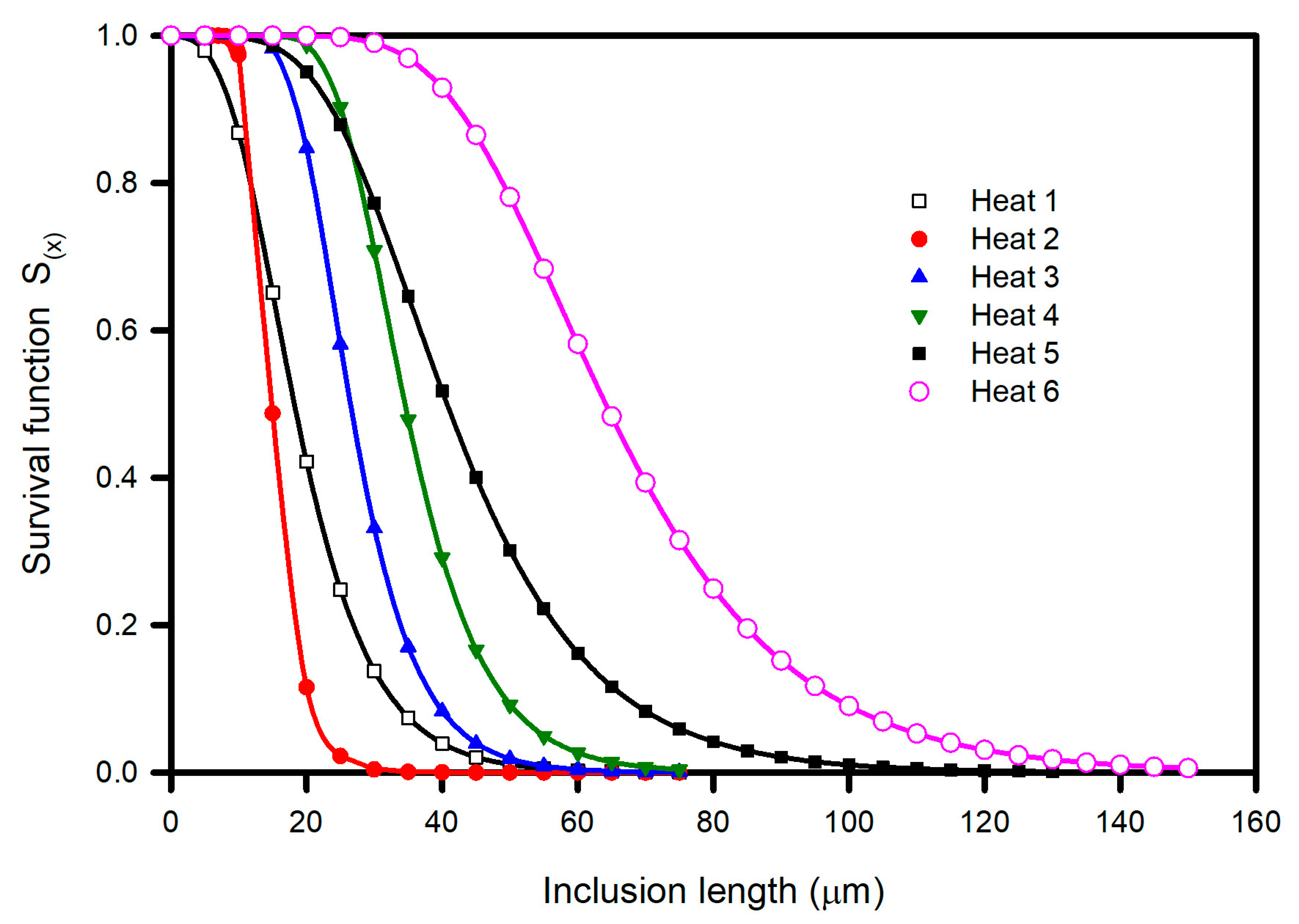
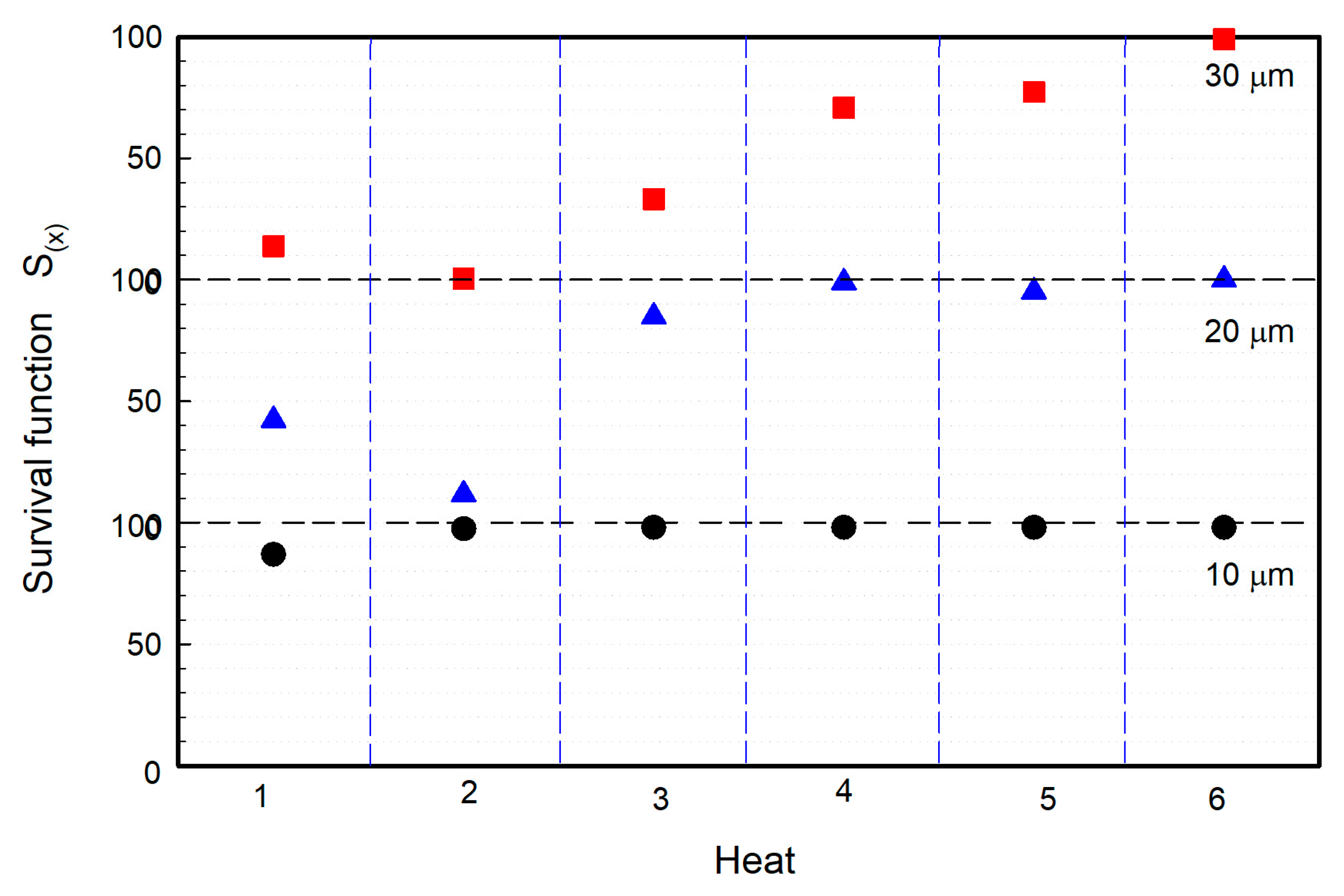
- Heats were ordered by considering the survival function S(x) values (probability of finding an inclusion larger than a “critical” inclusion length) estimated using the GEV theory. It was shown that the order can change depending on the critical value.
Author Contributions
Funding
Acknowledgments
Conflicts of Interest
References
- Kaushik, P.; Lehmann, J.; Nadif, M. State of the Art in Control of Inclusions, Their Characterization, and Future Requirements. Met. Mater. Trans. A 2012, 43, 710–725. [Google Scholar] [CrossRef]
- Pretorius, E.B.; Oltmann, H.G.; Schart, B.T. An Overview of Steel Cleanliness from an Industry Perspective. In AISTech Proceedings 2013; Association for Iron and Steel Technology: Warrendale, PA, USA, 2013; pp. 6–9. [Google Scholar]
- Higgins, M. Measurement of crystal size distributions. Am. Miner. 2000, 85, 1105–1116. [Google Scholar] [CrossRef]
- Atkinson, H.V.; Shi, G. Characterization of Inclusions in Clean Steels: A Review Including the Statistics of Extremes Methods. Prog. Mater. Sci. 2003, 48, 457–520. [Google Scholar] [CrossRef]
- Van Ende, M.-A.; Guo, M.; Zinngrebe, E.; Blanpain, B.; Jung, I.-H. Evolution of Non-Metallic Inclusions in Secondary Steelmaking: Learning from Inclusion Size Distributions. ISIJ Int. 2013, 53, 1974–1982. [Google Scholar] [CrossRef]
- Zinngrebe, E.; Van Hoek, C.; Visser, H.; Westendorp, A.; Jung, I.H. Inclusion Population Evolution in Ti-alloyed Al-killed Steel during Secondary Steelmaking Process. ISIJ Int. 2012, 52, 52–61. [Google Scholar] [CrossRef]
- Bindeman, I.N. Fragmentation Phenomena in Populations of Magmatic Crystals. Am. Miner. 2005, 90, 1801–1815. [Google Scholar] [CrossRef]
- Piva, S.; Pistorius, P. Ferrosilicon-Based Calcium Treatment of Aluminum-Killed and Silicomanganese-Killed Steels. Metall. Mater. Trans. B 2021, 52, 6–14. [Google Scholar] [CrossRef]
- Shu, Q.; Alatarvas, T.; Visuri, V.-V.; Fabritus, T. Modelling the Nucleation, Growth and Agglomeration of Alumina Inclusion in Molten Steel by Combining Kampmann-Wagner Numerical Model with Particle Size Grouping Method. Metall. Mater. Trans. B 2021, 52, 1818–1829. [Google Scholar] [CrossRef]
- Murakami, Y. Inclusion Rating by Statistics of Extreme Values and Its Application to Fatigue Strength Prediction and Quality Control of Materials. Int. J. Fatigue 1996, 3, 215. [Google Scholar] [CrossRef]
- ASTM E2283-08; Extreme Value Analysis of Nonmetallic Inclusions in Steel and Other Microstructural Features. ASTM International: West Conshohocken, PA, USA, 2014.
- Kumar, P.V.; Balachandran, G. Microinclusion Evaluation Using Various Standards. Trans. Indian Inst. Met. 2019, 72, 877–888. [Google Scholar] [CrossRef]
- Fuchs, D.; Tobie TStahl, K. Challenges in Determination of Microscopic Degree of Cleanliness in Ultra-Clean Gear Steels. J. Iron Steel Res. Int. 2022, 29, 1583–1600. [Google Scholar] [CrossRef]
- Meng, Y.; Li, J.; Wang, K.; Zhu, H. Effect of the Bloom-Heating Process on the Inclusion Size of Si-Killed Spring Steel Wire Rod. Metall. Mater. Trans. B 2022, 53, 2647–2656. [Google Scholar] [CrossRef]
- Tian, L.; Liu, L.; Ma, B.; Zaïri, F.; Ding, N.; Guo, W.; Xu, N.; Xu, H.; Zhang, M. Evaluation of Maximum Non-Metallic Inclusion Sizes in steel by Statistics of Extreme Values Method Based on Micro-CT Imaging. Metall. Res. Technol. 2022, 119, 202. [Google Scholar] [CrossRef]
- Gulbin, Y. On Estimation and Hypothesis Testing of the Grain Size Distribution by the Saltykov Method. Image Anal. Stereol. 2008, 27, 163–174. [Google Scholar] [CrossRef]
- Takahashi, J.; Suito, H. Evaluation of the Accuracy of the Three-Dimensional Size Distribution Estimated from the Schwartz-Saltykov Method. Metall. Mater. Trans. A 2003, 34, 171–181. [Google Scholar] [CrossRef]
- García-Carbajal, A.; Herrera-Trejo, M.; Castro-Cedeño, E.; Castro-Román, M.; Martínez- Enríquez, A. Characterization of Inclusion Populations in Mn-Si Deoxidized Steel. Metall. Mater. Trans. B 2017, 48, 3364–3373. [Google Scholar] [CrossRef]


| Heat | Specimen | Content (wt. %) | |||||
|---|---|---|---|---|---|---|---|
| C | Mn | Si | Cr | P | S | ||
| 1 | 1 | 0.57 | 0.70 | 1.45 | 0.66 | 0.008 | 0.014 |
| 2 | 0.58 | 0.70 | 1.44 | 0.67 | 0.007 | 0.012 | |
| 2 | 1 | 0.54 | 0.68 | 1.43 | 0.65 | 0.008 | 0.014 |
| 2 | 0.57 | 0.70 | 1.45 | 0.66 | 0.007 | 0.014 | |
| 3 | 1 | 0.64 | 0.71 | 1.51 | 0.71 | 0.009 | 0.019 |
| 2 | 0.65 | 0.72 | 1.52 | 0.71 | 0.009 | 0.019 | |
| 4 | 1 | 0.59 | 0.70 | 1.5 | 0.70 | 0.008 | 0.019 |
| 2 | 0.60 | 0.71 | 1.48 | 0.69 | 0.008 | 0.019 | |
| 5 | 1 | 0.60 | 0.70 | 1.5 | 0.66 | 0.007 | 0.17 |
| 2 | 0.58 | 0.71 | 1.52 | 0.70 | 0.008 | 0.17 | |
| 6 | 1 | 0.54 | 0.71 | 1.52 | 0.71 | 0.009 | 0.15 |
| 2 | 0.61 | 0.70 | 1.49 | 0.69 | 0.008 | 0.15 | |
| N° Inclusion | Heat | |||||
|---|---|---|---|---|---|---|
| 1 | 2 | 3 | 4 | 5 | 6 | |
| 1 | 7.5 | 10.4 | 16.7 | 20.2 | 16.7 | 24.8 |
| 2 | 8.1 | 11.0 | 19.0 | 20.8 | 21.4 | 36.9 |
| 3 | 8.7 | 11.5 | 19.6 | 24.8 | 25.4 | 39.2 |
| 4 | 10.4 | 11.5 | 20.2 | 26.0 | 26.0 | 43.9 |
| 5 | 11.6 | 12.1 | 20.2 | 31.2 | 26.5 | 57.1 |
| 6 | 12.1 | 12.7 | 20.8 | 31.7 | 31.2 | 60.6 |
| 7 | 12.1 | 12.7 | 20.8 | 31.7 | 31.7 | 64.0 |
| 8 | 12.1 | 13.3 | 21.4 | 32.9 | 34.0 | 64.0 |
| 9 | 12.7 | 13.3 | 22.5 | 32.9 | 34.6 | 64.6 |
| 10 | 14.4 | 13.3 | 23.1 | 32.9 | 35.2 | 65.8 |
| 11 | 15.0 | 14.4 | 23.7 | 33.45 | 35.2 | 69.8 |
| 12 | 15.0 | 14.4 | 24.2 | 34.0 | 39.2 | 69.8 |
| 13 | 17.3 | 14.4 | 24.8 | 34.6 | 40.4 | 71.0 |
| 14 | 19.0 | 15.0 | 25.4 | 35.2 | 45.0 | 72.1 |
| 15 | 21.9 | 16.2 | 30.0 | 35.8 | 46.2 | 73.3 |
| 16 | 22.5 | 16.2 | 30.0 | 35.8 | 46.7 | 75.0 |
| 17 | 23.7 | 16.2 | 31.7 | 39.8 | 47.9 | 75.0 |
| 18 | 26.5 | 17.9 | 32.3 | 39.8 | 48.5 | 76.2 |
| 19 | 30.0 | 17.9 | 34.0 | 41.5 | 49.0 | 77.9 |
| 20 | 31.7 | 17.9 | 35.2 | 43.3 | 50.8 | 77.9 |
| 21 | 32.9 | 17.9 | 38.1 | 46.2 | 73.0 | 78.5 |
| 22 | 38.1 | 22.6 | 42.7 | 49.0 | 80.2 | 79.0 |
| 23 | 38.7 | 24.2 | 48.5 | 53.1 | 80.8 | 79.6 |
| 24 | 40.4 | 29.4 | 52.5 | 53.7 | 93.5 | 83.1 |
| Parameters | Heat | |||||
|---|---|---|---|---|---|---|
| 1 | 2 | 3 | 4 | 5 | 6 | |
| λ | 15.4 | 13.8 | 24.1 | 32.2 | 35.6 | 57.5 |
| δ | 7.6 | 2.9 | 6.5 | 8.8 | 14.1 | 18.0 |
| L average | 20.0 | 15.7 | 28.2 | 35.8 | 44.1 | 65.8 |
| Standard deviation (Sdev) | 10.4 | 4.6 | 9.6 | 11.8 | 19.8 | 15.3 |
| Maximum length (Lmax) | 68.2 | 34.2 | 69.0 | 92.7 | 132.9 | 181.9 |
| Minimum length Y(Lmin) | 6.9 | 6.9 | 6.9 | 6.9 | 6.9 | 6.9 |
| Standard error (S.E.) | 8.9 | 3.5 | 7.7 | 10.4 | 16.7 | 21.3 |
| Heat 2 | Heat 3 | Heat 4 | Heat 5 | Heat 6 | |
|---|---|---|---|---|---|
| Heat 1 | 53.23 | 22.82 | 2.87 | −26.84 | −67.43 |
| 14.79 | −24.40 | −51.96 | −102.63 | −159.96 | |
| Heat 2 | −17.89 | −36.64 | −64.63 | −104.49 | |
| −51.70 | −80.46 | −132.87 | −190.94 | ||
| Heat 3 | 2.10 | −27.18 | −67.56 | ||
| −49.60 | −100.72 | −158.26 | |||
| Heat 4 | −0.87 | −41.71 | |||
| −79.52 | −136.60 | ||||
| Heat 5 | 5.21 | ||||
| −103.14 |
Publisher’s Note: MDPI stays neutral with regard to jurisdictional claims in published maps and institutional affiliations. |
© 2022 by the authors. Licensee MDPI, Basel, Switzerland. This article is an open access article distributed under the terms and conditions of the Creative Commons Attribution (CC BY) license (https://creativecommons.org/licenses/by/4.0/).
Share and Cite
Huazano-Estrada, P.; Herrera-Trejo, M.; Castro-Román, M.d.J.; Ruiz-Mondragón, J. Characterization of Inclusion Size Distributions in Steel Wire Rods. Materials 2022, 15, 7681. https://doi.org/10.3390/ma15217681
Huazano-Estrada P, Herrera-Trejo M, Castro-Román MdJ, Ruiz-Mondragón J. Characterization of Inclusion Size Distributions in Steel Wire Rods. Materials. 2022; 15(21):7681. https://doi.org/10.3390/ma15217681
Chicago/Turabian StyleHuazano-Estrada, Pablo, Martín Herrera-Trejo, Manuel de J. Castro-Román, and Jorge Ruiz-Mondragón. 2022. "Characterization of Inclusion Size Distributions in Steel Wire Rods" Materials 15, no. 21: 7681. https://doi.org/10.3390/ma15217681
APA StyleHuazano-Estrada, P., Herrera-Trejo, M., Castro-Román, M. d. J., & Ruiz-Mondragón, J. (2022). Characterization of Inclusion Size Distributions in Steel Wire Rods. Materials, 15(21), 7681. https://doi.org/10.3390/ma15217681