
Virtual Development of Process Parameters for Bulk Metallic Glass Formation in Laser-Based Powder Bed Fusion


Abstract
:1. Introduction
2. Modelling of Phase Evolution in PBF-LB
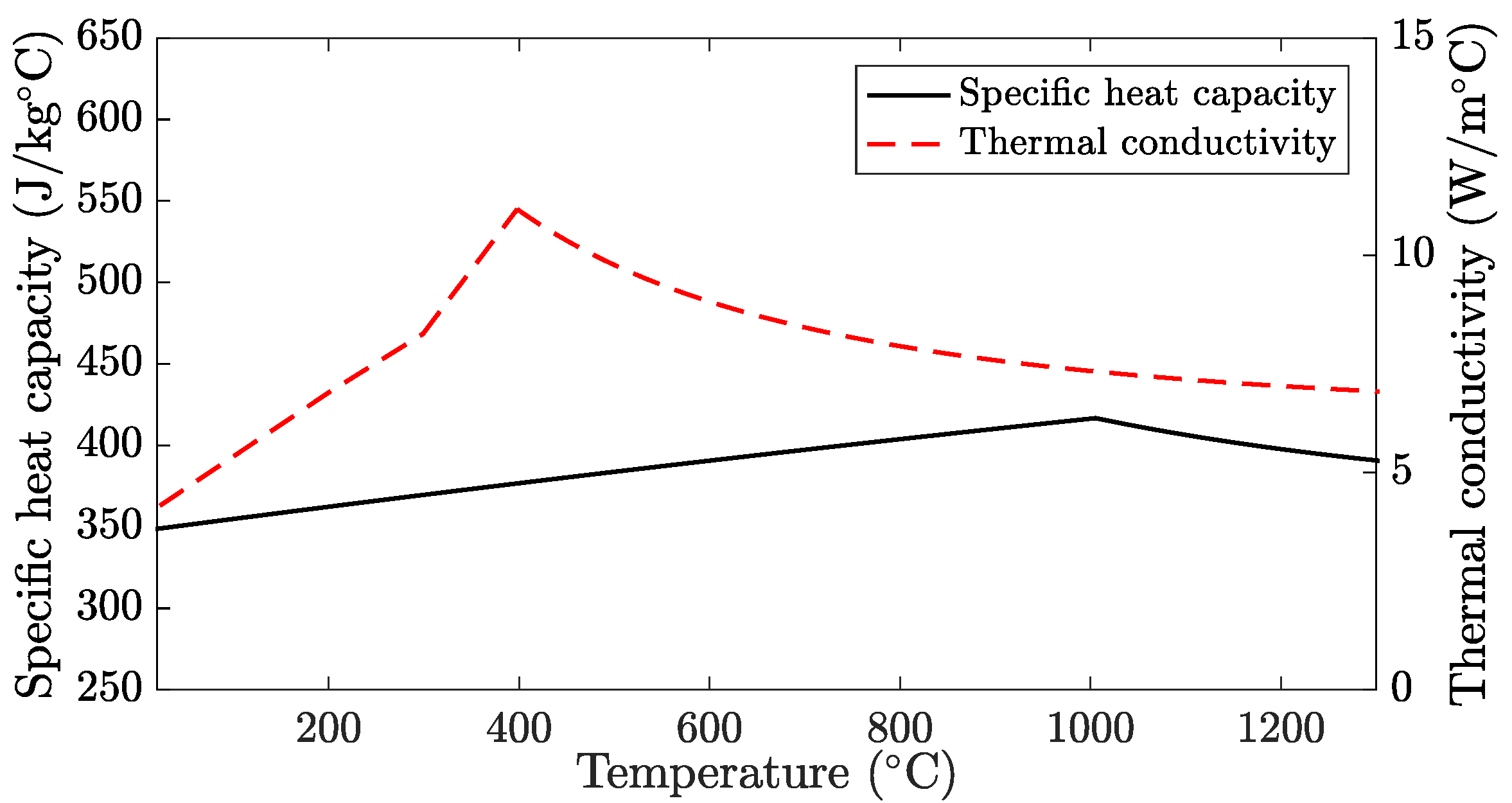
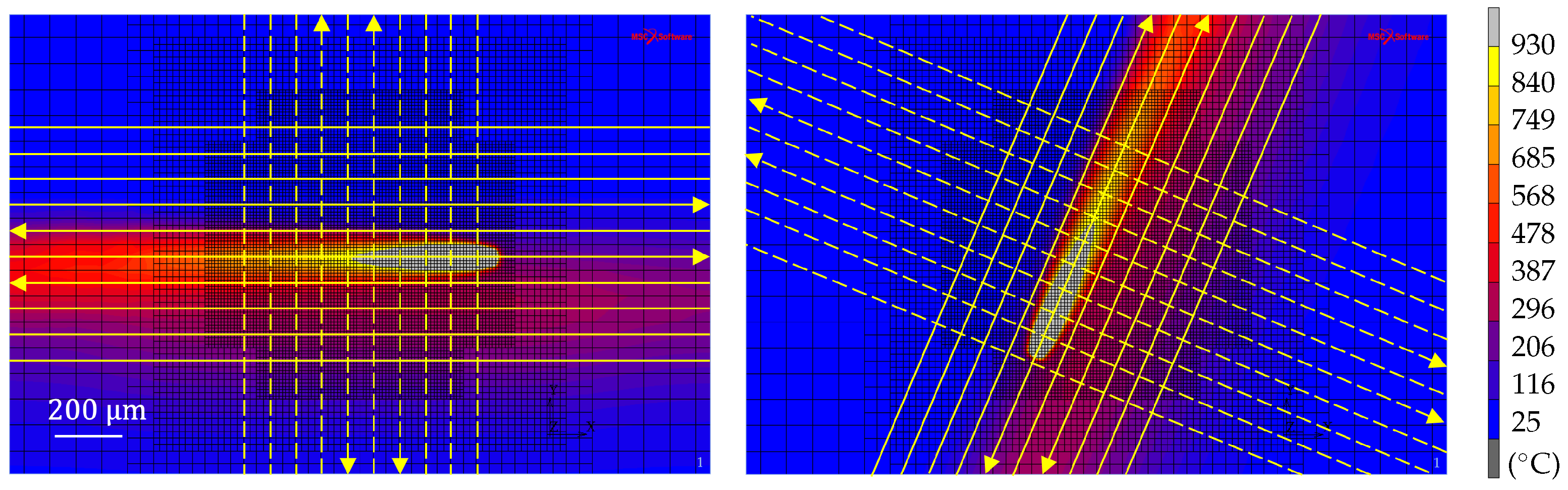
2.1. Thermal Model
2.2. Phase Transformation Model
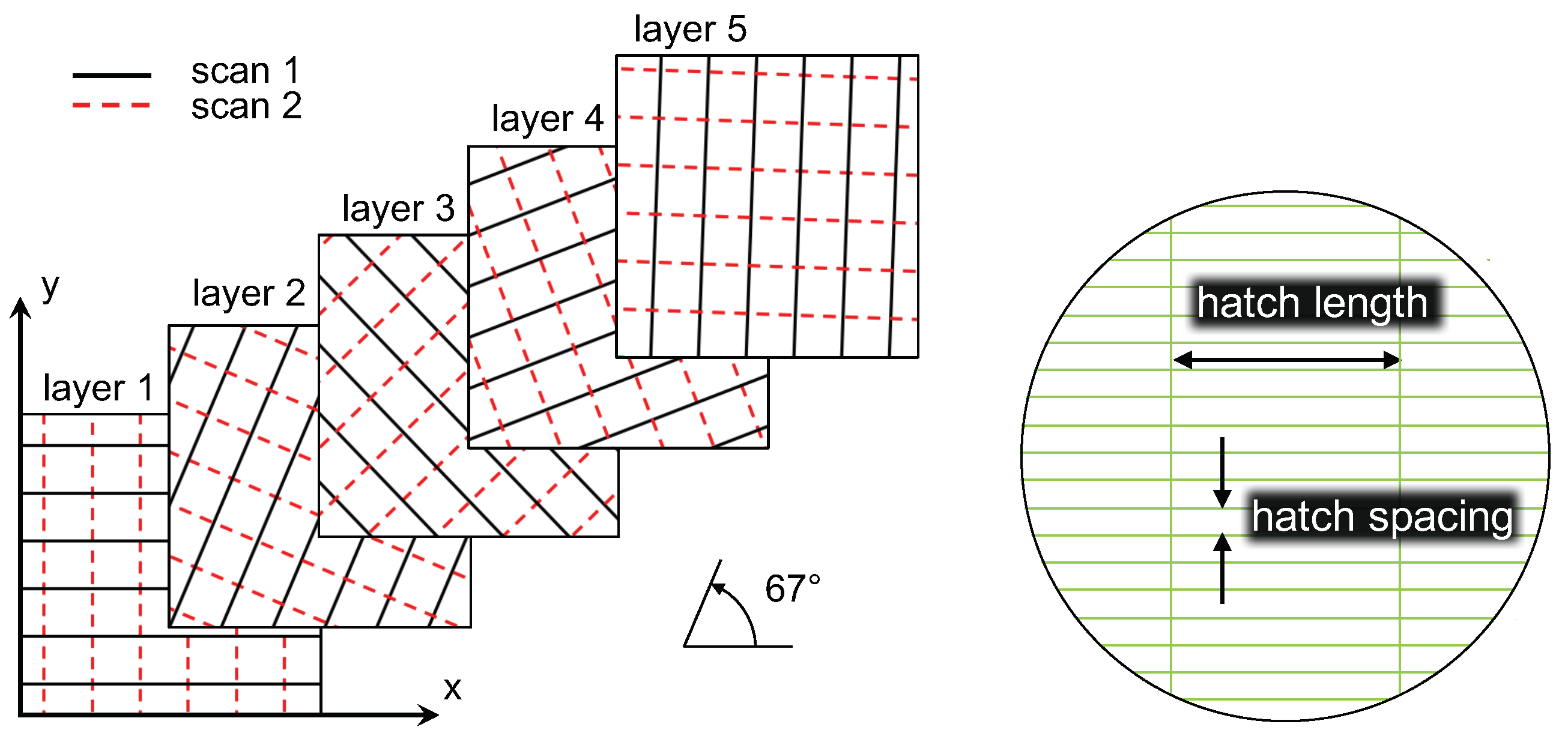
3. Demonstration Methodology
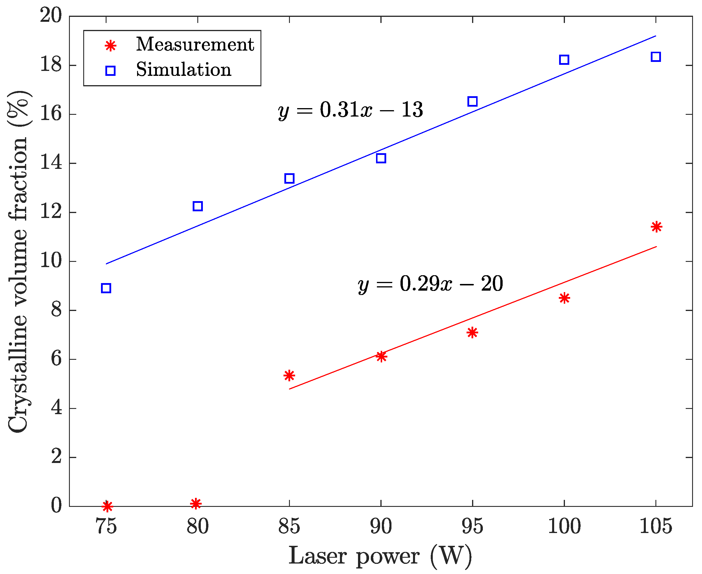
4. Simulation Results
4.1. Laser Power
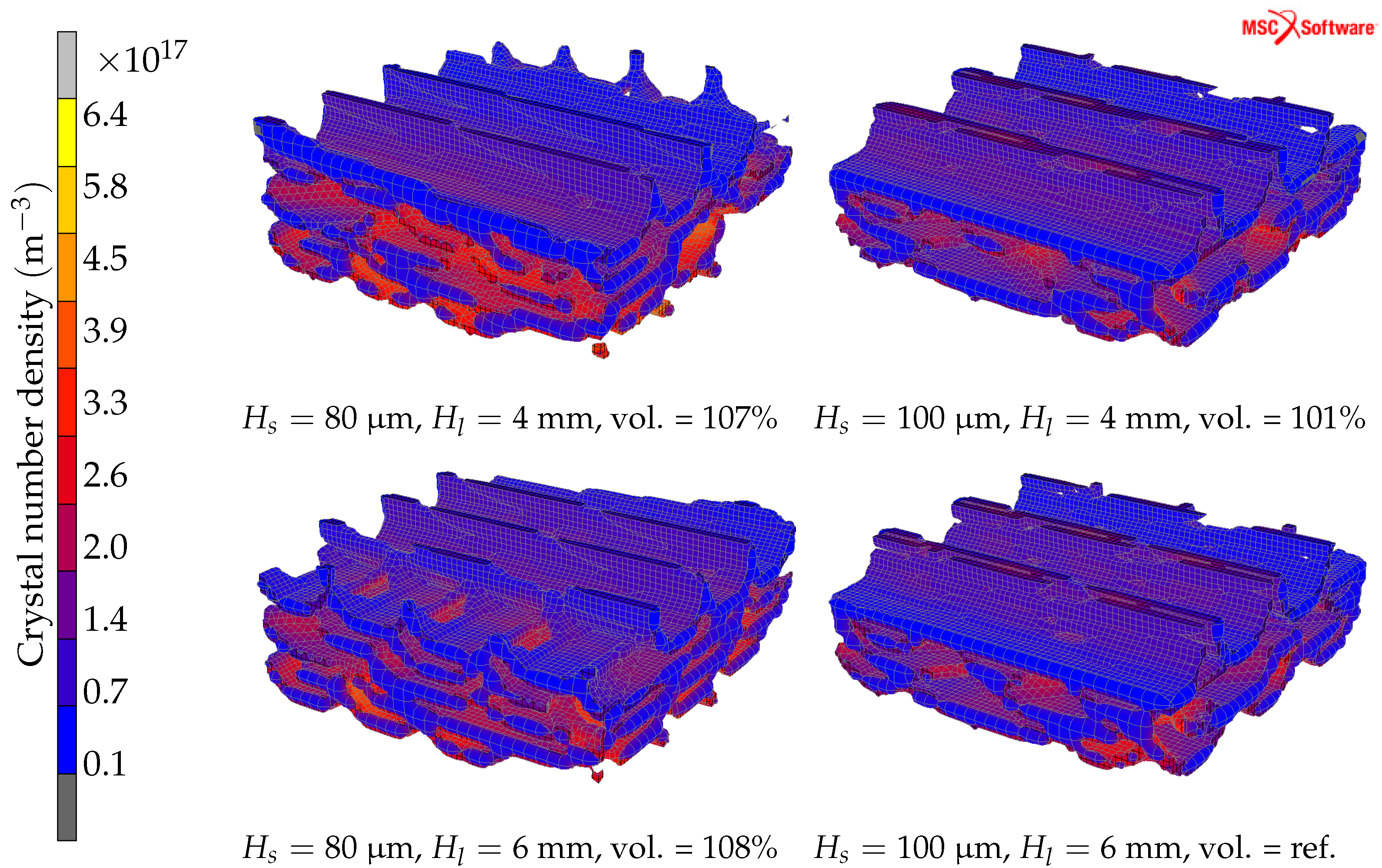
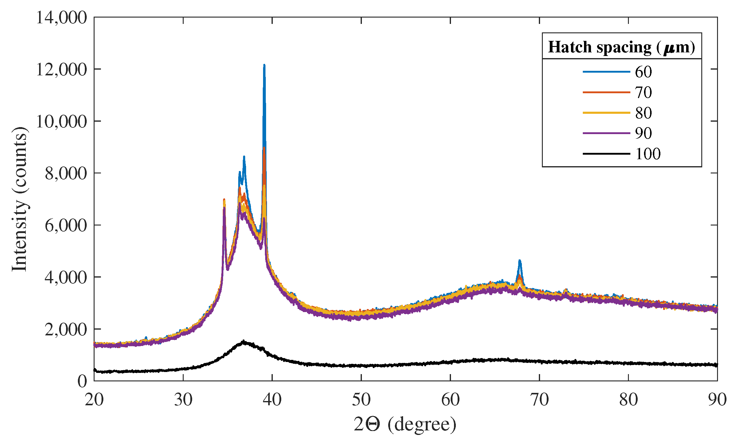
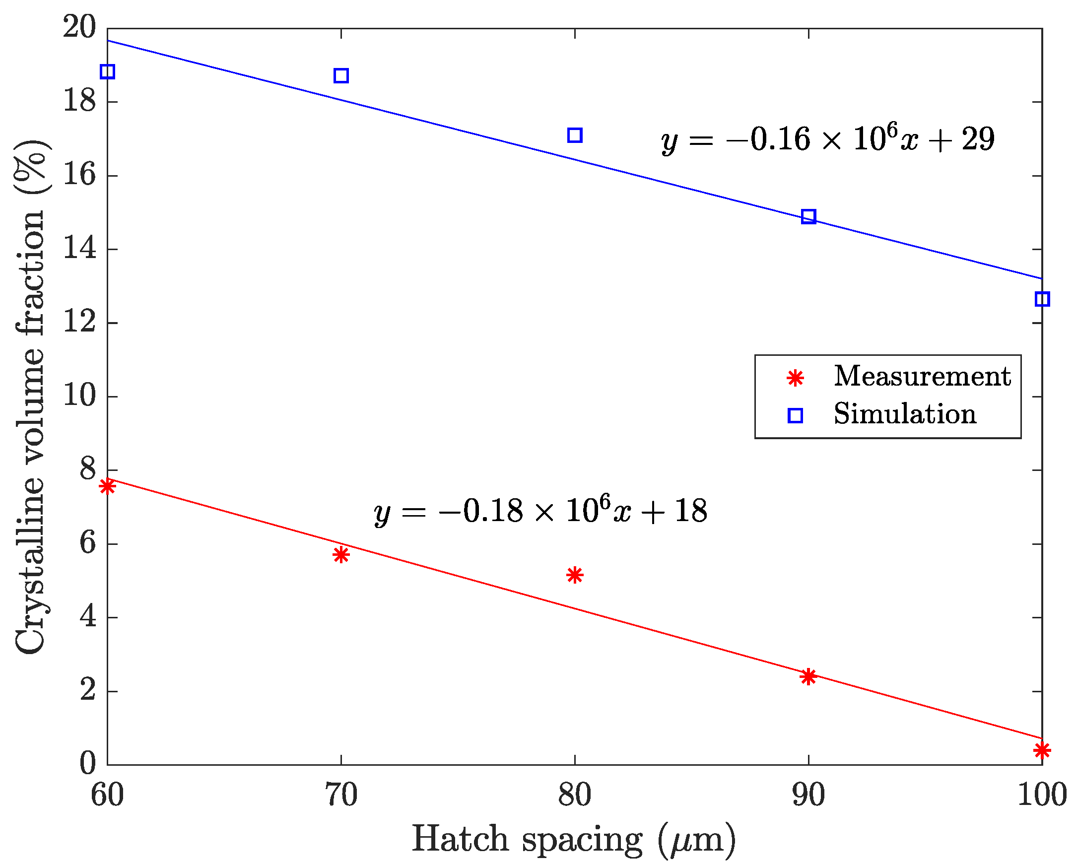
4.2. Hatch Spacing
4.3. Hatch Length and Hatch Spacing
5. Discussion
6. Conclusions
Author Contributions
Funding
Institutional Review Board Statement
Informed Consent Statement
Data Availability Statement
Conflicts of Interest
References
- Miller, M.K.; Liaw, P. Bulk Metallic Glasses: An Overview; Springer: Berlin/Heidelberg, Germany, 2007; p. 290. [Google Scholar]
- Suryanarayana, C.; Inoue, A. Bulk Metallic Glasses; CRC Press: Boca Raton, FL, USA, 2011; p. 565. [Google Scholar]
- Khan, M.M.; Nemati, A.; Rahman, Z.U.; Shah, U.H.; Asgar, H.; Haider, W. Recent Advancements in Bulk Metallic Glasses and Their Applications: A Review. Crit. Rev. Solid State Mater. Sci. 2018, 43, 233–268. [Google Scholar] [CrossRef]
- Schuh, C.A.; Hufnagel, T.C.; Ramamurty, U. Mechanical behavior of amorphous alloys. Acta Mater. 2007, 55, 4067–4109. [Google Scholar] [CrossRef]
- Brechtl, J.; Xie, X.; Wang, Z.; Qiao, J.; Liaw, P.K. Complexity analysis of serrated flows in a bulk metallic glass under constrained and unconstrained conditions. Mater. Sci. Eng. A 2020, 771, 138585. [Google Scholar] [CrossRef]
- Wang, X.D.; Liu, P.; Zhu, Z.W.; Zhang, H.F.; Ren, X.C. High fatigue endurance limit of a Ti-based metallic glass. Intermetallics 2020, 119, 106716. [Google Scholar] [CrossRef]
- Di, S.; Wang, Q.; Zhou, J.; Shen, Y.; Li, J.; Zhu, M.; Yin, K.; Zeng, Q.; Sun, L.; Shen, B. Enhancement of plasticity for FeCoBSiNb bulk metallic glass with superhigh strength through cryogenic thermal cycling. Scr. Mater. 2020, 187, 13–18. [Google Scholar] [CrossRef]
- Bordeenithikasem, P.; Liu, J.; Kube, S.A.; Li, Y.; Ma, T.; Scanley, B.E.; Broadbridge, C.C.; Vlassak, J.J.; Singer, J.P.; Schroers, J. Determination of critical cooling rates in metallic glass forming alloy libraries through laser spike annealing. Sci. Rep. 2017, 7, 7155. [Google Scholar] [CrossRef] [Green Version]
- Sohrabi, N.; Schawe, J.E.; Jhabvala, J.; Löffler, J.F.; Logé, R.E. Critical crystallization properties of an industrial-grade Zr-based metallic glass used in additive manufacturing. Scr. Mater. 2021, 199, 113861. [Google Scholar] [CrossRef]
- Pauly, S.; Löber, L.; Petters, R.; Stoica, M.; Scudino, S.; Kühn, U.; Eckert, J. Processing metallic glasses by selective laser melting. Mater. Today 2013, 16, 37–41. [Google Scholar] [CrossRef]
- Williams, E.; Lavery, N. Laser processing of bulk metallic glass: A review. J. Mater. Process. Technol. 2017, 247, 73–91. [Google Scholar] [CrossRef] [Green Version]
- Liu, H.; Jiang, Q.; Huo, J.; Zhang, Y.; Yang, W.; Li, X. Crystallization in additive manufacturing of metallic glasses: A review. Addit. Manuf. 2020, 36, 101568. [Google Scholar] [CrossRef]
- Jung, H.Y.; Choi, S.J.; Prashanth, K.G.; Stoica, M.; Scudino, S.; Yi, S.; Kühn, U.; Kim, D.H.; Kim, K.B.; Eckert, J. Fabrication of Fe-based bulk metallic glass by selective laser melting: A parameter study. Mater. Des. 2015, 86, 703–708. [Google Scholar] [CrossRef]
- Li, X.; Roberts, M.; O’Keeffe, S.; Sercombe, T. Selective laser melting of Zr-based bulk metallic glasses: Processing, microstructure and mechanical properties. Mater. Des. 2016, 112, 217–226. [Google Scholar] [CrossRef]
- Marattukalam, J.J.; Pacheco, V.; Karlsson, D.; Riekehr, L.; Lindwall, J.; Forsberg, F.; Jansson, U.; Sahlberg, M.; Hjörvarsson, B. Development of process parameters for selective laser melting of a Zr-based bulk metallic glass. Addit. Manuf. 2020, 33, 101124. [Google Scholar] [CrossRef]
- Yang, G.; Lin, X.; Liu, F.; Hu, Q.; Ma, L.; Li, J.; Huang, W. Laser solid forming Zr-based bulk metallic glass. Intermetallics 2012, 22, 110–115. [Google Scholar] [CrossRef]
- Lindwall, J.; Pacheco, V.; Sahlberg, M.; Lundbäck, A.; Lindgren, L.E. Thermal simulation and phase modeling of bulk metallic glass in the powder bed fusion process. Addit. Manuf. 2019, 27, 345–352. [Google Scholar] [CrossRef]
- Shen, Y.; Li, Y.; Tsai, H.L. Evolution of crystalline phase during laser processing of Zr-based metallic glass. J. Non-Cryst. Solids 2018, 481, 299–305. [Google Scholar] [CrossRef]
- Ericsson, A.; Pacheco, V.; Sahlberg, M.; Lindwall, J.; Hallberg, H.; Fisk, M. Transient nucleation in selective laser melting of Zr-based bulk metallic glass. Mater. Des. 2020, 195, 108958. [Google Scholar] [CrossRef]
- Lindwall, J.; Ericsson, A.; Marattukalam, J.J.; Hassila, C.J.; Karlsson, D.; Sahlberg, M.; Fisk, M.; Lundbäck, A. Simulation of phase evolution in a Zr-based glass forming alloy during multiple laser remelting. J. Mater. Res. Technol. 2021, 16, 1165–1178. [Google Scholar] [CrossRef]
- Chiumenti, M.; Neiva, E.; Salsi, E.; Cervera, M.; Badia, S.; Moya, J.; Chen, Z.; Lee, C.; Davies, C. Numerical modelling and experimental validation in Selective Laser Melting. Addit. Manuf. 2017, 18, 171–185. [Google Scholar] [CrossRef] [Green Version]
- Lindwall, J.; Malmelöv, A.; Lundbäck, A.; Lindgren, L.E. Efficiency and Accuracy in Thermal Simulation of Powder Bed Fusion of Bulk Metallic Glass. JOM 2018, 70, 1598–1603. [Google Scholar] [CrossRef]
- Goldak, J.; Chakravarti, A.; Bibby, M. A new finite element model for welding heat sources. Metall. Trans. B 1984, 15, 299–305. [Google Scholar] [CrossRef]
- Heinrich, J.; Busch, R.; Nonnenmacher, B. Processing of a bulk metallic glass forming alloy based on industrial grade Zr. Intermetallics 2012, 25, 1–4. [Google Scholar] [CrossRef]
- Yamasaki, M.; Kagao, S.; Kawamura, Y. Thermal diffusivity and conductivity of Zr55Al10Ni5Cu30 bulk metallic glass. Scr. Mater. 2005, 53, 63–67. [Google Scholar] [CrossRef]
- Perez, M.; Dumont, M.; Acevedo-Reyes, D. Implementation of classical nucleation and growth theories for precipitation. Acta Mater. 2008, 56, 2119–2132. [Google Scholar] [CrossRef]
- Kelton, K.F.; Greer, A.L. Nucleation in Condensed Matter: Applications in Materials and Biology, 1st ed.; Pergamon: Oxford, UK, 2010. [Google Scholar] [CrossRef]
- Kelton, K.F.; Greer, A. Transient nucleation effects in glass formation. J. Non-Cryst. Solids 1986, 79, 295–309. [Google Scholar] [CrossRef]
- Kelton, K.F. Numerical model for isothermal and non-isothermal crystallization of liquids and glasses. J. Non-Cryst. Solids 1993, 163, 283–296. [Google Scholar] [CrossRef]
- Kolmogorov, A. On The Statistical Theory of Metal Crystallization. Izv. Akad. Nauk SSSR Ser. Mat. 1937, 3, 355–360. [Google Scholar] [CrossRef]
- Johnson, W.A.; Mehl, R.F. Reaction kinetics in processes of nucleation and growth. Trans. AIME 1939, 135, 416–442. [Google Scholar] [CrossRef]
- Avrami, M. Kinetics of phase change. I General theory. J. Chem. Phys. 1939, 7, 1103–1112. [Google Scholar] [CrossRef]
- Sohrabi, N.; Jhabvala, J.; Kurtuldu, G.; Stoica, M.; Parrilli, A.; Berns, S.; Polatidis, E.; Van Petegem, S.; Hugon, S.; Neels, A.; et al. Characterization, mechanical properties and dimensional accuracy of a Zr-based bulk metallic glass manufactured via laser powder-bed fusion. Mater. Des. 2021, 199, 109400. [Google Scholar] [CrossRef]


| Hatch Spacing | 80 μm | 100 μm | |
|---|---|---|---|
| Hatch Length | |||
| 4 mm | 17.0% | 12.8% | |
| 5 mm | 17.1% | 12.6% | |
| 6 mm | 17.0% | 11.8% | |
| Hatch Spacing | 80 μm | 100 μm | |
|---|---|---|---|
| Hatch Length | |||
| 4 mm | 3.01 | 1.85 | |
| 5 mm | 2.96 | 1.8 | |
| 6 mm | 2.68 | 1.66 | |
| Hatch Spacing | 80 μm | 100 μm | |
|---|---|---|---|
| Hatch Length | |||
| 4 mm | 179 nm | 143 nm | |
| 5 mm | 176 nm | 139 nm | |
| 6 mm | 175 nm | 131 nm | |
Publisher’s Note: MDPI stays neutral with regard to jurisdictional claims in published maps and institutional affiliations. |
© 2022 by the authors. Licensee MDPI, Basel, Switzerland. This article is an open access article distributed under the terms and conditions of the Creative Commons Attribution (CC BY) license (https://creativecommons.org/licenses/by/4.0/).
Share and Cite
Lindwall, J.; Lundbäck, A.; Marattukalam, J.J.; Ericsson, A. Virtual Development of Process Parameters for Bulk Metallic Glass Formation in Laser-Based Powder Bed Fusion. Materials 2022, 15, 450. https://doi.org/10.3390/ma15020450
Lindwall J, Lundbäck A, Marattukalam JJ, Ericsson A. Virtual Development of Process Parameters for Bulk Metallic Glass Formation in Laser-Based Powder Bed Fusion. Materials. 2022; 15(2):450. https://doi.org/10.3390/ma15020450
Chicago/Turabian StyleLindwall, Johan, Andreas Lundbäck, Jithin James Marattukalam, and Anders Ericsson. 2022. "Virtual Development of Process Parameters for Bulk Metallic Glass Formation in Laser-Based Powder Bed Fusion" Materials 15, no. 2: 450. https://doi.org/10.3390/ma15020450
APA StyleLindwall, J., Lundbäck, A., Marattukalam, J. J., & Ericsson, A. (2022). Virtual Development of Process Parameters for Bulk Metallic Glass Formation in Laser-Based Powder Bed Fusion. Materials, 15(2), 450. https://doi.org/10.3390/ma15020450