
Innovative Design Methodology for Patient-Specific Short Femoral Stems


Abstract
1. Introduction
2. Materials and Methods
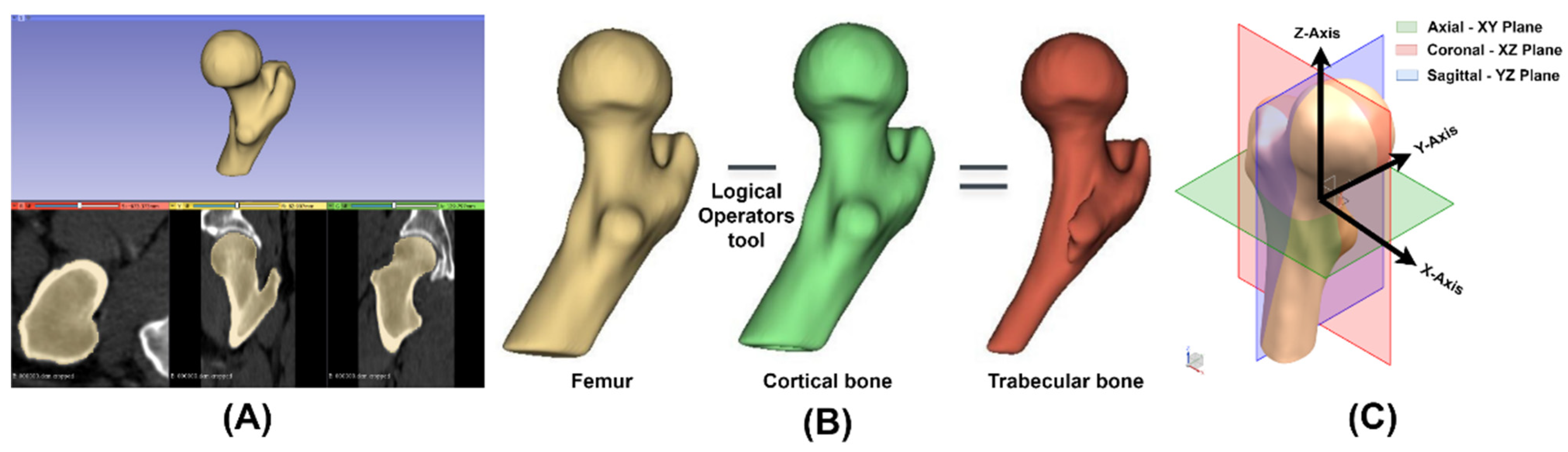
2.1. Virtual Model
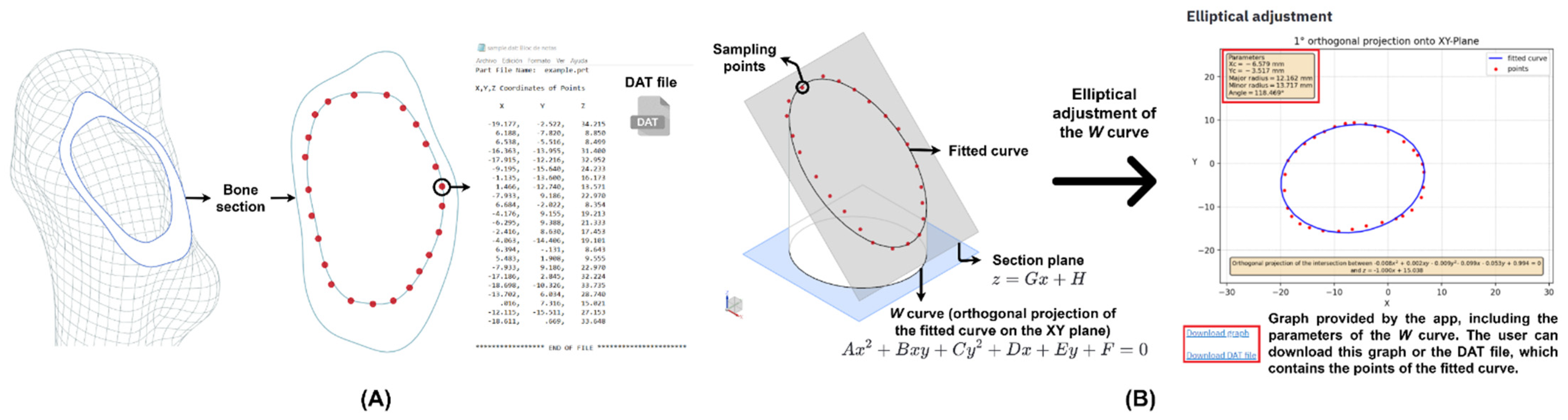
2.2. Elliptical Adjustment App
2.3. Morphological Study
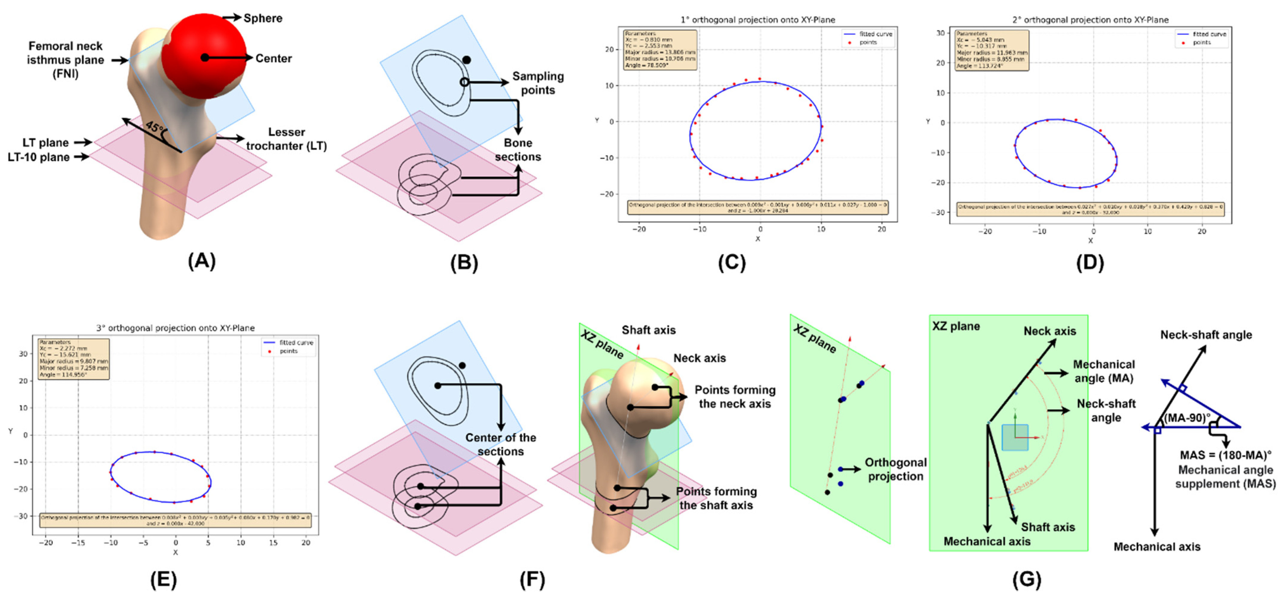
2.3.1. Neck–Shaft and Mechanical Angle
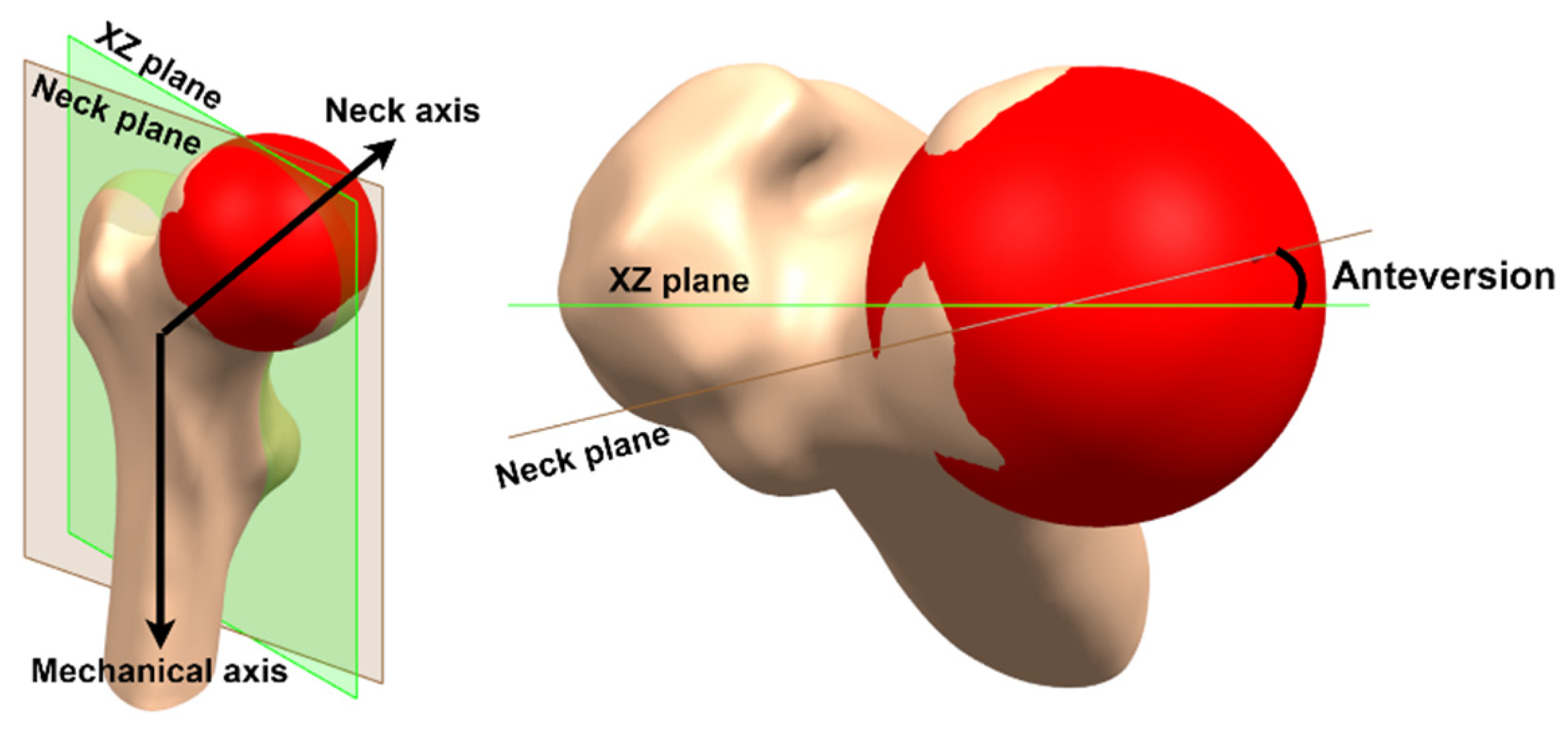
2.3.2. Anteversion
2.3.3. Offset
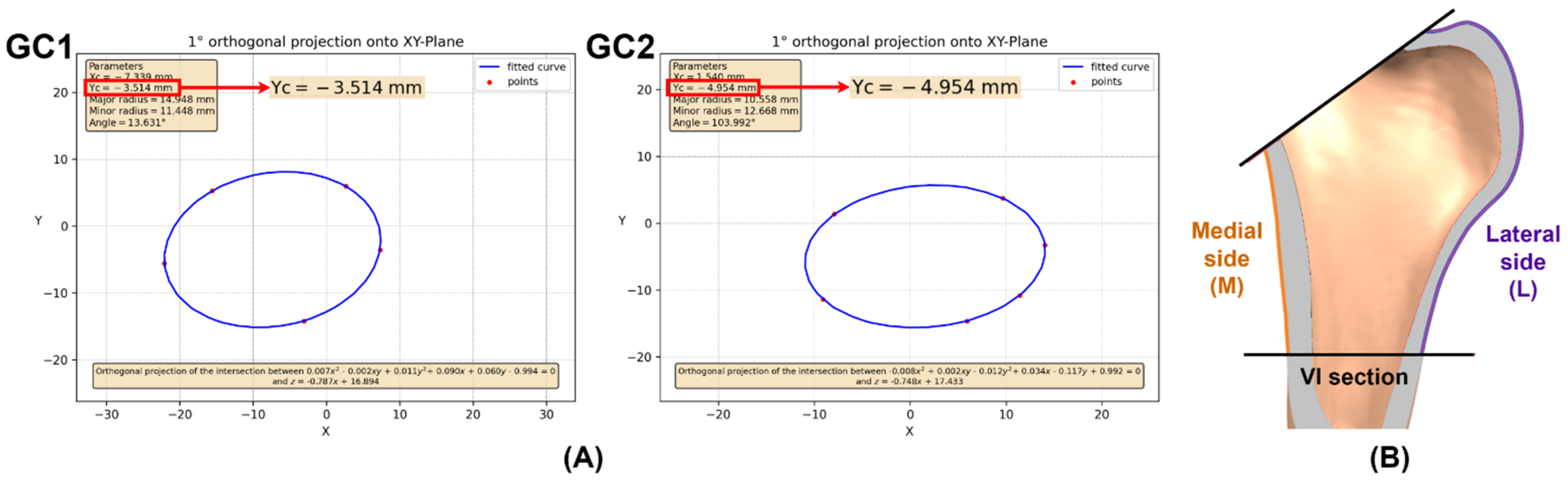
2.3.4. Femoral Cavity
2.4. Custom Design
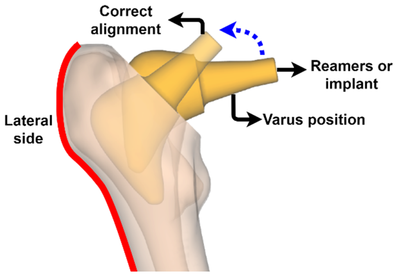
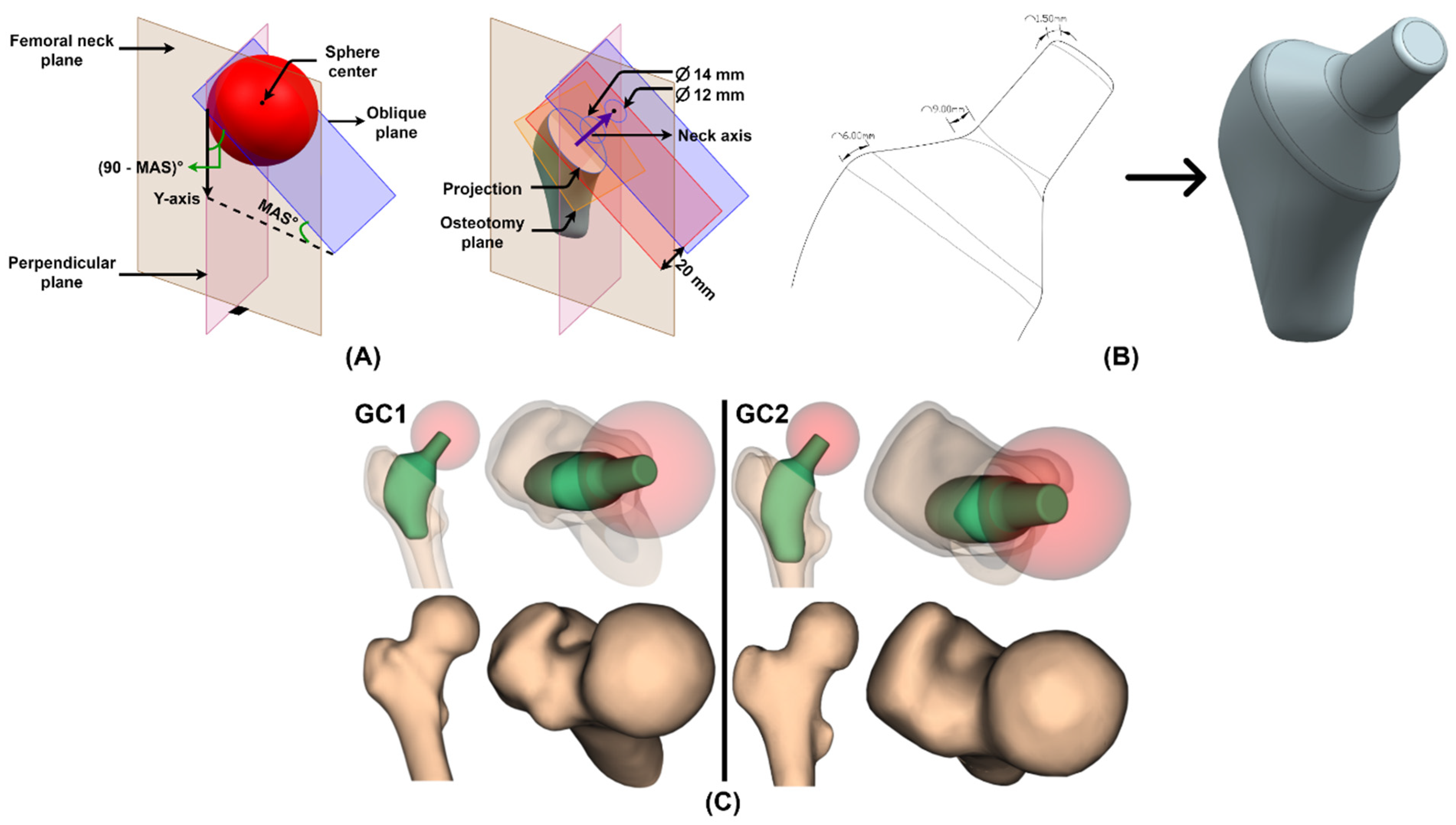
2.4.1. Osteotomy
2.4.2. Insertion
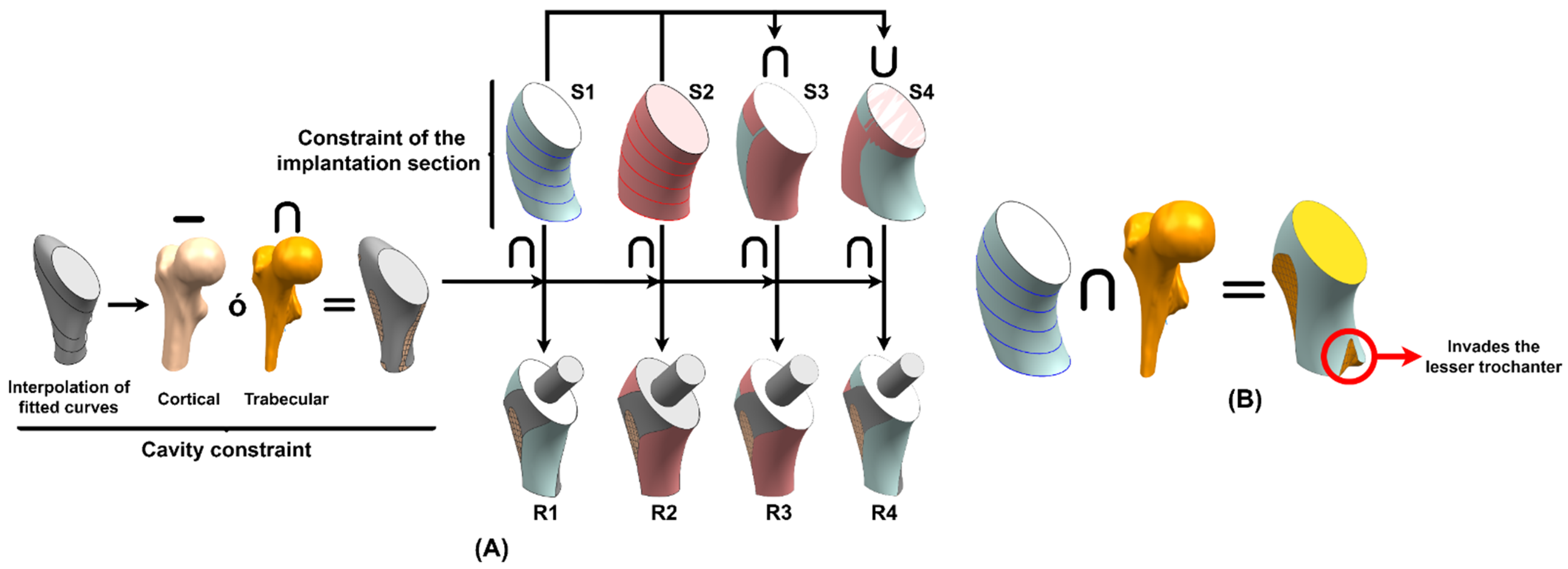
2.4.3. Implantability
2.4.4. Stem
2.4.5. Neck and Receiving Taper
2.5. Finite Element Model
2.5.1. Mesh
2.5.2. Bone Properties
2.5.3. Stem Properties
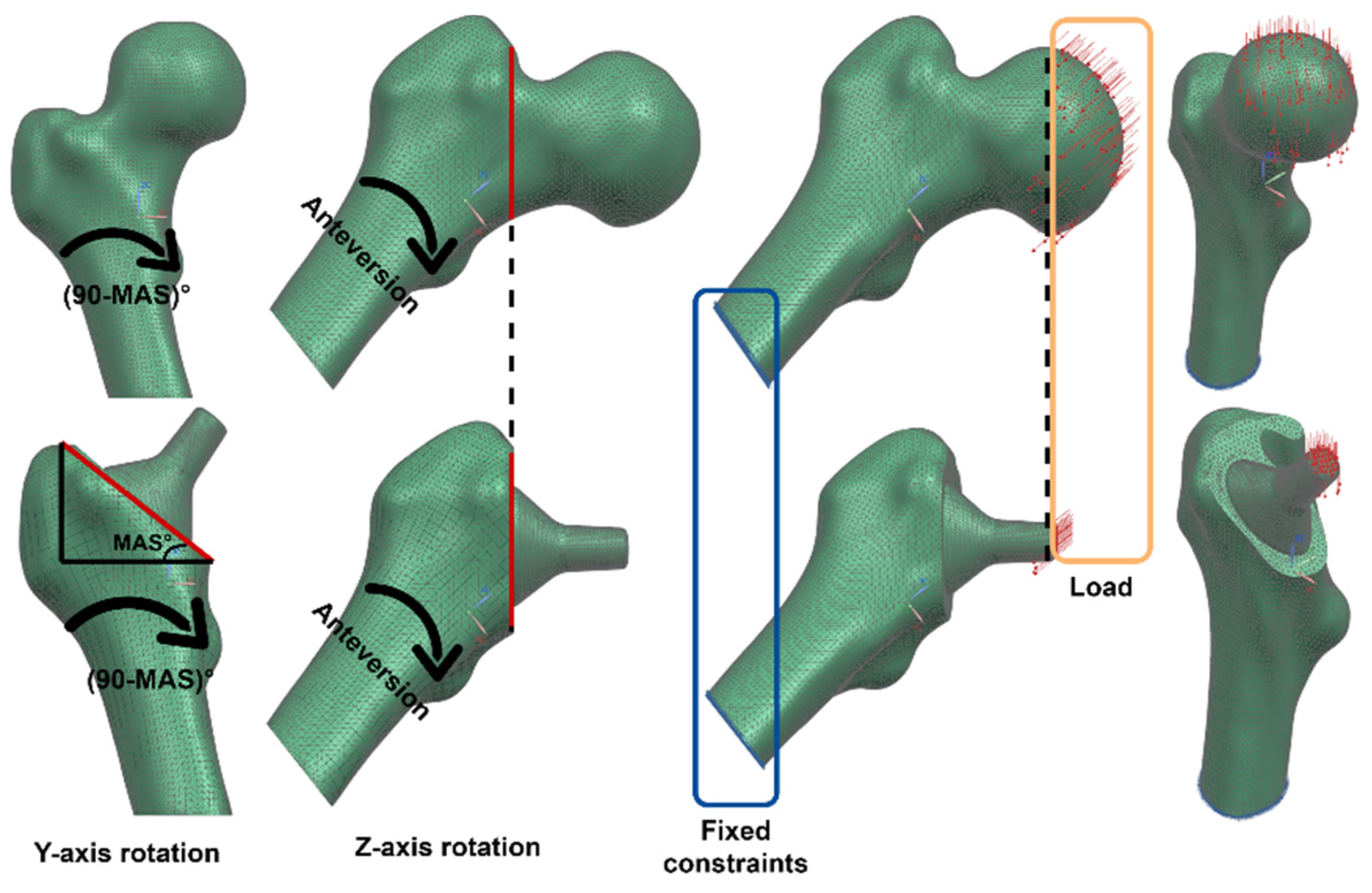
2.5.4. Boundary Conditions
2.5.5. Postprocessing
3. Results and Discussion
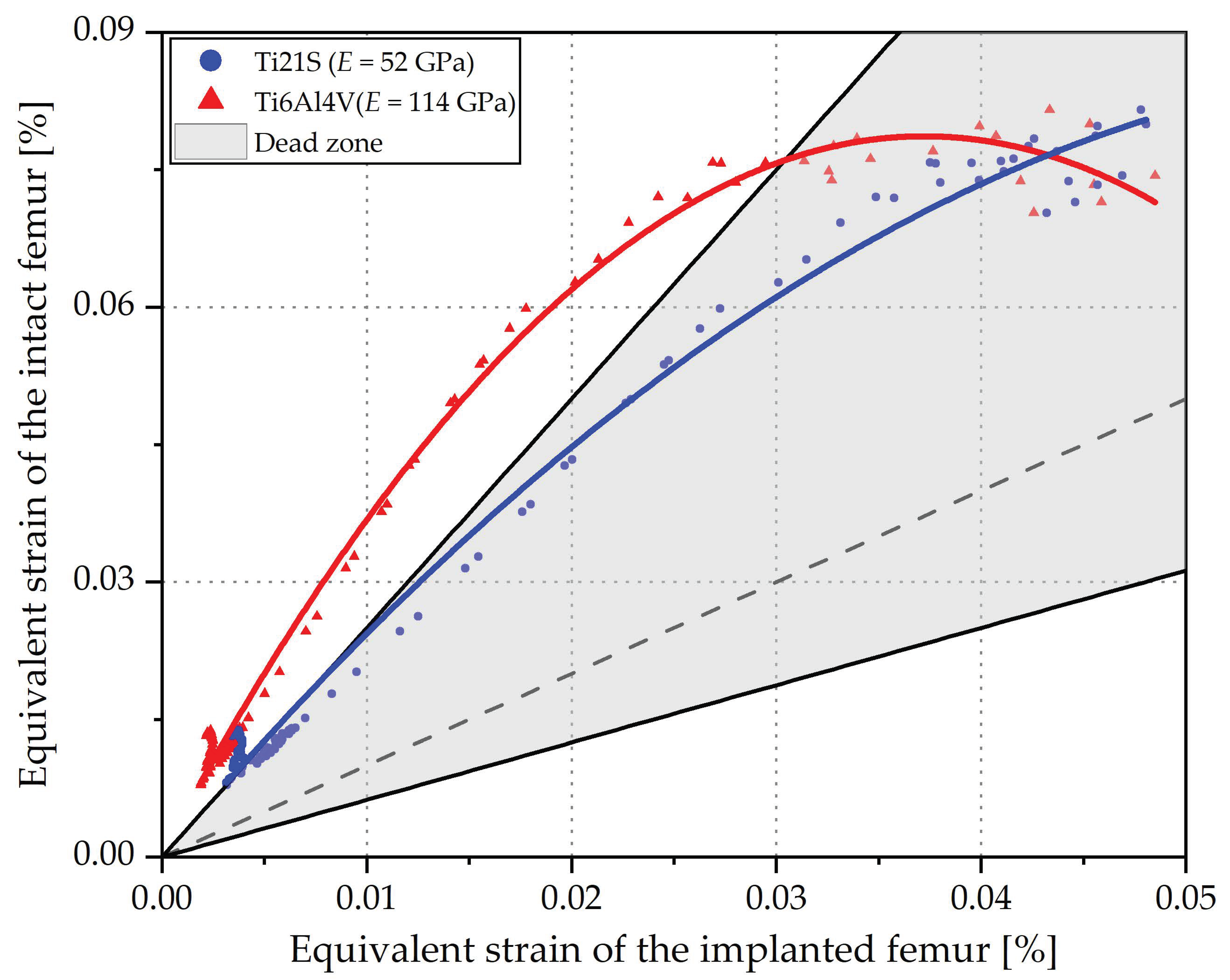
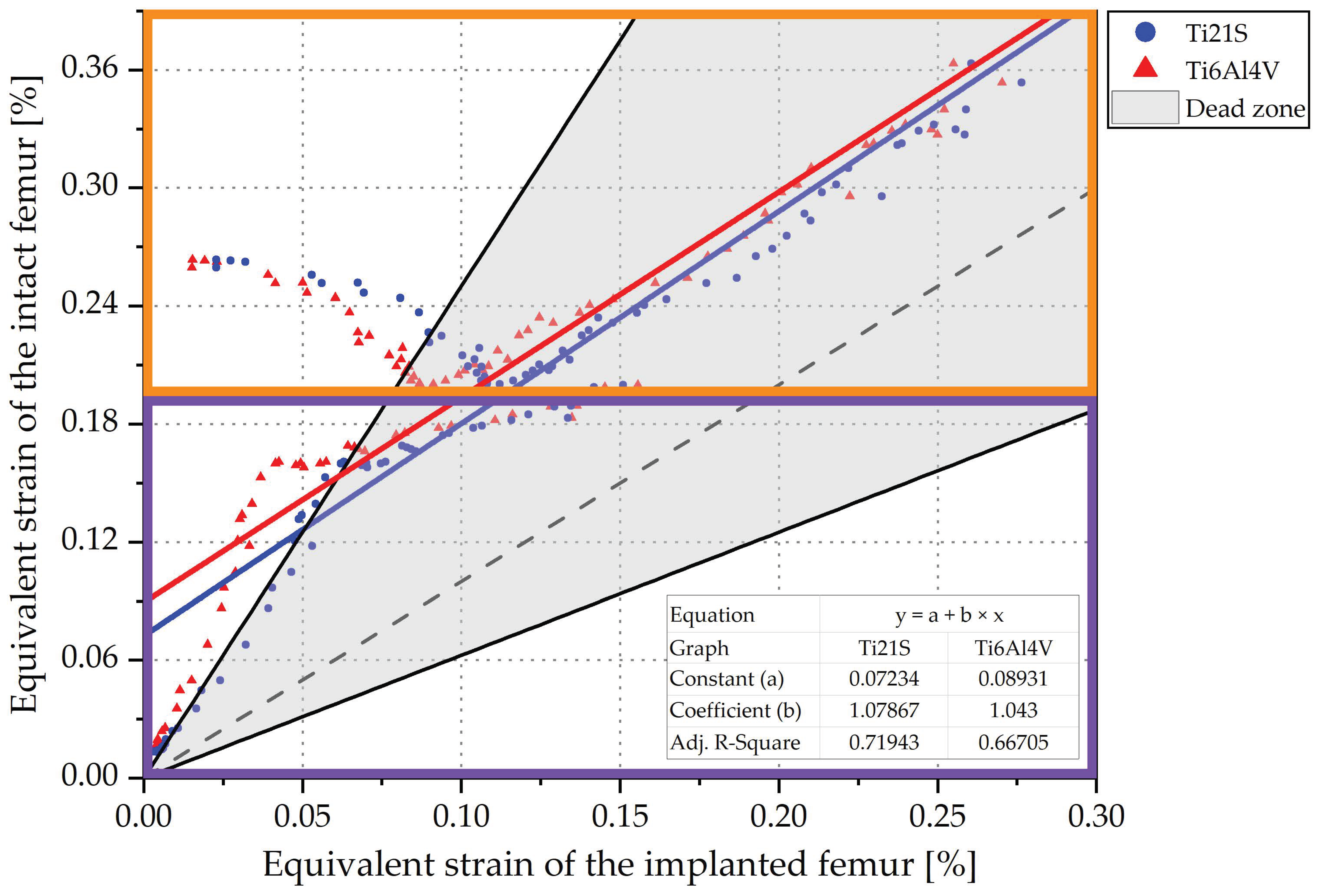
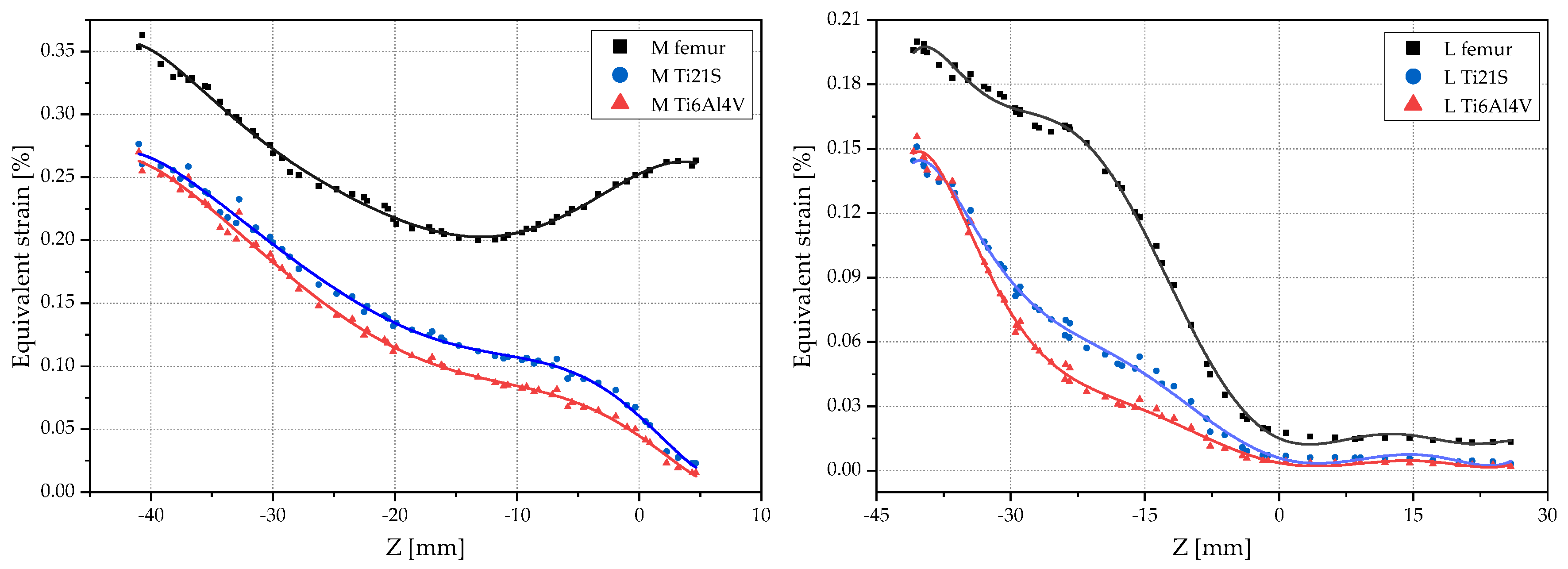
3.1. Remodeling Curve and Regression Graph
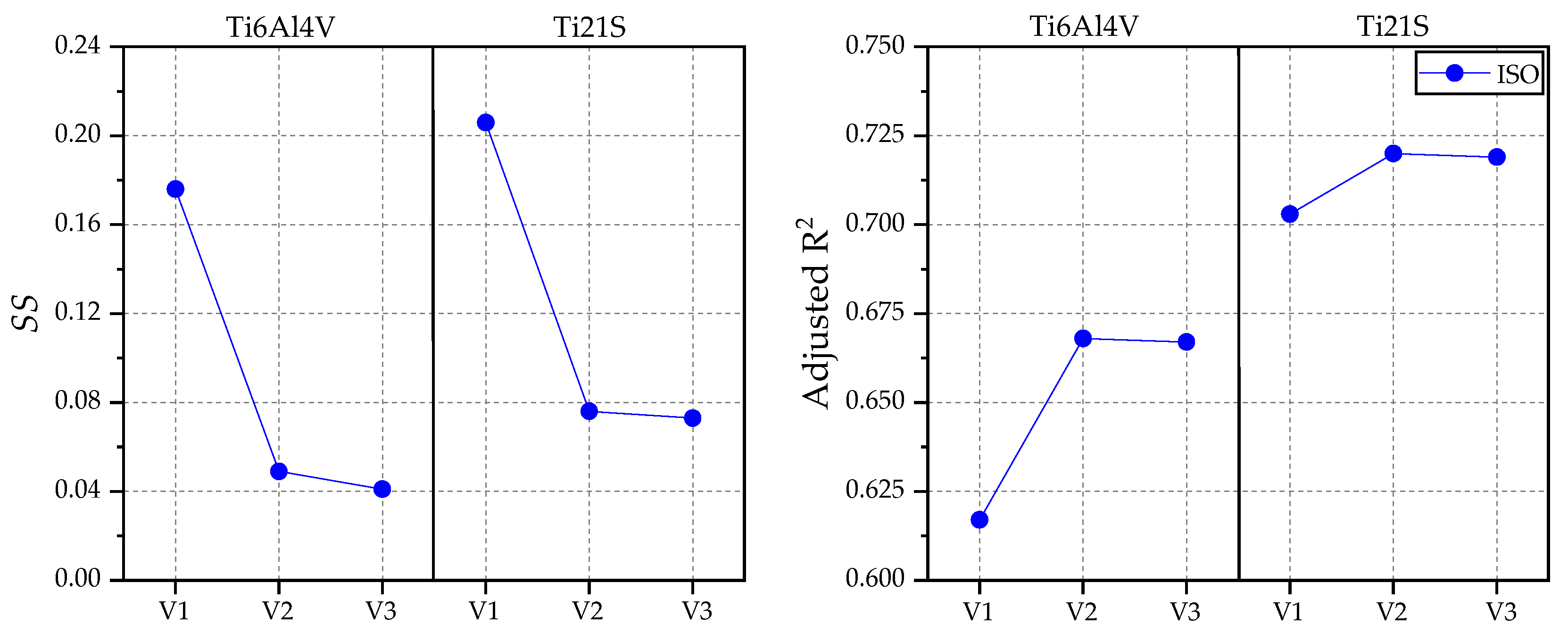
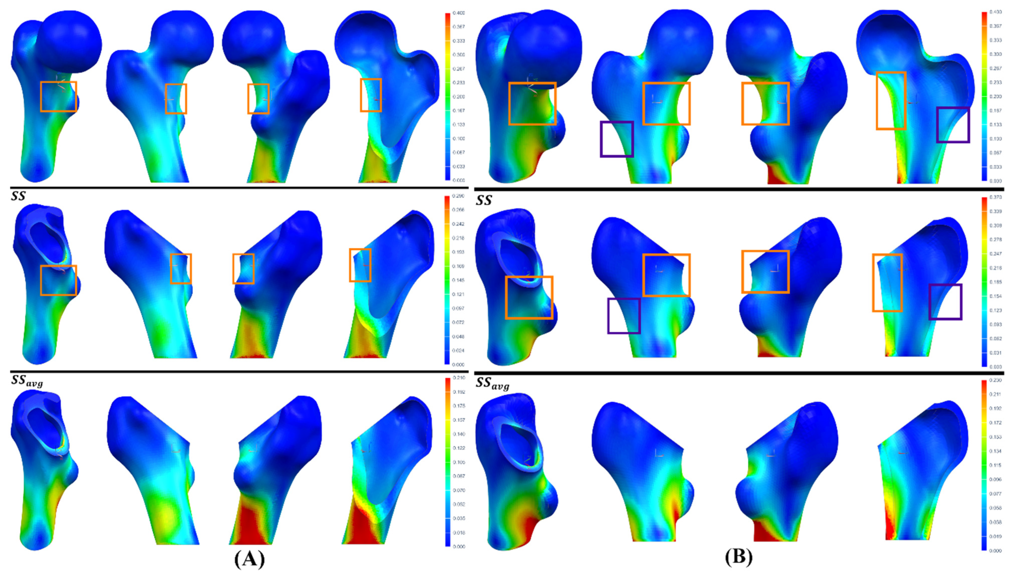
3.2. Analysis
4. Limitations and Future Proposals
4.1. Limitations of the Study
4.2. Future Research Proposals
5. Conclusions
Author Contributions
Funding
Institutional Review Board Statement
Informed Consent Statement
Data Availability Statement
Acknowledgments
Conflicts of Interest
References
- Ojeda, C. Estudio de La Influencia de Estabilidad Primaria En El Diseño de Vástagos de Prótesis Femorales Personalizadas: Aplicación a Paciente Específico. Ph.D. Thesis, Universidad Politécnica de Madrid, Madrid, Spain, 2009. [Google Scholar]
- Santori, N.; Lucidi, M.; Santori, F.S. Proximal Load Transfer with a Stemless Uncemented Femoral Implant. J. Orthop. Traumatol. 2006, 7, 154–160. [Google Scholar] [CrossRef]
- Fetto, J.F.; Bettinger, P.; Austin, K. Reexamination of Hip Biomechanics during Unilateral Stance. Am. J. Orthop. Belle Mead NJ 1995, 24, 605–612. [Google Scholar] [PubMed]
- Duque Morán, J.; Navarro Navarro, R.; Navarro García, R.; Ruiz Caballero, J.A. Biomecánica de La Protesis Total de Cadera: Cementadas y No Cementadas. Canar. Médica Quirúrgica 2011, 9, 32–47. [Google Scholar]
- Ridzwan, M.I.Z.; Shuib, S.; Hassan, A.Y.; Shokri, A.A.; Mohamad Ib, M.N. Problem of Stress Shielding and Improvement to the Hip Implant Designs: A Review. J. Med. Sci. 2007, 7, 460–467. [Google Scholar] [CrossRef]
- Swiontkowski, M.F.; Winquist, R.A.; Hansen, S.T. Fractures of the Femoral Neck in Patients between the Ages of Twelve and Forty-Nine Years. J. Bone Jt. Surg. 1984, 66, 837–846. [Google Scholar] [CrossRef]
- Sornay-Rendu, E.; Boutroy, S.; Munoz, F.; Delmas, P.D. Alterations of Cortical and Trabecular Architecture Are Associated with Fractures in Postmenopausal Women, Partially Independent of Decreased BMD Measured by DXA: The OFELY Study. J. Bone Miner. Res. 2007, 22, 425–433. [Google Scholar] [CrossRef]
- Garden, R.S. Low-Angle Fixation in Fractures of the Femoral Neck. J. Bone Jt. Surg. Br. 1961, 43-B, 647–663. [Google Scholar] [CrossRef]
- Santori, N.; Albanese, C.V.; Learmonth, I.D.; Santori, F.S. Bone Preservation with a Conservative Metaphyseal Loading Implant. Hip Int. 2006, 16, 16–21. [Google Scholar] [CrossRef]
- Jasty, M.; Krushell, R.; Zalenski, E.; O’Connor, D.; Sedlacek, R.; Harris, W. The Contribution of the Nonporous Distal Stem to the Stability of Proximally Porous-Coated Canine Femoral Components. J. Arthroplast. 1993, 8, 33–41. [Google Scholar] [CrossRef]
- Zuley, M.L.; Jarosz, R.; Drake, B.F.; Rancilio, D.; Klim, A.; Rieger-Christ, K.; Lemmerman, J. Radiology Data from The Cancer Genome Atlas Prostate Adenocarcinoma [TCGA-PRAD] Collection. Cancer Imaging Arch. 2016. [Google Scholar] [CrossRef]
- Yorke, A.A.; McDonald, G.C.; Solis, D.; Guerrero, T. Pelvic Reference Data. Cancer Imaging Arch. 2019. [Google Scholar] [CrossRef]
- Rinaldi, G.; Capitani, D.; Maspero, F.; Scita, V. Mid-Term Results with a Neck-Preserving Femoral Stem for Total Hip Arthroplasty. HIP Int. 2018, 28, 28–34. [Google Scholar] [CrossRef]
- Sabatini, A.L.; Goswami, T. Hip Implants VII: Finite Element Analysis and Optimization of Cross-Sections. Mater. Des. 2008, 29, 1438–1446. [Google Scholar] [CrossRef]
- Fitzgibbon, A.; Pilu, M.; Fisher, R.B. Direct Least Square Fitting of Ellipses. IEEE Trans. Pattern Anal. Mach. Intell. 1999, 21, 476–480. [Google Scholar] [CrossRef]
- Paton, K. Conic Sections in Chromosome Analysis. Pattern Recognit. 1970, 2, 39–51. [Google Scholar] [CrossRef]
- Cruz-Díaz, C. Ajuste Robusto de Múltiples Elipses Usando Algoritmos Genéticos. Master’s Thesis, Instituto Politécnico Nacional, Mexico City, México, 2012. [Google Scholar]
- Solórzano, W.; Ojeda, C.; Diaz Lantada, A. Biomechanical Study of Proximal Femur for Designing Stems for Total Hip Replacement. Appl. Sci. 2020, 10, 4208. [Google Scholar] [CrossRef]
- Carter, L.W.; Stovall, D.O.; Young, T.R. Determination of Accuracy of Preoperative Templating of Noncemented Femoral Prostheses. J. Arthroplast. 1995, 10, 507–513. [Google Scholar] [CrossRef]
- Crooijmans, H.J.A.; Laumen, A.M.R.P.; van Pul, C.; van Mourik, J.B.A. A New Digital Preoperative Planning Method for Total Hip Arthroplasties. Clin. Orthop. 2009, 467, 909–916. [Google Scholar] [CrossRef]
- Fottner, A.; Peter, C.V.; Schmidutz, F.; Wanke-Jellinek, L.; Schröder, C.; Mazoochian, F.; Jansson, V. Biomechanical Evaluation of Different Offset Versions of a Cementless Hip Prosthesis by 3-Dimensional Measurement of Micromotions. Clin. Biomech. 2011, 26, 830–835. [Google Scholar] [CrossRef] [PubMed]
- Viceconti, M.; Lattanzi, R.; Antonietti, B.; Paderni, S.; Olmi, R.; Sudanese, A.; Toni, A. CT-Based Surgical Planning Software Improves the Accuracy of Total Hip Replacement Preoperative Planning. Med. Eng. Phys. 2003, 25, 371–377. [Google Scholar] [CrossRef]
- Toth, K.; Sohar, G. Short-Stem Hip Arthroplasty. In Arthroplasty—Update; Kinov, P., Ed.; InTech: London, UK, 2013; ISBN 978-953-51-0995-2. [Google Scholar]
- Wen-ming, X.; Ai-min, W.; Qi, W.; Chang-Hua, L.; Jian-fei, Z.; Fang-fang, X. An Integrated CAD/CAM/Robotic Milling Method for Custom Cementless Femoral Prostheses. Med. Eng. Phys. 2015, 37, 911–915. [Google Scholar] [CrossRef] [PubMed]
- Baharuddin, M.Y.; Salleh, S.-H.; Zulkifly, A.H.; Lee, M.H.; Mohd Noor, A. Morphological Study of the Newly Designed Cementless Femoral Stem. BioMed Res. Int. 2014, 2014, 692328. [Google Scholar] [CrossRef] [PubMed]
- Wang, Z.; Li, H.; Zhou, Y.; Deng, W. Three-Dimensional Femoral Morphology in Hartofilakidis Type C Developmental Dysplastic Hips and the Implications for Total Hip Arthroplasty. Int. Orthop. 2020, 44, 1935–1942. [Google Scholar] [CrossRef]
- Zhang, R.-Y.; Su, X.-Y.; Zhao, J.-X.; Li, J.-T.; Zhang, L.-C.; Tang, P.-F. Three-Dimensional Morphological Analysis of the Femoral Neck Torsion Angle—An Anatomical Study. J. Orthop. Surg. 2020, 15, 192. [Google Scholar] [CrossRef] [PubMed]
- Gilligan, I.; Chandraphak, S.; Mahakkanukrauh, P. Femoral Neck-Shaft Angle in Humans: Variation Relating to Climate, Clothing, Lifestyle, Sex, Age and Side. J. Anat. 2013, 223, 133–151. [Google Scholar] [CrossRef]
- Gusmão, L.C.B.D.; Sousa Rodrigues, C.F.D.; Martins, J.S.; Silva, A.J.D. Ángulo de Inclinación Del Fémur En El Hombre y Su Relación Con La Coxa Vara y La Coxa Valga. Int. J. Morphol. 2011, 29, 389–392. [Google Scholar] [CrossRef]
- Houcke, J.; Khanduja, V.; Pattyn, C.; Audenaert, E. The History of Biomechanics in Total Hip Arthroplasty. Indian J. Orthop. 2017, 51, 359–367. [Google Scholar] [CrossRef]
- Charles, M.N.; Bourne, R.B.; Davey, J.R.; Greenwald, A.S.; Morrey, B.F.; Rorabeck, C.H. Soft-Tissue Balancing of the Hip: The Role of Femoral Offset Restoration. Instr. Course Lect. 2005, 54, 131–141. [Google Scholar] [CrossRef]
- Widmer, K.-H.; Majewski, M. The Impact of the CCD-Angle on Range of Motion and Cup Positioning in Total Hip Arthroplasty. Clin. Biomech. 2005, 20, 723–728. [Google Scholar] [CrossRef]
- Yadav, P.; Shefelbine, S.J.; Gutierrez-Farewik, E.M. Effect of Growth Plate Geometry and Growth Direction on Prediction of Proximal Femoral Morphology. J. Biomech. 2016, 49, 1613–1619. [Google Scholar] [CrossRef]
- Lewinnek, G.E.; Lewis, J.L.; Tarr, R.; Compere, C.L.; Zimmerman, J.R. Dislocations after Total Hip-Replacement Arthroplasties. J. Bone Jt. Surg. 1978, 60, 217–220. [Google Scholar] [CrossRef]
- Matovinović, D.; Nemec, B.; Gulan, G.; Sestan, B.; Ravlić-Gulan, J. Comparison in Regression of Femoral Neck Anteversion in Children with Normal, Intoeing and Outtoeing Gait—Prospective Study. Coll. Antropol. 1998, 22, 525–532. [Google Scholar]
- Svenningsen, S.; Apalset, K.; Terjesen, T.; Anda, S. Regression of Femoral Anteversion: A Prospective Study of Intoeing Children. Acta Orthop. Scand. 1989, 60, 170–173. [Google Scholar] [CrossRef]
- Bergmann, G.; Graichen, F.; Rohlmann, A. Hip Joint Loading during Walking and Running, Measured in Two Patients. J. Biomech. 1993, 26, 969–990. [Google Scholar] [CrossRef]
- Hauptfleisch, J.; Glyn-Jones, S.; Beard, D.J.; Gill, H.S.; Murray, D.W. The Premature Failure of the Charnley Elite-Plus Stem: A CONFIRMATION OF RSA PREDICTIONS. J. Bone Jt. Surg. Br. 2006, 88-B, 179–183. [Google Scholar] [CrossRef]
- Heller, M.O.; Bergmann, G.; Deuretzbacher, G.; Claes, L.; Haas, N.P.; Duda, G.N. Influence of Femoral Anteversion on Proximal Femoral Loading: Measurement and Simulation in Four Patients. Clin. Biomech. 2001, 16, 644–649. [Google Scholar] [CrossRef]
- Widmer, K.-H.; Zurfluh, B. Compliant Positioning of Total Hip Components for Optimal Range of Motion. J. Orthop. Res. 2004, 22, 815–821. [Google Scholar] [CrossRef] [PubMed]
- Dorr, L.D.; Malik, A.; Dastane, M.; Wan, Z. Combined Anteversion Technique for Total Hip Arthroplasty. Clin. Orthop. 2009, 467, 119–127. [Google Scholar] [CrossRef]
- Matsushita, A.; Nakashima, Y.; Jingushi, S.; Yamamoto, T.; Kuraoka, A.; Iwamoto, Y. Effects of the Femoral Offset and the Head Size on the Safe Range of Motion in Total Hip Arthroplasty. J. Arthroplast. 2009, 24, 646–651. [Google Scholar] [CrossRef] [PubMed]
- Chandler, D.R.; Glousman, R.; Hull, D.; Mcguire, P.J.; Clarke, I.C.; Sarmiento, A. Prosthetic Hip Range of Motion and Impingement: The Effects of Head and Neck Geometry. Clin. Orthop. 1982, 166, 284–291. [Google Scholar] [CrossRef]
- Berstock, J.R.; Hughes, A.M.; Lindh, A.M.; Smith, E.J. A Radiographic Comparison of Femoral Offset after Cemented and Cementless Total Hip Arthroplasty. HIP Int. 2014, 24, 582–586. [Google Scholar] [CrossRef]
- Sakalkale, D.P.; Sharkey, P.F.; Eng, K.; Hozack, W.J.; Rothman, R.H. Effect of Femoral Component Offset on Polyethylene Wear in Total Hip Arthroplasty. Clin. Orthop. 2001, 388, 125–134. [Google Scholar] [CrossRef]
- Kheir, M.M.; Drayer, N.J.; Chen, A.F. An Update on Cementless Femoral Fixation in Total Hip Arthroplasty. J. Bone Jt. Surg. 2020, 102, 1646–1661. [Google Scholar] [CrossRef]
- Gómez-García, F.; Fernández-Fairen, M.; Espinosa-Mendoza, R.L. A Proposal for the Study of Cementless Short-Stem Hip Prostheses. Acta Ortop. Mex. 2016, 30, 204–215. [Google Scholar]
- Dimitriou, D.; Tsai, T.-Y.; Kwon, Y.-M. The Effect of Femoral Neck Osteotomy on Femoral Component Position of a Primary Cementless Total Hip Arthroplasty. Int. Orthop. 2015, 39, 2315–2321. [Google Scholar] [CrossRef]
- Michel, M.C.; Witschger, P. MicroHip: A Minimally Invasive Procedure for Total Hip Replacement Surgery Using a Modified Smith-Peterson Approach. Ortop. Traumatol. Rehabil. 2007, 9, 46–51. [Google Scholar] [PubMed]
- Gombár, C.; Janositz, G.; Friebert, G.; Sisák, K. The DePuy ProximaTM Short Stem for Total Hip Arthroplasty—Excellent Outcome at a Minimum of 7 Years. J. Orthop. Surg. 2019, 27, 2309499019838668. [Google Scholar] [CrossRef] [PubMed]
- Morlock, M.M.; Hube, R.; Wassilew, G.; Prange, F.; Huber, G.; Perka, C. Taper Corrosion: A Complication of Total Hip Arthroplasty. EFORT Open Rev. 2020, 5, 776–784. [Google Scholar] [CrossRef] [PubMed]
- Wang, S.; Zhou, X.; Liu, L.; Shi, Z.; Hao, Y. On the Design and Properties of Porous Femoral Stems with Adjustable Stiffness Gradient. Med. Eng. Phys. 2020, 81, 30–38. [Google Scholar] [CrossRef]
- Brown, T.D.; Ferguson, A.B. Mechanical Property Distributions in the Cancellous Bone of the Human Proximal Femur. Acta Orthop. Scand. 1980, 51, 429–437. [Google Scholar] [CrossRef]
- Rho, J.Y.; Hobatho, M.C.; Ashman, R.B. Relations of Mechanical Properties to Density and CT Numbers in Human Bone. Med. Eng. Phys. 1995, 17, 347–355. [Google Scholar] [CrossRef]
- Keyak, J.H.; Kaneko, T.S.; Tehranzadeh, J.; Skinner, H.B. Predicting Proximal Femoral Strength Using Structural Engineering Models. Clin. Orthop. Relat. Res. 2005, 437, 219–228. [Google Scholar] [CrossRef]
- Schileo, E.; Dall’Ara, E.; Taddei, F.; Malandrino, A.; Schotkamp, T.; Baleani, M.; Viceconti, M. An Accurate Estimation of Bone Density Improves the Accuracy of Subject-Specific Finite Element Models. J. Biomech. 2008, 41, 2483–2491. [Google Scholar] [CrossRef]
- Pithioux, M. Lois de comportement et modèles de rupture des os longs en accidentologie. Ph.D. Thesis, Université de la Méditerranée, Marseille, Francia, 2000. [Google Scholar]
- Peng, L.; Bai, J.; Zeng, X.; Zhou, Y. Comparison of Isotropic and Orthotropic Material Property Assignments on Femoral Finite Element Models under Two Loading Conditions. Med. Eng. Phys. 2006, 28, 227–233. [Google Scholar] [CrossRef]
- Hernandez, C.J. Chapter A2 Cancellous Bone. In Handbook of Biomaterial Properties; Murphy, W., Black, J., Hastings, G., Eds.; Springer: New York, NY, USA, 2016; pp. 15–21. ISBN 978-1-4939-3303-7. [Google Scholar]
- Wirtz, D.C.; Schiffers, N.; Pandorf, T.; Radermacher, K.; Weichert, D.; Forst, R. Critical Evaluation of Known Bone Material Properties to Realize Anisotropic FE-Simulation of the Proximal Femur. J. Biomech. 2000, 33, 1325–1330. [Google Scholar] [CrossRef]
- Yang, H.-S.; Guo, T.-T.; Wu, J.-H.; Ma, X. Inhomogeneous Material Property Assignment and Orientation Definition of Transverse Isotropy of Femur. J. Biomed. Sci. Eng. 2009, 2, 419–424. [Google Scholar] [CrossRef][Green Version]
- Rickert, D.; Lendlein, A.; Peters, I.; Moses, M.A.; Franke, R.-P. Biocompatibility Testing of Novel Multifunctional Polymeric Biomaterials for Tissue Engineering Applications in Head and Neck Surgery: An Overview. Eur. Arch. Otorhinolaryngol. 2006, 263, 215–222. [Google Scholar] [CrossRef] [PubMed]
- Becker, E.L.; Landau, I. International Dictionary of Medicine and Biology. J. Clin. Eng. 1986, 11, 134. [Google Scholar] [CrossRef]
- Sam Froes, F.H. Titanium for Medical and Dental Applications—An Introduction. In Titanium in Medical and Dental Applications; Elsevier: Amsterdam, The Netherlands, 2018; pp. 3–21. ISBN 978-0-12-812456-7. [Google Scholar]
- Choroszyński, M.; Choroszyński, M.R.; Skrzypek, S.J. Biomaterials for Hip Implants—Important Considerations Relating to the Choice of Materials. Bio-Algorithms Med-Syst. 2017, 13, 133–145. [Google Scholar] [CrossRef]
- Okazaki, Y.; Gotoh, E. Comparison of Metal Release from Various Metallic Biomaterials in Vitro. Biomaterials 2005, 26, 11–21. [Google Scholar] [CrossRef] [PubMed]
- Browne, M.; Gregson, P.J. Surface Modification of Titanium Alloy Implants. Biomaterials 1994, 15, 894–898. [Google Scholar] [CrossRef]
- Pellizzari, M.; Jam, A.; Tschon, M.; Fini, M.; Lora, C.; Benedetti, M. A 3D-Printed Ultra-Low Young’s Modulus β-Ti Alloy for Biomedical Applications. Materials 2020, 13, 2792. [Google Scholar] [CrossRef] [PubMed]
- Petrovic, V.; Vicente Haro Gonzalez, J.; Jordá Ferrando, O.; Delgado Gordillo, J.; Ramón Blasco Puchades, J.; Portolés Griñan, L. Additive Layered Manufacturing: Sectors of Industrial Application Shown through Case Studies. Int. J. Prod. Res. 2011, 49, 1061–1079. [Google Scholar] [CrossRef]
- Horn, T.J.; Harrysson, O.L.A. Overview of Current Additive Manufacturing Technologies and Selected Applications. Sci. Prog. 2012, 95, 255–282. [Google Scholar] [CrossRef] [PubMed]
- Markwardt, J.; Friedrichs, J.; Werner, C.; Davids, A.; Weise, H.; Lesche, R.; Weber, A.; Range, U.; Meißner, H.; Lauer, G.; et al. Experimental Study on the Behavior of Primary Human Osteoblasts on Laser-Cused Pure Titanium Surfaces: Human Osteoblasts on Laser—Cused Titanium. J. Biomed. Mater. Res. A 2014, 102, 1422–1430. [Google Scholar] [CrossRef]
- Ponader, S.; Von Wilmowsky, C.; Widenmayer, M.; Lutz, R.; Heinl, P.; Körner, C.; Singer, R.F.; Nkenke, E.; Neukam, F.W.; Schlegel, K.A. In Vivo Performance of Selective Electron Beam-Melted Ti-6Al-4V Structures. J. Biomed. Mater. Res. Part A 2010, 92, 56–62. [Google Scholar] [CrossRef]
- ASTM International. ASTM International ASTM F136-08: Standard Specification for Wrought Titanium-6 Aluminum-4 Vanadium ELI (Extra Low Interstitial) Alloy for Surgical Implant Applications (UNS R56401); ASTM International: West Conshohocken, PA, USA, 2008. [Google Scholar]
- Bergmann, G.; Bender, A.; Dymke, J.; Duda, G.; Damm, P. Standardized Loads Acting in Hip Implants. PLoS ONE 2016, 11, e0155612. [Google Scholar] [CrossRef]
- International Organization for Standardization (ISO). International Standard ISO 7206-4 Implants for Surgery-Partial and Total Hip Joint Prostheses, Part 4: Determination of Endurance Properties and Performance of Stemmed Femoral Components; International Organization for Standardization (ISO): Geneva, Switzerland, 2010.
- Wolff, J. Das Gesetz der Transformation der Knochen. DMW—Dtsch. Med. Wochenschr. 1893, 19, 1222–1224. [Google Scholar] [CrossRef]
- Frost, H.M. Bone’s Mechanostat: A 2003 Update. Anat. Rec. 2003, 275A, 1081–1101. [Google Scholar] [CrossRef]
- Mikić, B.; Carter, D.R. Bone Strain Gage Data and Theoretical Models of Functional Adaptation. J. Biomech. 1995, 28, 465–469. [Google Scholar] [CrossRef]
- Turner, A.W.L.; Gillies, R.M.; Sekel, R.; Morris, P.; Bruce, W.; Walsh, W.R. Computational Bone Remodelling Simulations and Comparisons with DEXA Results. J. Orthop. Res. 2005, 23, 705–712. [Google Scholar] [CrossRef]
- Yan, S.G.; Chevalier, Y.; Liu, F.; Hua, X.; Schreiner, A.; Jansson, V.; Schmidutz, F. Metaphyseal Anchoring Short Stem Hip Arthroplasty Provides a More Physiological Load Transfer: A Comparative Finite Element Analysis Study. J. Orthop. Surg. 2020, 15, 498. [Google Scholar] [CrossRef] [PubMed]
- Yamako, G.; Chosa, E.; Totoribe, K.; Hanada, S.; Masahashi, N.; Yamada, N.; Itoi, E. In-Vitro Biomechanical Evaluation of Stress Shielding and Initial Stability of a Low-Modulus Hip Stem Made of β Type Ti-33.6Nb-4Sn Alloy. Med. Eng. Phys. 2014, 36, 1665–1671. [Google Scholar] [CrossRef] [PubMed]
- Srinivasan, A.; Jung, E.; Levine, B.R. Modularity of the Femoral Component in Total Hip Arthroplasty. J. Am. Acad. Orthop. Surg. 2012, 20, 214–222. [Google Scholar] [CrossRef] [PubMed]
- Boccaccio, A.; Uva, A.E.; Fiorentino, M.; Monno, G.; Ballini, A.; Desiate, A. Optimal Load for Bone Tissue Scaffolds with an Assigned Geometry. Int. J. Med. Sci. 2018, 15, 16–22. [Google Scholar] [CrossRef] [PubMed]


| Properties | Cortical Bone | Trabecular Bone | ||
|---|---|---|---|---|
| GC1 | GC2 | GC1 | GC2 | |
| 1458 | 1197 | 779 | 745 | |
| 1.69 | 1.41 | 0.96 | 0.93 | |
| (MPa) | 9140.76 | 6534.52 | 5363.09 | 4993.1 |
| (MPa) | 9140.76 | 6534.52 | ||
| (MPa) | 15,234.61 | 10,890.87 | ||
| (MPa) | 3264.56 | 2333.76 | 2062.73 | 1920.42 |
| (MPa) | 3808.65 | 2722.72 | ||
| (MPa) | 3808.65 | 2722.72 | ||
| 0.4 | 0.4 | 0.3 | 0.3 | |
| 0.25 | 0.25 | |||
| 0.25 | 0.25 | |||
| Properties | Ti6Al4V ELI [73] | Ti21S [68] |
|---|---|---|
| (GPa) | 114 | 52 |
| (GPa) | 42.5 | 19.6 |
| 0.34 | 0.33 | |
| (MPa) | 795 | 709 |
| Jogging [74] | ISO [75] | |
|---|---|---|
| (N) | −884.8 | - |
| (N) | −15 | - |
| (N) | −3222 | −2300 |
| (Nm) | −0.69 | - |
| (Nm) | 0.76 | - |
| (Nm) | 0.09 | - |
| Element | |||
|---|---|---|---|
| 1 | 0.11 | 0.05 | 0.545 |
| 2 | 0.075 | 0.13 | −0.733 |
| 3 | 0.5 | 0.3 | 0.4 |
| 4 | 0.08 | 0.1 | −0.25 |
| Average | 7.875) | 7.75) | 0.016) |
| Ti6Al4V | Ti21S | ||||||
|---|---|---|---|---|---|---|---|
| V1 | V2 | V3 | V1 | V2 | V3 | ||
| ISO | Adjusted R2 | 0.759 | 0.78 | 0.78 | 0.793 | 0.804 | 0.804 |
| Constant | 0.024 | 0.023 | 0.023 | 0.017 | 0.017 | 0.017 | |
| Coefficient | 1.511 | 1.41 | 1.412 | 1.468 | 1.397 | 1.399 | |
| 0.338 | 0.291 | 0.292 | 0.319 | 0.284 | 0.285 | ||
| 0.574 | 0.535 | 0.533 | 0.496 | 0.473 | 0.47 | ||
| Jogging | Adjusted R2 | 0.642 | 0.683 | 0.683 | 0.677 | 0.701 | 0.701 |
| Constant | 0.013 | 0.013 | 0.013 | 0.008 | 0.008 | 0.008 | |
| Coefficient | 1.792 | 1.706 | 1.708 | 1.735 | 1.663 | 1.664 | |
| 0.442 | 0.414 | 0.415 | 0.424 | 0.399 | 0.399 | ||
| 0.605 | 0.58 | 0.578 | 0.525 | 0.506 | 0.504 | ||
| Ti6Al4V | Ti21S | |||||
|---|---|---|---|---|---|---|
| V1 | V2 | V3 | V1 | V2 | V3 | |
| Adjusted R2 | 0.617 | 0.668 | 0.667 | 0.703 | 0.72 | 0.719 |
| Constant | 0.097 | 0.09 | 0.089 | 0.073 | 0.073 | 0.072 |
| Coefficient | 1.213 | 1.052 | 1.043 | 1.26 | 1.082 | 1.079 |
| 0.176 | 0.049 | 0.041 | 0.206 | 0.076 | 0.073 | |
| 0.611 | 0.512 | 0.505 | 0.521 | 0.443 | 0.437 | |
Publisher’s Note: MDPI stays neutral with regard to jurisdictional claims in published maps and institutional affiliations. |
© 2022 by the authors. Licensee MDPI, Basel, Switzerland. This article is an open access article distributed under the terms and conditions of the Creative Commons Attribution (CC BY) license (https://creativecommons.org/licenses/by/4.0/).
Share and Cite
Solórzano-Requejo, W.; Ojeda, C.; Díaz Lantada, A. Innovative Design Methodology for Patient-Specific Short Femoral Stems. Materials 2022, 15, 442. https://doi.org/10.3390/ma15020442
Solórzano-Requejo W, Ojeda C, Díaz Lantada A. Innovative Design Methodology for Patient-Specific Short Femoral Stems. Materials. 2022; 15(2):442. https://doi.org/10.3390/ma15020442
Chicago/Turabian StyleSolórzano-Requejo, William, Carlos Ojeda, and Andrés Díaz Lantada. 2022. "Innovative Design Methodology for Patient-Specific Short Femoral Stems" Materials 15, no. 2: 442. https://doi.org/10.3390/ma15020442
APA StyleSolórzano-Requejo, W., Ojeda, C., & Díaz Lantada, A. (2022). Innovative Design Methodology for Patient-Specific Short Femoral Stems. Materials, 15(2), 442. https://doi.org/10.3390/ma15020442