
Is Wood a Material? Taking the Size Effect Seriously


Abstract
:1. Introduction
2. The Classical Understanding of Elasticity
“We might consider a wire as composed of a great number of minute threads, extending through its length, and closely connected together; if we twisted such a wire, the external threads would be extended, and in order to preserve the equilibrium, the internal ones would be contracted…”
3. Problems with the Application of Elasticity Theory to Wood
4. Problems in Discerning Trends in the Strength of Wood
5. Size Effect Theories
“Predicting yield of structural members under complex loading conditions is a difficult task for the engineer. Complex loading often results in the structural members being stressed biaxially or even triaxially, whereas yield strength data are usually only available for tests conducted in uniaxial (tensile or compressive) or torsional stress states. The test specimens are also typically much smaller than the actual structural members. The problem, therefore, is to predict structural member yield using only these uniaxial and/or torsional yield test results. The problem of relating the test results in simple stress states to full-scale members under much more complicated stress conditions is often solved using what is known as the maximum distortion energy theory.”
“One must now consider how the test results on small samples of material relate to the full-scale structural members. In many cases the yielded volume in a failed full-scale member will be orders of magnitude larger than the yielded volume in the average test specimen. It therefore seems reasonable that each test specimen’s distortion energy capacity can be considered a point measurement of the distortion energy capacity for large members. An engineer would therefore be interested in using the distribution of the mean distortion energy capacity of the material rather than the distribution of the test sample distortion energy capacities as a design guideline.”
6. Evidence of Size Effects in Wood
7. Modelling Wood
8. Conclusions and Matters for Further Study
Author Contributions
Funding
Institutional Review Board Statement
Acknowledgments
Conflicts of Interest
References
- Oakley, S.P.; (Faculty of Classics, University of Cambridge, Cambridge, UK). Personal communication, 2021.
- Ashby, M.F.; Gibson, L.J.; Wegst, U.; Olive, R. The mechanical properties of natural materials. 1: Material property charts. Proc. R. Soc. Lond. A 1995, 450, 123–140. [Google Scholar] [CrossRef]
- Illston, J.M.; Dinwoodie, J.M.; Smith, A.A. Concrete, Timber and Metals: The Nature and Behaviour of Structural Materials; Van Nostrand Reinhold: New York, NY, USA, 1979. [Google Scholar]
- Gibson, L.J.; Ashby, M.F. Wood. In Cellular Solids: Structure and Properties, 2nd ed.; Cambridge University Press: Cambridge, UK, 2014; pp. 387–428. [Google Scholar] [CrossRef]
- Rodionov, A.S.; Danilina, M.V.; Pimenov, N.A.; Romanchenko, L.N.; Yarkin, V.V. Comparison and analysis of the main building materials’ characteristics for construction. In Journal of Physics: Conference Series; IOP Publishing: Bristol, UK, 2020; Volume 1614, p. 012047. [Google Scholar] [CrossRef]
- Yang, L.C.; Wu, Y.; Yang, F.; Wu, X.Y.; Cai, Y.J.; Zhang, J.L. A wood textile fiber made from natural wood. J. Mater. Sci. 2021, 56, 15122–15133. [Google Scholar] [CrossRef]
- Hill, C.; Kymäläinen, M.; Rautkari, L. Review of the use of solid wood as an external cladding material in the built environment. J. Mater. Sci. 2022, 57, 9031–9076. [Google Scholar] [CrossRef]
- Wimmers, G. Wood: A construction material for tall buildings. Nat. Rev. Mater. 2017, 2, 17051. [Google Scholar] [CrossRef]
- Bazant, Z.P.; Yavari, A. Is the cause of size effect on structural strength fractal or energetic-statistical? Eng. Fract. Mech. 2005, 72, 1–31. [Google Scholar] [CrossRef]
- Bell, J.F. Experimental solid mechanics in the 19th century. Exper. Mech. 1989, 29, 157–165. [Google Scholar] [CrossRef]
- Wilkes, J. Review of the significance of variations in wood structure in the ulilization of Pinus radiata. Aust. For. Res. 1987, 17, 215–232. [Google Scholar]
- Hofstetter, K.; Hellmich, C.; Eberhardsteiner, J. Development and experimental validation of a continuum micromechanics model for the elasticity of wood. Eur. J. Mech. A Solids 2005, 24, 1030–1053. [Google Scholar] [CrossRef]
- Zhan, T.Y.; Lu, J.X.; Zhou, X.H.; Lu, X.N. Representative volume element (RVE) and the prediction of mechanical properties of diffuse porous hardwood. Wood Sci. Technol. 2015, 49, 147–157. [Google Scholar] [CrossRef]
- Johansson, M.; Ormarsson, S. Influence of growth stresses and material properties on distortion of sawn timber: Numerical investigation. Ann. For. Sci. 2009, 66, 604. [Google Scholar] [CrossRef] [Green Version]
- Yamamoto, H.; Matsuo-Ueda, M.; Tsunezumi, T.; Yoshida, M.; Yamashita, K.; Matsumara, Y.; Matsuda, T.; Ikami, Y. Effect of residual stress distribution in a log on lumber warp due to sawing: A numerical simulation based on the beam theory. Wood Sci. Technol. 2021, 55, 125–153. [Google Scholar] [CrossRef]
- Balboni, B.M.; Wessels, C.B.; Garcia, J.N. A length-independent index for timber bow and spring validated on Eucalyptus grandis. Wood Mater. Sci. Eng. 2022. [Google Scholar] [CrossRef]
- Berglund, L.A.; Burgert, I. Bioinspired wood nanotechnology for functional materials. Adv. Mater. 2018, 30, 1704285. [Google Scholar] [CrossRef]
- Chen, C.J.; Kuang, Y.; Zhu, S.Z.; Burgert, I.; Keplinger, T.; Gong, A.; Li, T.; Berglund, L.; Eichhorn, S.J.; Hu, L.B. Structure–property–function relationships of natural and engineered wood. Nat. Rev. Mater. 2020, 5, 642–666. [Google Scholar] [CrossRef]
- Price, A.T. A mathematical discussion on the structure of wood in relation to its elastic properties. Phil. Trans. R. Soc. Lond. A 1929, 228, 1–62. [Google Scholar] [CrossRef] [Green Version]
- Kahle, E.; Woodhouse, J. The influence of cell geometry on the elasticity of softwood. J. Mater. Sci. 1994, 29, 1250–1259. [Google Scholar] [CrossRef]
- Bruce, D.M. Mathematical modelling of the cellular mechanics of plants. Phil. Trans. R. Soc. B 2003, 358, 1437–1444. [Google Scholar] [CrossRef]
- Salmen, L. Wood morphology and properties from molecular perspectives. Ann. For. Sci. 2015, 72, 679–684. [Google Scholar] [CrossRef] [Green Version]
- Alméras, T.; Gronvold, A.; van der Lee, A.; Clair, B.; Montero, C. Contribution of cellulose to the moisture-dependent elastic behaviour of wood. Compos. Sci. Technol. 2017, 138, 151–160. [Google Scholar] [CrossRef] [Green Version]
- Felhofer, M.; Bock, P.; Singh, A.; Prats-Mateu, B.; Zirbs, R.; Gierlinger, N. Wood deformation leads to rearrangement of molecules at the nanoscale. Nano Lett. 2020, 20, 2647–2653. [Google Scholar] [CrossRef] [Green Version]
- Gindl, W.; Schoberl, T. The significance of the elastic modulus of wood cell walls obtained from nanoindentation measurements. Compos. A 2004, 35, 1345–1349. [Google Scholar] [CrossRef]
- Konnerth, J.; Gierlinger, N.; Keckes, J.; Gindl, W. Actual versus apparent within cell wall variability of nanoindentation results from wood cell walls related to cellulose microfibril angle. J. Mater. Sci. 2009, 44, 4399–4406. [Google Scholar] [CrossRef] [Green Version]
- Wu, Y.; Zhang, H.Q.; Zhang, Y.; Wang, S.Q.; Wang, X.Z.; Xu, D.L.; Liu, X. Effects of thermal treatment on the mechanical properties of Larch (Larix gmelinii) and Red Oak (Quercus rubra) wood cell walls via nanoindentation. BioResources 2019, 14, 8048–8057. [Google Scholar]
- Klímek, P.; Sebera, V.; Tytko, D.; Brabec, M.; Lukes, J. Micromechanical properties of beech cell wall measured by micropillar compression test and nanoindentation mapping. Holzforschung 2020, 74, 899–904. [Google Scholar] [CrossRef] [Green Version]
- Pethica, J.B.; Oliver, W.; Hutchings, R. The effect of size in nanometre hardness. In Microindentation Techniques; Blau, P., Lawn, B., Eds.; American Society for Testing and Materials: Philadelphia, PA, USA, 1985; pp. 90–108. [Google Scholar]
- Wimmer, R.; Lucas, B.N.; Oliver, W.C.; Tsui, T.Y. Longitudinal hardness and Young’s modulus of Spruce tracheid secondary using nanoindentation technique. Wood Sci. Technol. 1997, 31, 131–141. [Google Scholar] [CrossRef]
- Burgert, I.; Keplinger, T. Plant micro- and nanomechanics: Experimental techniques for plant cell-wall analysis. J. Exper. Bot. 2013, 64, 4635–4649. [Google Scholar] [CrossRef] [Green Version]
- Eder, M.; Arnould, O.; Dunlop, J.W.C.; Hornatowska, J.; Salmén, L. Experimental micromechanical characterisation of wood cell walls. Wood Sci. Technol. 2013, 47, 163–182. [Google Scholar] [CrossRef] [Green Version]
- Hooke, R. Lectures de Potentia Restitutiva, or of Spring Explaining the Power of Springing Bodies; The Royal Society: London, UK, 1678. [Google Scholar]
- Young, T. Lecture 13: On passive strength and friction. In A Course of Lectures on Natural Philosophy and the Mechanical Arts; Joseph Johnson: London, UK, 1807; pp. 135–156. [Google Scholar]
- Truesdell, C. The Rational Mechanics of Flexible or Elastic Bodies, 1638–1788; Orell Füssli: Zurich, Switzerland, 1960. [Google Scholar]
- Truesdell, C. Outline of the history of flexible or elastic bodies to 1788. J. Acoust. Soc. Amer. 1960, 32, 1647–1656. [Google Scholar] [CrossRef]
- Bell, J.F. The Experimental Foundations of Solid Mechanics; Springer: Berlin, Germany, 1973. [Google Scholar]
- Truesdell, C. A modern evaluation. In The Rational Mechanics of Flexible or Elastic Bodies, 1638–1788; Orell Füssli: Zurich, Switzerland, 1960; pp. 416–428. [Google Scholar]
- Bell, J.F. Experiments before 1780: Riccati, Musschenbroek, s’Gravesande, Coulomb; Euler’s introduction of the concept of an elastic modulus. In The Experimental Foundations of Solid Mechanics; Springer: Berlin, Germany, 1973; pp. 160–168. [Google Scholar]
- Bell, J.F. Coulomb’s first measurement of an elastic modulus and his experiments on viscosity and plasticity (1784). In The Experimental Foundations of Solid Mechanics; Springer: Berlin, Germany, 1973; pp. 173–179. [Google Scholar]
- Galilei, G. Dialogue II: Concerning the cause of the coherence in solids. In Mathematical Discourses Concerning Two New Sciences Relating to Mechanicks and Local Motion; Weston, T., Ed.; J. Weston: London, UK, 1730; pp. 159–226. [Google Scholar]
- Girard, P.S. Traité Analytique de la Résistance des Solides (Analytical Treatise on the Strength of Solids); Firmin Didot: Paris, France, 1798. [Google Scholar]
- Benvenuto, E. Early theories of the strength of materials. In An Introduction to the History of Structural Mechanics. 1: Statics and Resistance of Solids; Springer: New York, NY, USA, 1991; pp. 262–293. [Google Scholar]
- Tredgold, T.; Hodgkinson, E. Practical Essay on the Strength of Cast Iron, and Other Metals; John Weale: London, UK, 1842. [Google Scholar]
- Hodgkinson, E. On the strength of stone columns. J. Frankl. Inst. 1845, 40, 214–216. [Google Scholar] [CrossRef]
- Hodgkinson, E. Summary of results offered, in conjunction with one by William Fairbairn to Robert Stephenson for the directors of the Chester and Holyhead railway, on the subject of a proposed bridge across the Menai, near to Bangor. J. Frankl. Inst. 1846, 42, 85–89. [Google Scholar] [CrossRef]
- Kirkaldy, D. Results of an Experimental Enquiry into the Comparative Tensile Strength and Other Properties of Various Kinds of Wrought Iron and Steel etc.; Bell & Bain: Glasgow, UK, 1862. [Google Scholar]
- Hodgkinson, E. Experimental researches on the strength of pillars of iron and other materials. Phil. Trans. R. Soc. Lond. 1840, 130, 385–456. [Google Scholar] [CrossRef]
- Sorby, H.C. On the microscopical structure of meteorites. Proc. R. Soc. Lond. 1864, 13, 333–334. [Google Scholar] [CrossRef]
- Smith, C.S. A History of Metallography: The Development of Ideas on the Structure of Metals Before 1890; University of Chicago Press: Chicago, IL, USA, 1960. [Google Scholar]
- Frazer, P.; Stelzner, A. Notes from the literature on the geology of Egypt, and examination of the syenitic granite of the obelisk with Lieut. Commander Gorringe, USN, brought to New York. Trans. Amer. Inst. Min. Eng. 1883, 11, 353–379. [Google Scholar]
- Bayles, J.C. Microscopic analysis of the structures of iron and steel. Trans. Amer. Inst. Min. Eng. 1883, 11, 261–274. [Google Scholar]
- Osmond, F. Microscopic metallography. Trans. Amer. Inst. Min. Eng. 1894, 22, 243–265. [Google Scholar]
- Bell, J.F. Duleau’s introduction of quasistatic measurements into the study of linear elasticity (1813). In The Experimental Foundations of Solid Mechanics; Springer: Berlin, Germany, 1973; pp. 196–205. [Google Scholar]
- Duleau, A.J.C.B. Essai théorique et expérimental sur la résistance du fer forgé. Ann. Chim. Phys. 1819, 12, 133–148. [Google Scholar]
- Bell, J.F. The small deformation nonlinearity of wood: Dupin (1815). In The Experimental Foundations of Solid Mechanics; Springer: Berlin, Germany, 1973; pp. 15–16. [Google Scholar]
- Bell, J.F. Details of Dupin’s experiments on wooden beams (1815). In The Experimental Foundations of Solid Mechanics; Springer: Berlin, Germany, 1973; pp. 18–22. [Google Scholar]
- Dupin, P.C.F. Expériences sur la flexibilité, la force et l’élasticité des bois, avec des applications aux constructions en général, et spécialement à la construction des vaisseaux. J. Ec. Polytech. 1815, 10, 137–211. [Google Scholar]
- Dupin, C. De la structure des vaisseaux anglais, considerée dans ses derniers perfectionnements. Phil. Trans. R. Soc. Lond. 1817, 107, 86–135. [Google Scholar] [CrossRef]
- Kupffer, A.T. Recherches Expérimentales sur l’Elasticité des Métaux. Vol. 1; Alexandre Iacobson: St. Petersburg, Russia, 1860. [Google Scholar]
- Kick, F. Das Gesetz der Proportionalen Widerstände und seine Anwendungen (The Law of Proportional Resistances and Its Applications); Arthur Felix: Leipzig, Germany, 1885. [Google Scholar]
- Todhunter, I.; Pearson, K. A History of the Strength of Materials From Galilei to the Present Time. 1: Galilei to Saint-Venant; Cambridge University Press: Cambridge, UK, 1886. [Google Scholar]
- Todhunter, I.; Pearson, K. A History of the Strength of Materials From Galilei to the Present Time. 2: Saint-Venant to Lord Kelvin; Cambridge University Press: Cambridge, UK, 1893. [Google Scholar]
- Levien, R. The Elastica: A Mathematical History; Report No. UCB/EECS-2008-103; University of California: Berkeley, CA, USA, 2008. [Google Scholar]
- Love, A.E.H. A Treatise on the Mathematical Theory of Elasticity; Cambridge University Press: Cambridge, UK, 1906. [Google Scholar]
- Southwell, R.V. An Introduction to the Theory of Elasticity for Engineers and Physicists; Clarendon Press: Oxford, UK, 1936. [Google Scholar]
- Timoshenko, S.; Goodier, J.N. Theory of Elasticity, 2nd ed.; McGraw-Hill: New York, NY, USA, 1951. [Google Scholar]
- von Bach, C. Elasticität und Festigkeit, 4th ed.; Springer: Berlin, Germany, 1902. [Google Scholar]
- Christensen, R.M. Conditions and requirements of study. In The Theory of Materials Failure; Oxford University Press: Oxford, UK, 2013; pp. 12–14. [Google Scholar]
- Lanza, G. An account of certain tests of the transverse strength and stiffness of large Spruce beams. J. Frankl. Inst. 1883, 115, 81–94. [Google Scholar] [CrossRef] [Green Version]
- Hearmon, R.F.S. Some applications of physics to wood. Brit. J. Appl. Phys. 1957, 8, 49–58. [Google Scholar] [CrossRef]
- Hearmon, R.F.S. The influence of shear and rotatory inertia on the free flexural vibration of wooden beams. Brit. J. Appl. Phys. 1958, 9, 381–388. [Google Scholar] [CrossRef]
- Desch, H.E.; Dinwoodie, J.M. Timber Structure, Properties, Conversion and Use, 7th ed.; Macmillan: Basingstoke, UK, 1996. [Google Scholar]
- Johnson, W.; Mellor, P.B. Engineering Plasticity; van Nostrand Reinhold: London, UK, 1973. [Google Scholar]
- Yoshihara, H. Plasticity analysis of the strain in the tangential direction of solid wood subjected to compression load in the longitudinal direction. BioResources 2014, 9, 1097–1110. [Google Scholar] [CrossRef] [Green Version]
- Milch, J.; Tippner, J.; Sebera, V.; Brabec, M. Determination of the elastoplastic material characteristics of Norway Spruce and European Beech wood by experimental and numerical analyses. Holzforschung 2016, 70, 1081–1092. [Google Scholar] [CrossRef]
- Zerpa, J.M.P.; Castrillo, P.; Bano, V. Development of a method for the identification of elastoplastic properties of timber and its application to the mechanical characterisation of Pinus taeda. Constr. Build. Mater. 2017, 139, 308–319. [Google Scholar] [CrossRef]
- Zhang, L.P.; Xie, Q.F.; Zhang, B.X.; Wang, L.; Yao, J.T. Three-dimensional elastic-plastic damage constitutive model of wood. Holzforschung 2021, 75, 526–544. [Google Scholar] [CrossRef]
- Desch, H.E.; Dinwoodie, J.M. Strength, elasticity and toughness of wood. In Timber Structure, Properties, Conversion and Use, 7th ed.; Macmillan: Basingstoke, UK, 1996; pp. 102–118. [Google Scholar]
- Gibson, L.J.; Ashby, M.F. The mechanics of foams: Basic results. In Cellular Solids: Structure and Properties, 2nd ed.; Cambridge University Press: Cambridge, UK, 2014; pp. 175–234. [Google Scholar] [CrossRef]
- Aira, J.R.; Arriaga, F.; Iniguez-Gonzalez, G. Determination of the elastic constants of Scots Pine (Pinus sylvestris) wood by means of compression tests. Biosyst. Eng. 2014, 126, 12–22. [Google Scholar] [CrossRef]
- Valipour, H.; Khorsandnia, N.; Crews, K.; Foster, S. A simple strategy for constitutive modelling of timber. Constr. Build. Mater. 2014, 53, 138–148. [Google Scholar] [CrossRef]
- Jeong, G.Y.; Park, M.J. Evaluate orthotropic properties of wood using digital image correlation. Constr. Build. Mater. 2016, 113, 864–869. [Google Scholar] [CrossRef]
- Liu, F.L.; Zhang, H.J.; Jiang, F.; Wang, X.P.; Guan, C. Variations in orthotropic elastic constants of green Chinese Larch from pith to sapwood. Forests 2019, 10, 456. [Google Scholar] [CrossRef] [Green Version]
- Yang, N.; Zhang, L. Investigation of elastic constants and ultimate strengths of Korean Pine from compression and tension tests. J. Wood Sci. 2018, 64, 85–96. [Google Scholar] [CrossRef] [Green Version]
- Madsen, B.; Buchanan, A.H. Size effects in timber explained by a modified weakest link theory. Canad. J. Civ. Eng. 1986, 13, 218–232. [Google Scholar] [CrossRef]
- Betts, S.C.; Miller, T.M.; Gupta, R. Location of the neutral axis in wood beams: A preliminary study. Wood Mater. Sci. Eng. 2010, 5, 173–180. [Google Scholar] [CrossRef]
- Büyüksari, U.; As, N.; Dündar, T.; Sayan, E. Micro-tensile and compression strength of Scots Pine wood and comparison with standard-size test results. Drv. Ind. 2017, 68, 129–136. [Google Scholar] [CrossRef]
- Dinwoodie, J.M. Strength and failure in timber. In Timber: Its Nature and Behaviour, 2nd ed.; E&FN Spon: London, UK, 2000; pp. 147–205. [Google Scholar]
- Beech, D.G. The concept of characteristic strength. Proc. Brit. Ceram. Soc. 1978, 27, 277–288. [Google Scholar]
- Foschi, R.O. A discussion on the application of the safety index concept to wood structures. Canad. J. Civ. Eng. 1979, 6, 51–58. [Google Scholar] [CrossRef]
- Dinwoodie, J.M. Deformation under load. In Timber: Its Nature and Behaviour, 2nd ed.; E&FN Spon: London, UK, 2000; pp. 93–146. [Google Scholar]
- Svensson, S.; Thelandersson, S. Aspects on reliability calibration of safety factors for timber structures. Holz Als Roh Und Werkst. 2003, 61, 336–341. [Google Scholar] [CrossRef]
- Faber, M.H.; Köhler, J.; Sorensen, J.D. Probabilistic modelling of graded timber material properties. Struct. Saf. 2004, 26, 295–309. [Google Scholar] [CrossRef]
- Bazant, Z.P.; Pang, S.D. Mechanics-based statistics of failure risk of quasibrittle structures and size effect on safety factors. Proc. Nat. Acad. Sci. USA 2006, 103, 9434–9439. [Google Scholar] [CrossRef] [Green Version]
- Bazant, Z.P.; Pang, S.-D. Activation energy based extreme value statistics and size effect in brittle and quasibrittle fracture. J. Mech. Phys. Solids 2007, 55, 91–131. [Google Scholar] [CrossRef]
- Shama, M.A. Basic concept of the factor of safety in marine structures. Ships Offshore Struct. 2009, 4, 307–314. [Google Scholar] [CrossRef]
- Le, J.L.; Bazant, Z.P. Finite weakest-link model of lifetime distribution of quasibrittle structures under fatigue loading. Math. Mech. Solids 2014, 19, 56–70. [Google Scholar] [CrossRef]
- Cavalli, A.; Cibecchini, D.; Togni, M.; Sousa, H.S. A review on the mechanical properties of aged wood and salvaged timber. Constr. Build. Mater. 2016, 114, 681–687. [Google Scholar] [CrossRef] [Green Version]
- Isaksson, T. Structural timber: Variability and statistical modelling. In Timber Engineering; Thelandersson, S., Larsen, H.J., Eds.; Wiley: Chichester, UK, 2003; pp. 45–66. [Google Scholar]
- Kohler, J.; Brandner, R.; Thiel, A.B.; Schickhofer, G. Probabilistic characterisation of the length effect for parallel to the grain tensile strength of Central European Spruce. Eng. Struct. 2013, 56, 691–697. [Google Scholar] [CrossRef]
- Madsen, B. Length effects in 38 mm spruce-pine-fir dimension lumber. Canad. J. Civ. Eng. 1990, 17, 226–237. [Google Scholar] [CrossRef]
- Madsen, B. Size effects in defect-free Douglas Fir. Canad. J. Civ. Eng. 1990, 17, 238–242. [Google Scholar] [CrossRef]
- Madsen, B.; Tomoi, M. Size effects occurring in defect-free spruce-pine-fir bending specimens. Canad. J. Civ. Eng. 1991, 18, 637–643. [Google Scholar] [CrossRef]
- Miyoshi, Y.; Kojiro, K.; Furuta, Y. Effects of density and anatomical feature on mechanical properties of various wood species in lateral tension. J. Wood Sci. 2018, 64, 509–514. [Google Scholar] [CrossRef]
- Perrin, M.; Yahyaoui, I.; Gong, X.J. Acoustic monitoring of timber structures: Influence of wood species under bending loading. Constr. Build. Mater. 2019, 208, 125–134. [Google Scholar] [CrossRef]
- Lundqvist, S.-O.; Seifert, S.; Grahn, T.; Olsson, L.; García-Gil, M.R.; Karlsson, B.; Seifert, T. Age and weather effects on between and within ring variations of number, width and coarseness of tracheids and radial growth of young Norway Spruce. Eur. J. For. Res. 2018, 137, 719–743. [Google Scholar] [CrossRef] [Green Version]
- Mankowski, P.; Burawska-Kupniewska, I.; Krzosek, S.; Grzeskiewicz, M. Influence of pine (Pinus sylvestris) growth rings width on the strength properties of structural sawn timber. BioResources 2020, 15, 5402–5416. [Google Scholar] [CrossRef]
- Nziengui, C.F.P.; Turesson, J.; Pitti, R.M.; Ekevad, M. Experimental assessment of the annual growth ring’s impact on the mechanical behavior of temperate and tropical species. Bioresources 2020, 15, 4282–4293. [Google Scholar] [CrossRef]
- Silinskas, B.; Varnagiryte-Kabasinskiene, I.; Aleinikovas, M.; Beniusiene, L.; Aleinikoviene, J.; Skema, M. Scots Pine and Norway Spruce wood properties at sites with different stand densities. Forests 2020, 11, 587. [Google Scholar] [CrossRef]
- Konukcu, A.C.; Quin, F.; Zhang, J.L. Effect of growth rings on fracture toughness of wood. Eur. J. Wood Wood Prod. 2021, 79, 1495–1506. [Google Scholar] [CrossRef]
- Wangaard, F.F. Working stresses for structural lumber. In The Mechanical Properties of Wood; Wiley: New York, NY, USA, 1950; pp. 206–277. [Google Scholar]
- Barrett, J.D. Effect of size on tension perpendicular to grain strength of Douglas Fir. Wood Fiber 1974, 6, 126–143. [Google Scholar]
- Rinne, H. The Weibull Distribution: A Handbook; CRC Press: Boca Raton, FL, USA, 2009. [Google Scholar] [CrossRef]
- Peirce, F.T. Tensile tests for cotton yarns. 5: ‘The weakest link’ theorems on the strength of long and composite specimens. J. Text. Inst. 1926, 17, T355–T368. [Google Scholar] [CrossRef]
- Tucker, J. A study of compressive strength dispersion of materials with applications. J. Frankl. Inst. 1927, 204, 751–781. [Google Scholar] [CrossRef] [Green Version]
- Galilei, G. Concerning the cause of the coherence in solids: Proposition IV. In Mathematical Discourses Concerning Two New Sciences Relating to Mechanicks and Local Motion; Weston, T., Ed.; J. Weston: London, UK, 1730; pp. 178–181. [Google Scholar]
- Williams, E. Some observations of Leonardo, Galileo, Mariotte and others relative to size effect. Ann. Sci. 1957, 13, 23–29. [Google Scholar] [CrossRef]
- Benvenuto, E. Galileo and his ‘problem’: Corollaries. In An Introduction to the History of Structural Mechanics. 1: Statics and Resistance of Solids; Springer: New York, NY, USA, 1991; pp. 183–188. [Google Scholar]
- Weibull, W. A statistical theory of the strength of materials. Proc. R. Swed. Inst. Eng. Res. 1939, 151, 5–45. [Google Scholar]
- Weibull, W. The phenomenon of rupture in solids. Proc. R. Swed. Inst. Eng. Res. 1939, 153, 5–55. [Google Scholar]
- Weibull, W. A statistical distribution function of wide applicability. J. Appl. Mech. 1951, 18, 293–297. [Google Scholar] [CrossRef]
- Weibull, W. A survey of statistical effects in the field of material failure. Appl. Mech. Rev. 1952, 5, 449–451. [Google Scholar]
- Bazant, Z.P. Size effect. Int. J. Solids Struct. 2000, 37, 69–80. [Google Scholar] [CrossRef]
- Zauner, M.; Niemz, P. Uniaxial compression of rotationally symmetric Norway spruce samples: Surface deformation and size effect. Wood Sci. Technol. 2014, 48, 1019–1032. [Google Scholar] [CrossRef] [Green Version]
- Bazant, Z.P. Size effect on compression strength of fiber composites failing by kink band propagation. Int. J. Fract. 1999, 95, 103–141. [Google Scholar] [CrossRef]
- Bazant, Z.P. Size effect on structural strength: A review. Arch. Appl. Mech. 1999, 69, 703–725. [Google Scholar] [CrossRef]
- Casciati, S.; Domaneschi, M. Random imperfection fields to model the size effect in laboratory wood specimens. Struct. Saf. 2007, 29, 308–321. [Google Scholar] [CrossRef]
- Tekoglu, C.; Onck, P.R. Size effects in the mechanical behavior of cellular materials. J. Mater. Sci. 2005, 40, 5911–5917. [Google Scholar] [CrossRef]
- Piter, J.C. Size effect on bending strength in sawn timber of fast-growing Argentinean Eucalyptus grandis: Analysis according to the criterion of European standards. Eur. J. Wood Wood Prod. 2012, 70, 17–24. [Google Scholar] [CrossRef]
- Zhou, H.B.; Han, L.Y.; Ren, H.Q.; Lu, J.X. Size effect on strength properties of Chinese Larch dimension lumber. BioResources 2015, 10, 3790–3797. [Google Scholar] [CrossRef] [Green Version]
- Karakoç, A.; Freund, J. Effect of size and measurement domain on the in-plane elasticity of wood-like cellular materials. J. Mater. Sci. 2016, 51, 1490–1495. [Google Scholar] [CrossRef]
- Yoder, M.; Thompson, L.; Summers, J. Size effects in lattice structures and a comparison to micropolar elasticity. Int. J. Solids Struct. 2018, 143, 245–261. [Google Scholar] [CrossRef]
- Hu, W.G.; Wan, H.; Guan, H.Y. Size effect on the elastic mechanical properties of beech and its application in finite element analysis of wood structures. Forests 2019, 10, 783. [Google Scholar] [CrossRef] [Green Version]
- Rajput, M.S.; Burman, M.; Koll, J.; Hallstrom, S. Compression of structural foam materials: Experimental and numerical assessment of test procedure and specimen size effects. J. Sandw. Struct. Mater. 2019, 21, 260–288. [Google Scholar] [CrossRef] [Green Version]
- Zhang, Y.; Jin, T.; Li, S.Q.; Ruan, D.; Wang, Z.H.; Lu, G.X. Sample size effect on the mechanical behavior of aluminum foam. Int. J. Mech. Sci. 2019, 151, 622–638. [Google Scholar] [CrossRef]
- Alam, S.Y.; Zhu, R.; Loukili, A. A new way to analyse the size effect in quasi-brittle materials by scaling the heterogeneity size. Eng. Fract. Mech. 2020, 225, 106864. [Google Scholar] [CrossRef]
- Tapia, C.; Aicher, S. Survival analysis of tensile strength variation and simulated length-size effect along oak boards. ASCE J. Eng. Mech. 2022, 148, 04021130. [Google Scholar] [CrossRef]
- Lindquist, E.S. Strength of materials and the Weibull distribution. Probabilistic Eng. Mech. 1994, 9, 191–194. [Google Scholar] [CrossRef]
- Griffith, A.A. The phenomena of rupture and flow in solids. Phil. Trans. R. Soc. Lond. A 1921, 221, 163–198. [Google Scholar] [CrossRef] [Green Version]
- Griffith, A.A. The phenomena of rupture and flow in solids (annotated by J.J. Gilman). Trans. Amer. Soc. Met. 1968, 61, 861–907. [Google Scholar]
- Porter, D.; Guan, J.; Vollrath, F. Spider silk: Super material or thin fibre? Adv. Mater. 2013, 25, 1275–1279. [Google Scholar] [CrossRef]
- Christensen, R.M. The Theory of Materials Failure; Oxford University Press: Oxford, UK, 2013. [Google Scholar] [CrossRef] [Green Version]
- Christensen, R.M. The perspective on failure and direction of approach. In The Theory of Materials Failure; Oxford University Press: Oxford, UK, 2013; pp. 1–5. [Google Scholar] [CrossRef]
- Brabec, M.; Tippner, J.; Sebera, V.; Milch, J.; Rademacher, P. Standard and non-standard deformation behaviour of European Beech and Norway Spruce during compression. Holzforschung 2015, 69, 1107–1116. [Google Scholar] [CrossRef]
- Siviour, C.R.; Walley, S.M. Inertial and frictional effects in dynamic compression testing. In The Kolsky-Hopkinson Bar Machine; Othman, R., Ed.; Springer: Berlin, Germany, 2018; pp. 205–247. [Google Scholar] [CrossRef]
- Bohannan, B. Effect of Size on Bending Strength of Wood Members; Research Paper FPL 56; Forest Products Laboratory: Madison, WI, USA, 1966. [Google Scholar]
- Bohannan, B. Structural engineering research in wood. ASCE J. Struct. Div. 1968, 94, 403–416. [Google Scholar] [CrossRef]
- Markwardt, L.J.; Youngquist, W.G. Tension Test Methods for Wood, Wood-Base Materials, and Sandwich Constructions; Report No. 2055; Forest Products Laboratory: Madison, WI, USA, 1956. [Google Scholar]
- Thut, W.K. Stresses in Pitched-Cambered Glulam Beams. Master’s Thesis, University of British Columbia, Vancouver, Canada, 1970. [Google Scholar]
- Fox, S.P. Strength and stiffness of laminated Douglas Fir blocks in perpendicular-to-glueline tension. Wood Fiber 1974, 6, 156–163. [Google Scholar]
- Madsen, B. Duration of Load Tests for Wood in Tension Perpendicular to Grain; Structural Research Series No. 7; Department of Civil Engineering, University of British Columbia: Vancouver, Canada, 1972. [Google Scholar]
- Schniewind, A.P.; Lyon, D.E. A fracture mechanics approach to the tensile strength perpendicular to grain of dimension lumber. Wood Sci. Technol. 1973, 7, 45–59. [Google Scholar] [CrossRef]
- Barrett, J.D.; Lam, F.; Lau, W. Size effects in visually graded softwood structural lumber. ASCE J. Mater. Civ. Eng. 1995, 7, 19–30. [Google Scholar] [CrossRef]
- Johnson, J.W.; Kunesh, R.H. Tensile strength of special Douglas Fir and Hem-Fir 2 inch dimension lumber. Wood Fiber 1975, 6, 305–318. [Google Scholar]
- Bazant, Z.P. Size effect in blunt fracture: Concrete, rock, metal. ASCE: J. Eng. Mech. 1984, 110, 518–535. [Google Scholar]
- Carpinteri, A.; Chiaia, B. Multifractal scaling laws in the breaking behaviour of disordered materials. Chaos Solitons Fractals 1997, 8, 135–150. [Google Scholar] [CrossRef]
- Madsen, B. Strength values for wood and limit states design. Canad. J. Civ. Eng. 1975, 2, 270–279. [Google Scholar] [CrossRef]
- Pearson, R.G. Potential of the SB and SBB distributions for describing mechanical properties of lumber. Wood Fiber 1981, 12, 244–254. [Google Scholar]
- Jamil, A.W.M.; Zamin, J.M.; Omar, M.K.M. Relationship between mechanical properties of structural size and small clear specimens on timber. J. Trop. For. Sci. 2013, 25, 12–21. Available online: https://www.jstor.org/stable/43595371 (accessed on 22 June 2022).
- Tapia, C.; Aicher, S. Simulation of the localized modulus of elasticity of hardwood boards by means of an autoregressive model. ASCE J. Mater. Civ. Eng. 2021, 33, 04021132. [Google Scholar] [CrossRef]
- Aicher, S. Process zone length and fracture energy of spruce wood in mode-I from size effect. Wood Fiber Sci. 2010, 42, 237–247. [Google Scholar]
- Walsh, P. Fracture of plain concrete. Indian Concr. J. 1972, 46, 469–470, 476. [Google Scholar]
- Morel, S.; Valentin, G. Size effect in crack shear strength of wood. J. Phys. IV Fr. 1996, 6, 385–394. [Google Scholar] [CrossRef] [Green Version]
- Xiao, S.L.; Chen, C.J.; Xia, Q.Q.; Yao, Y.; Chen, Q.Y.; Hartsfield, M.; Brozena, A.; Tu, K.K.; Eichhorn, S.J.; Yao, Y.G.; et al. Lightweight, strong, moldable wood via cell wall engineering as a sustainable structural material. Science 2021, 374, 465–471. [Google Scholar] [CrossRef]
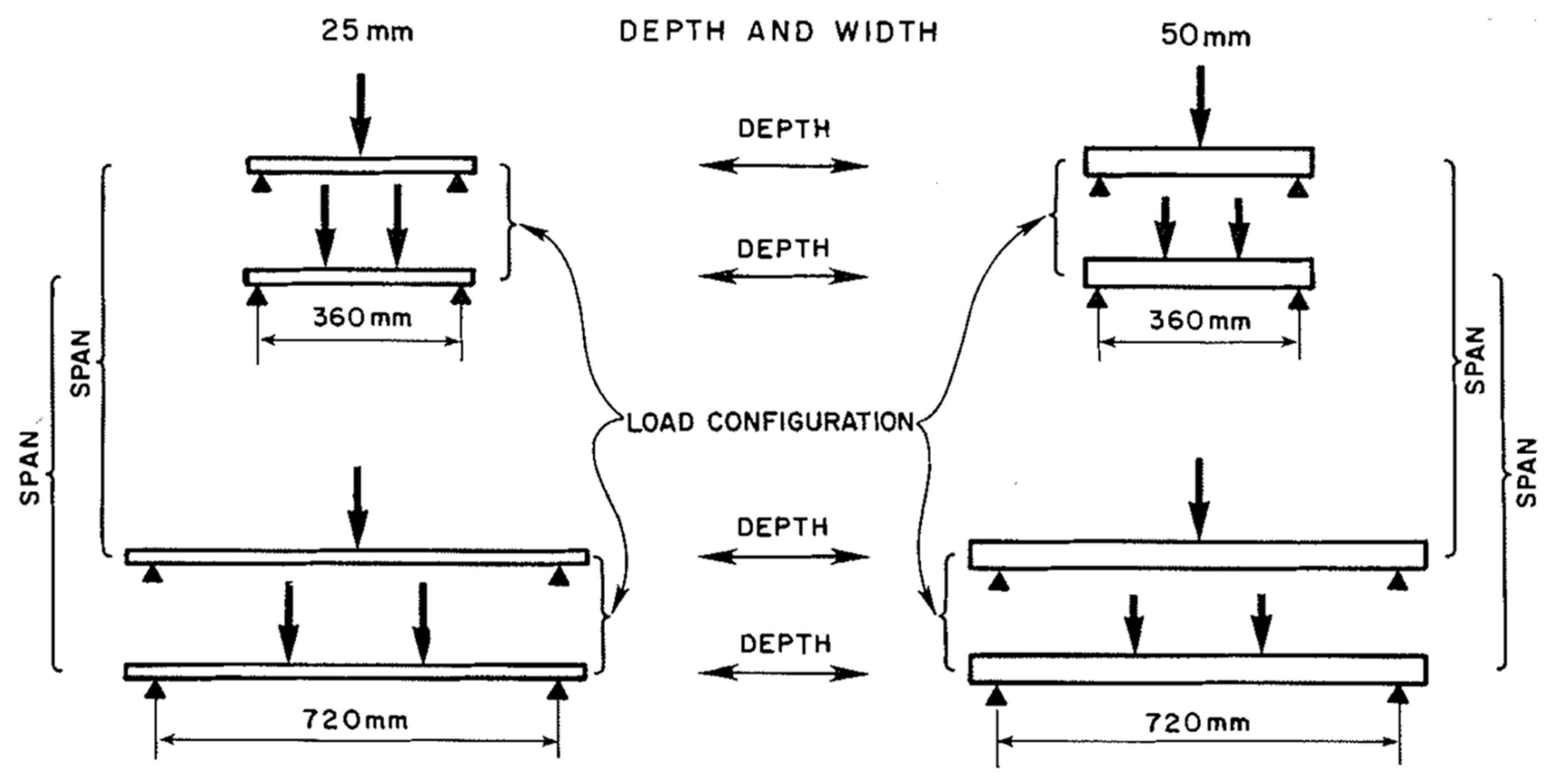
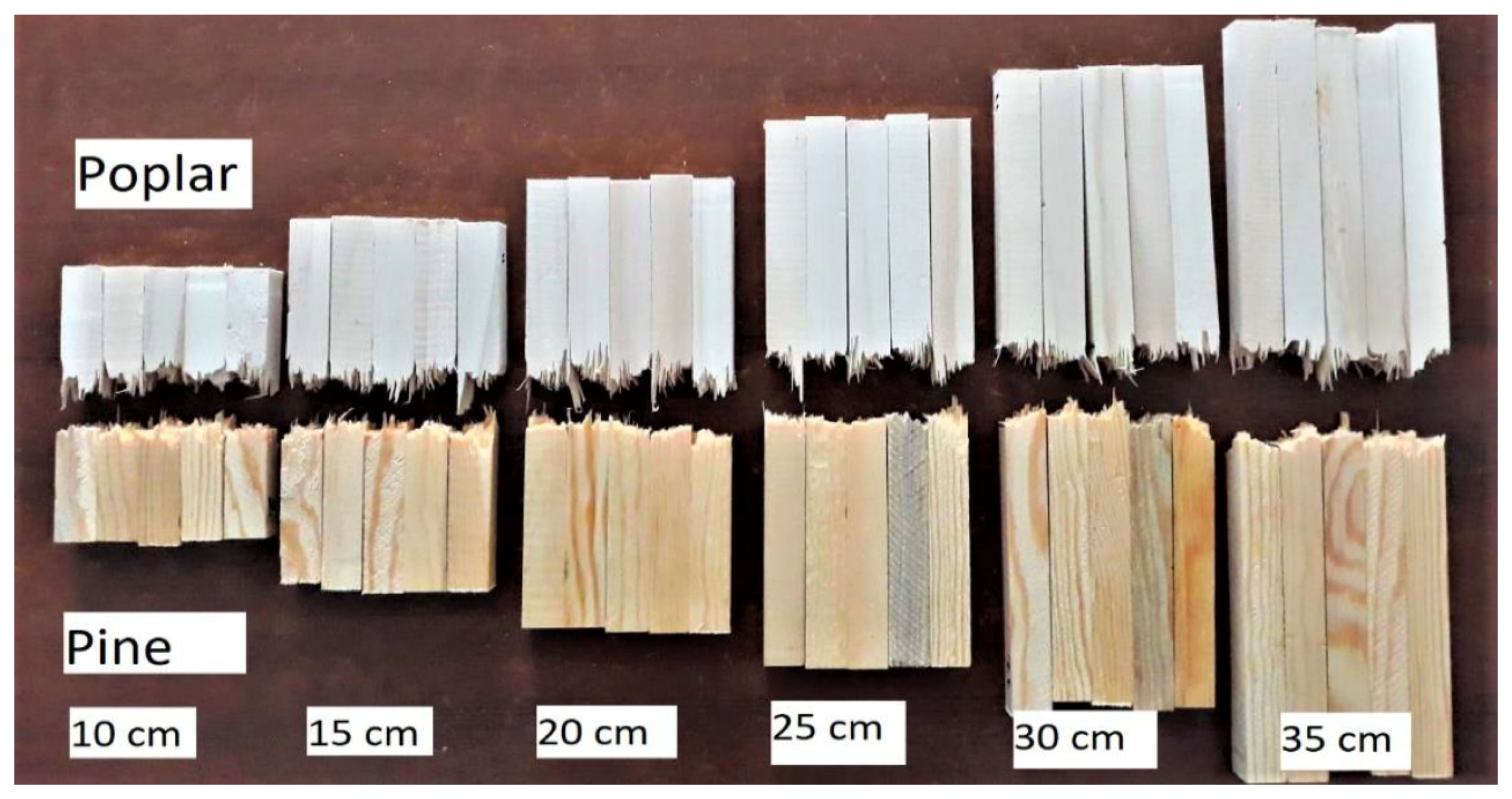
- Bal, B.C. Effect of span length on the impact bending strength of Poplar and Pine woods. BioResources 2021, 16, 4021–4026. [Google Scholar] [CrossRef]
- Xavier, J.; de Jesus, A.M.P.; Morais, J.J.L.; Pinto, J.M.T. Stereovision measurements on evaluating the modulus of elasticity of wood by compression tests parallel to the grain. Constr. Build. Mater. 2012, 26, 207–215. [Google Scholar] [CrossRef]
- Büyüksari, U.; As, N.; Dündar, T.; Sayan, E. Comparison of micro- and standard-size specimens in evaluating the flexural properties of Scots Pine wood. BioResources 2016, 11, 10540–10548. [Google Scholar] [CrossRef] [Green Version]
- Burawska-Kupniewska, I.; Mankowski, P.; Krzosek, S. Mechanical properties of machine stress graded sawn timber depending on the log type. Forests 2021, 12, 532. [Google Scholar] [CrossRef]
- Cao, Y.W.; Street, J.; Li, M.H.; Lim, H. Evaluation of the effect of knots on rolling shear strength of cross laminated timber (CLT). Constr. Build. Mater. 2019, 222, 579–587. [Google Scholar] [CrossRef]
- D’Amico, B.; Pomponi, F.; Hart, J. Global potential for material substitution in building construction: The case of cross laminated timber. J. Clean. Prod. 2021, 279, 123487. [Google Scholar] [CrossRef]
- Zhang, H.; Li, H.T.; Hong, C.K.; Xiong, Z.H.; Lorenzo, R.; Corbi, I.; Corbi, O. Size effect on the compressive strength of laminated bamboo lumber. ASCE J. Mater. Civ. Eng. 2021, 33, 04021161. [Google Scholar] [CrossRef]
- Fratzl, P.; Burgert, I.; Keckes, J. Mechanical model for the deformation of the wood cell wall. Z. Met. 2004, 95, 579–584. [Google Scholar] [CrossRef]
- Mishnaevsky, L.; Qing, H. Micromechanical modelling of mechanical behaviour and strength of wood: State-of-the-art review. Comput. Mater. Sci. 2008, 44, 363–370. [Google Scholar] [CrossRef]
- Guindos, P.; Guaita, M. A three-dimensional wood material model to simulate the behavior of wood with any type of knot at the macro-scale. Wood Sci. Technol. 2013, 47, 585–599. [Google Scholar] [CrossRef]
- Malek, S.; Gibson, L.J. Multi-scale modelling of elastic properties of balsa. Int. J. Solids Struct. 2017, 113, 118–131. [Google Scholar] [CrossRef]
- Koman, S.; Feher, S.; Abraham, J.; Taschner, R. Effect of knots on the bending strength and the modulus of elasticity of wood. Wood Res. 2013, 58, 617–626. [Google Scholar]
- Guindos, P.; Guaita, M. The analytical influence of all types of knots on bending. Wood Sci. Technol. 2014, 48, 533–552. [Google Scholar] [CrossRef]
- Wheel, M.A.; Frame, J.C.; Riches, P.E. Is smaller always stiffer? On size effects in supposedly generalised continua. Int. J. Solids Struct. 2015, 67, 84–92. [Google Scholar] [CrossRef] [Green Version]
- Anderson, W.B.; Lakes, R.S. Size effects due to Cosserat elasticity and surface damage in closed-cell polymethacrylimide foam. J. Mater. Sci. 1994, 29, 6413–6419. [Google Scholar] [CrossRef]


| Length. | Pillars with Both Ends Rounded. | Pillars with One End Flat, and the Other Rounded. | Pillars with Both Ends Flat. | ||||
|---|---|---|---|---|---|---|---|
| Diameter. | Breaking Weight. | Diameter. | Breaking Weight. | Diameter. | Breaking Weight. | ||
| Wrought iron. | inches. | inch. | lbs. | inch. | lbs. | inch. | lbs. |
| 1·017 | 1808 | 1·02 | 3355 | 1·02 | 5280 | ||
| 1·015 | 3938 | 1·03 | 8137 | 1·02 | 12,990 | ||
| 1·015 | 15,480 | 1·015 | 21,335 | 1·015 | 23,371 | ||
| 1·015 | 15,480 | 1·015 | 21,187 disc. | 1·015 | 25,387 disc. | ||
| 1·005 | 23,535 | 1·015 | 26,227 | 1·005 | 27,099 | ||
| Steel. | 29·95 | ·87 | 10,516 | ·87 | 20,135 | ·87 | 26,059 |
| Timber. | Side of square. 1·75 | 3197 | Side of square. 1·75 | 6109 | Side of square. 1·75 | 9625 | |
| Specimen Label | Dimensions | ||
|---|---|---|---|
| Cross-Sectional Area/mm2 | |||
| Width/mm | Length/mm | Height/mm | |
| 1 | 10 | 10 | 10 |
| 2 | 10 | 10 | 20 |
| 3 | 10 | 10 | 30 |
| 4 | 20 | 20 | 30 |
| 5 | 30 | 30 | 30 |
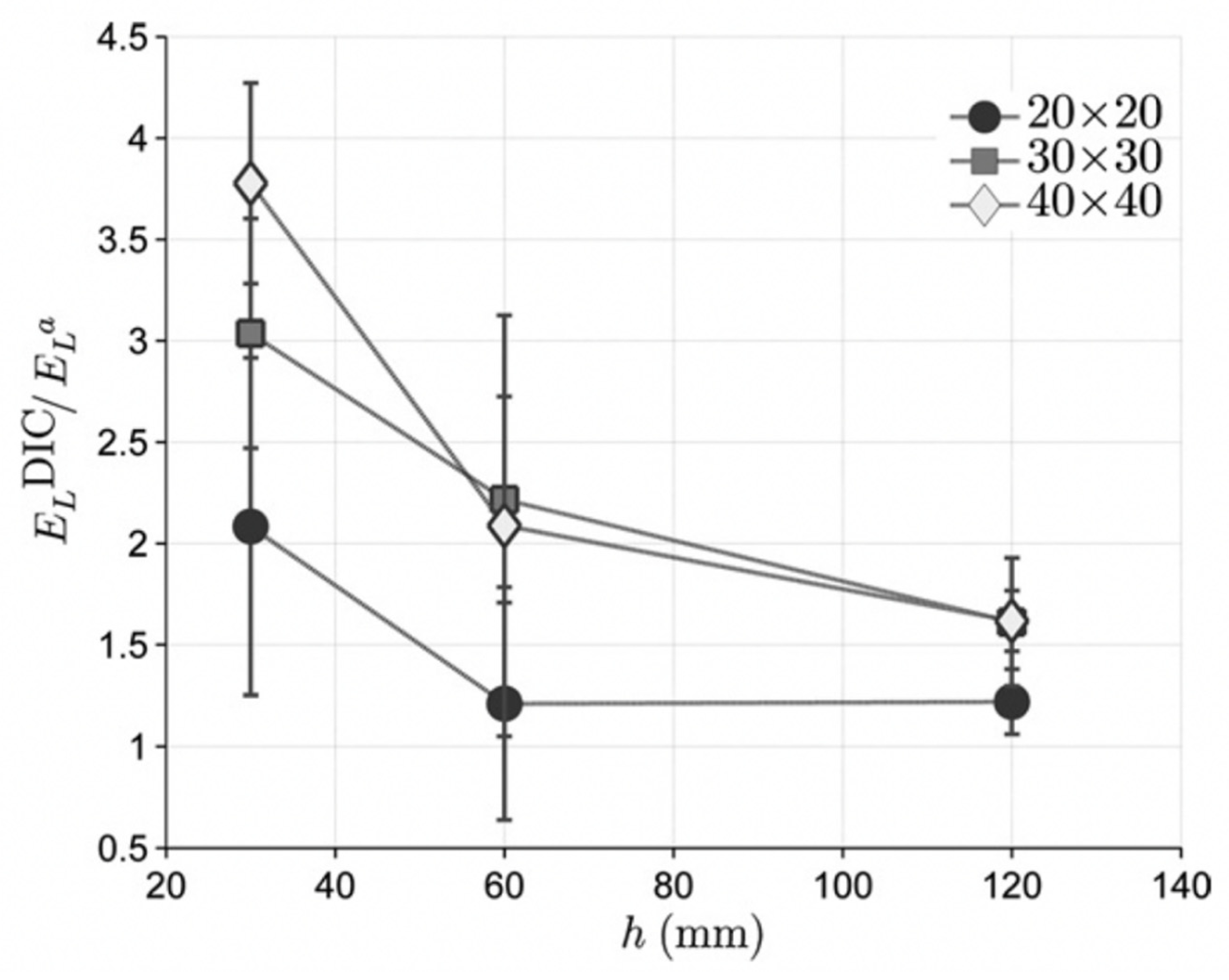
| Cross-Section/mm2 | Height/mm | ||
|---|---|---|---|
| 30 | 60 | 120 | |
| 20 | 15.7 ± 2.7 GPa | 15.9 ± 3.1 GPa | 14.5 ± 2.0 GPa |
| 30 | 16.9 ± 2.9 GPa | 15.1 ± 3.0 GPa | 15.1 ± 2.9 GPa |
| 40 | 18.1 ± 1.7 GPa | 16.1 ± 2.7 GPa | 15.8 ± 2.3 GPa |
Publisher’s Note: MDPI stays neutral with regard to jurisdictional claims in published maps and institutional affiliations. |
© 2022 by the authors. Licensee MDPI, Basel, Switzerland. This article is an open access article distributed under the terms and conditions of the Creative Commons Attribution (CC BY) license (https://creativecommons.org/licenses/by/4.0/).
Share and Cite
Walley, S.M.; Rogers, S.J. Is Wood a Material? Taking the Size Effect Seriously. Materials 2022, 15, 5403. https://doi.org/10.3390/ma15155403
Walley SM, Rogers SJ. Is Wood a Material? Taking the Size Effect Seriously. Materials. 2022; 15(15):5403. https://doi.org/10.3390/ma15155403
Chicago/Turabian StyleWalley, Stephen M., and Samuel J. Rogers. 2022. "Is Wood a Material? Taking the Size Effect Seriously" Materials 15, no. 15: 5403. https://doi.org/10.3390/ma15155403
APA StyleWalley, S. M., & Rogers, S. J. (2022). Is Wood a Material? Taking the Size Effect Seriously. Materials, 15(15), 5403. https://doi.org/10.3390/ma15155403