
Evaluate Pavement Skid Resistance Performance Based on Bayesian-LightGBM Using 3D Surface Macrotexture Data


Abstract
:1. Introduction
- (1)
- In this paper, 200 sets of surface texture and friction data of different gradation types are collected. Meanwhile, 10 macro-texture parameters are extracted from the 3D texture data.
- (2)
- To overcome the drawbacks of poor nonlinear fitting performance and the limited accuracy of traditional methods, a LightGBM-based model for correlation analysis between 3D texture features and skid resistance is constructed, and the importance of 3D texture features is obtained.
- (3)
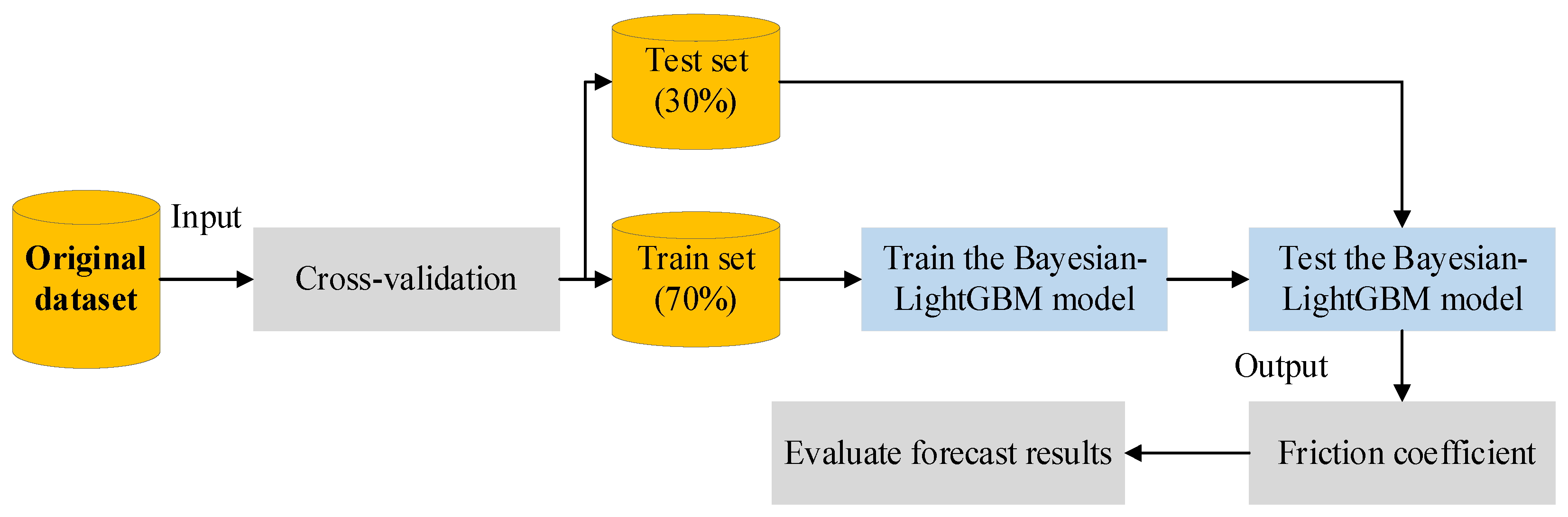
- A friction coefficient prediction model based on Bayesian-LightGBM is constructed according to the macro-texture features. A Bayesian optimization algorithm is used to improve the predictive performance of the model. The research method proposed in this paper effectively improves the evaluation accuracy of skid resistance performance based on 3D texture feature parameters. It is expected to promote the improvement of road intelligent detection technology.
2. Data and Method
2.1. Preparation of Asphalt Mixture Specimen
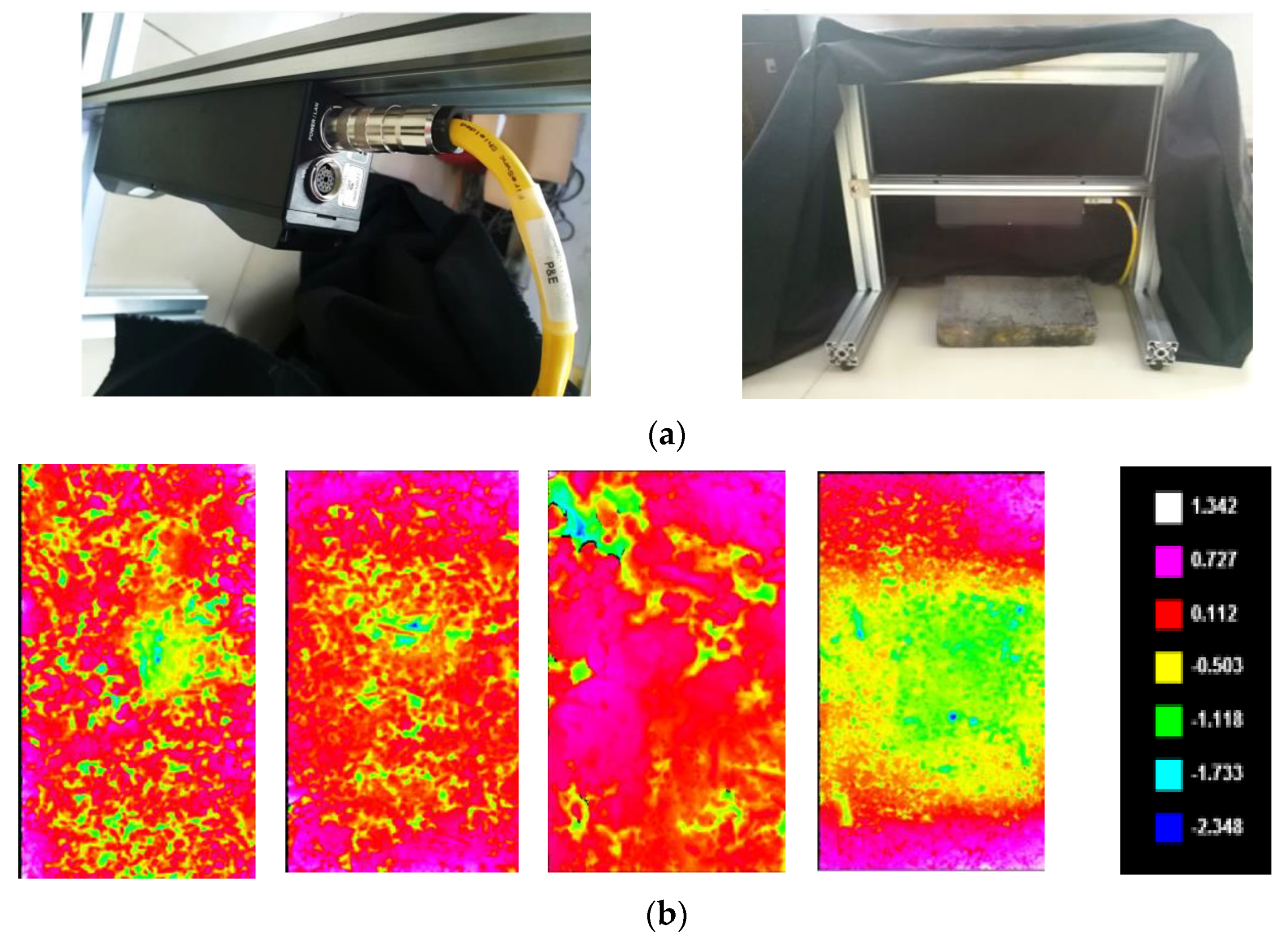
2.2. Collection of 3D Texture Data
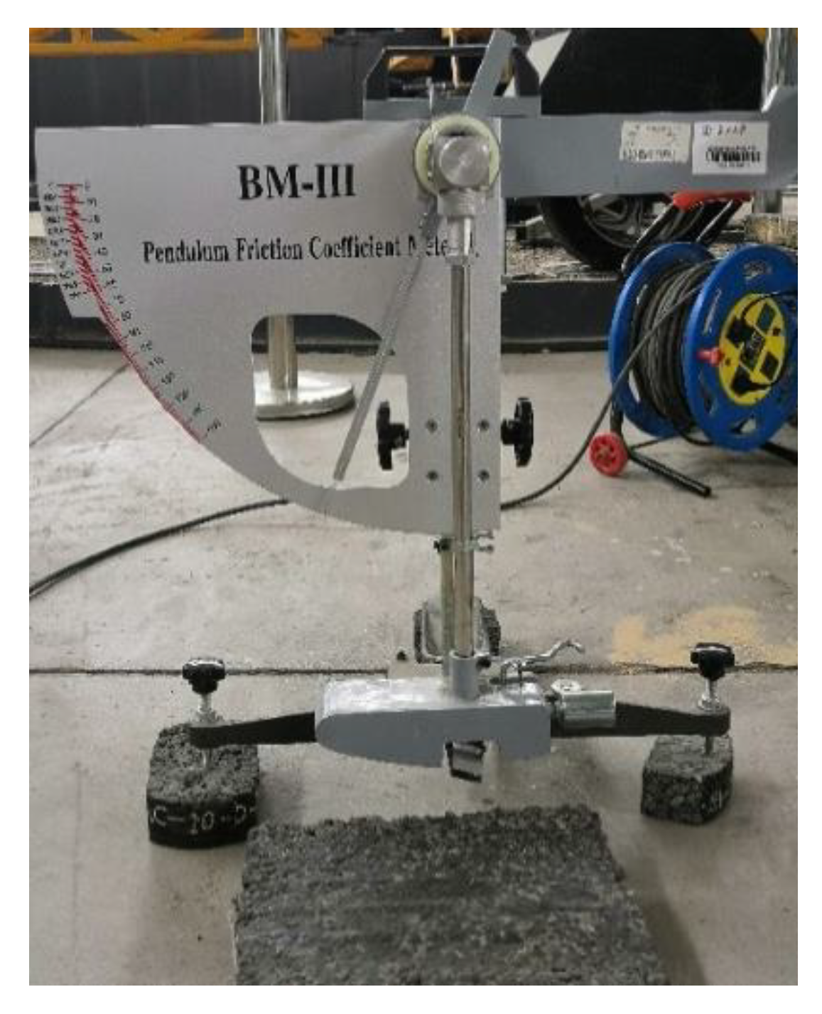
2.3. Skid Resistance Test
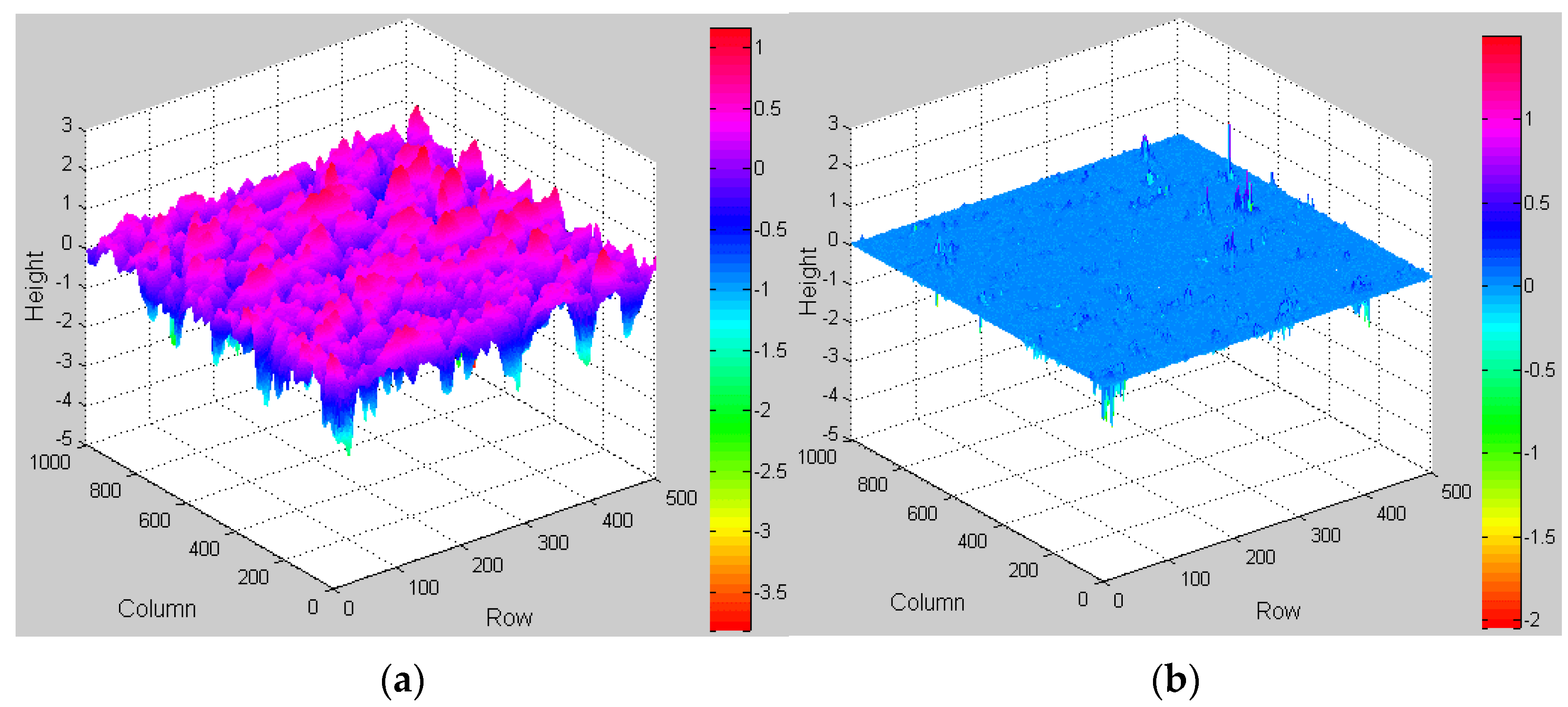
2.4. Preprocessing 3D texture Data
2.4.1. Repair of Missing Values in 3D Texture Point Cloud Data
2.4.2. Feature Extraction of 3D Macrotexture
- Correlated characterization indexes of height
- 2
- Correlated characterization indexes of wavelength
- 3
- Correlated characterization indexes of shape
3. Model Construction Method
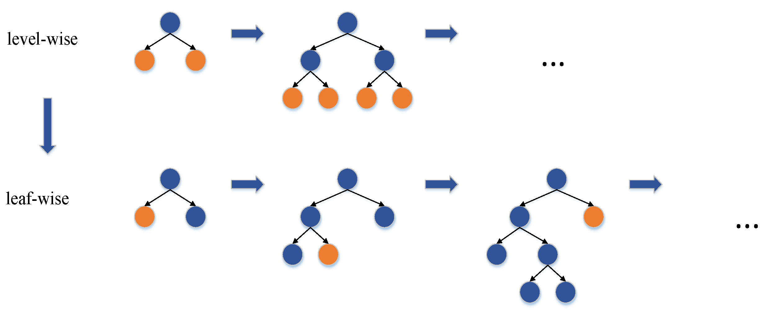
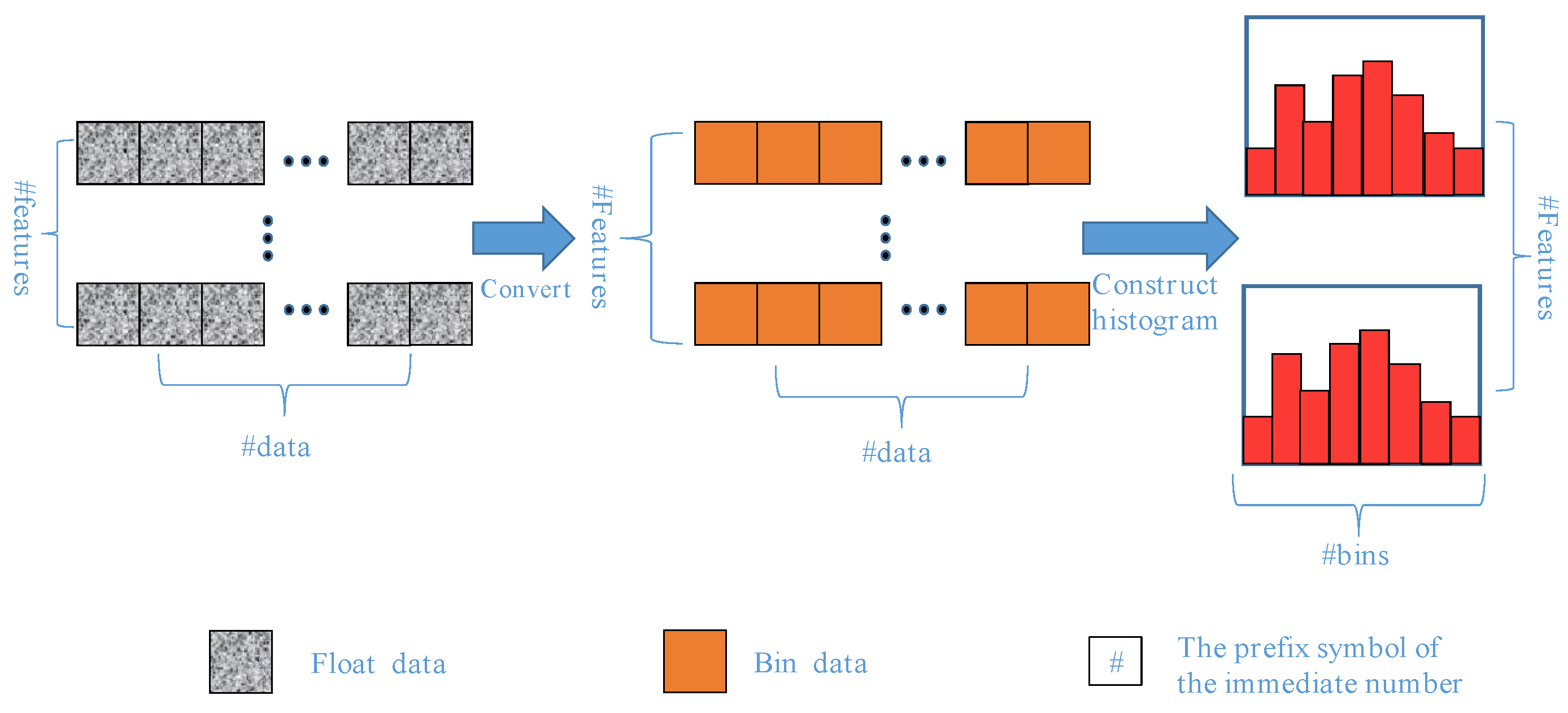
3.1. Light Gradient Boosting Machine
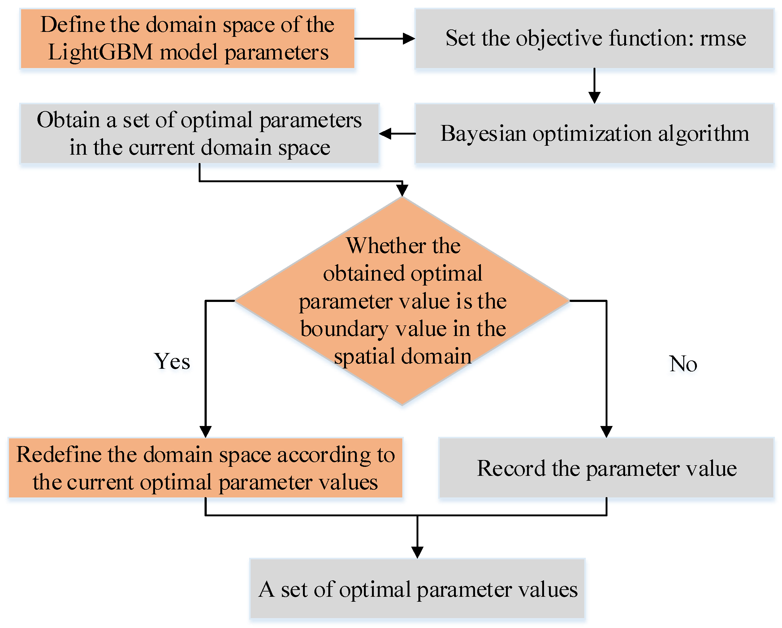
3.2. Bayesian-LightGBM Fusion Model Construction
3.3. Model Evaluation
4. Feature Selection and Friction Coefficient Prediction Results
4.1. Feature Selection Based on LightGBM
4.2. Prediction Results of Friction Coefficient Based on Bayesian-LightGBM Model
5. Results Discussion
5.1. Friction Coefficient and 3D Texture Features
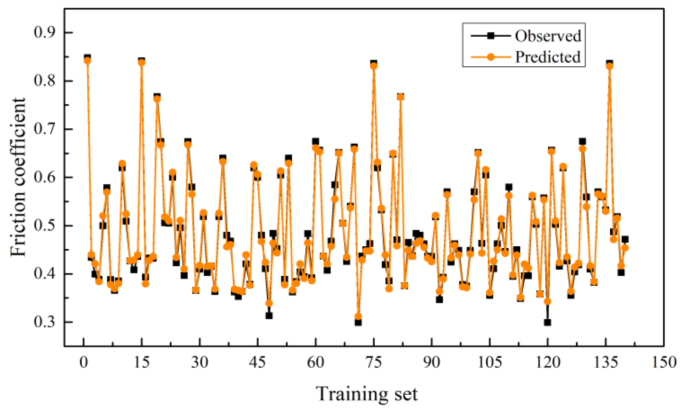
5.2. Analysis of the Predicted Friction Coefficient Results Based on Bayesian-LightGBM
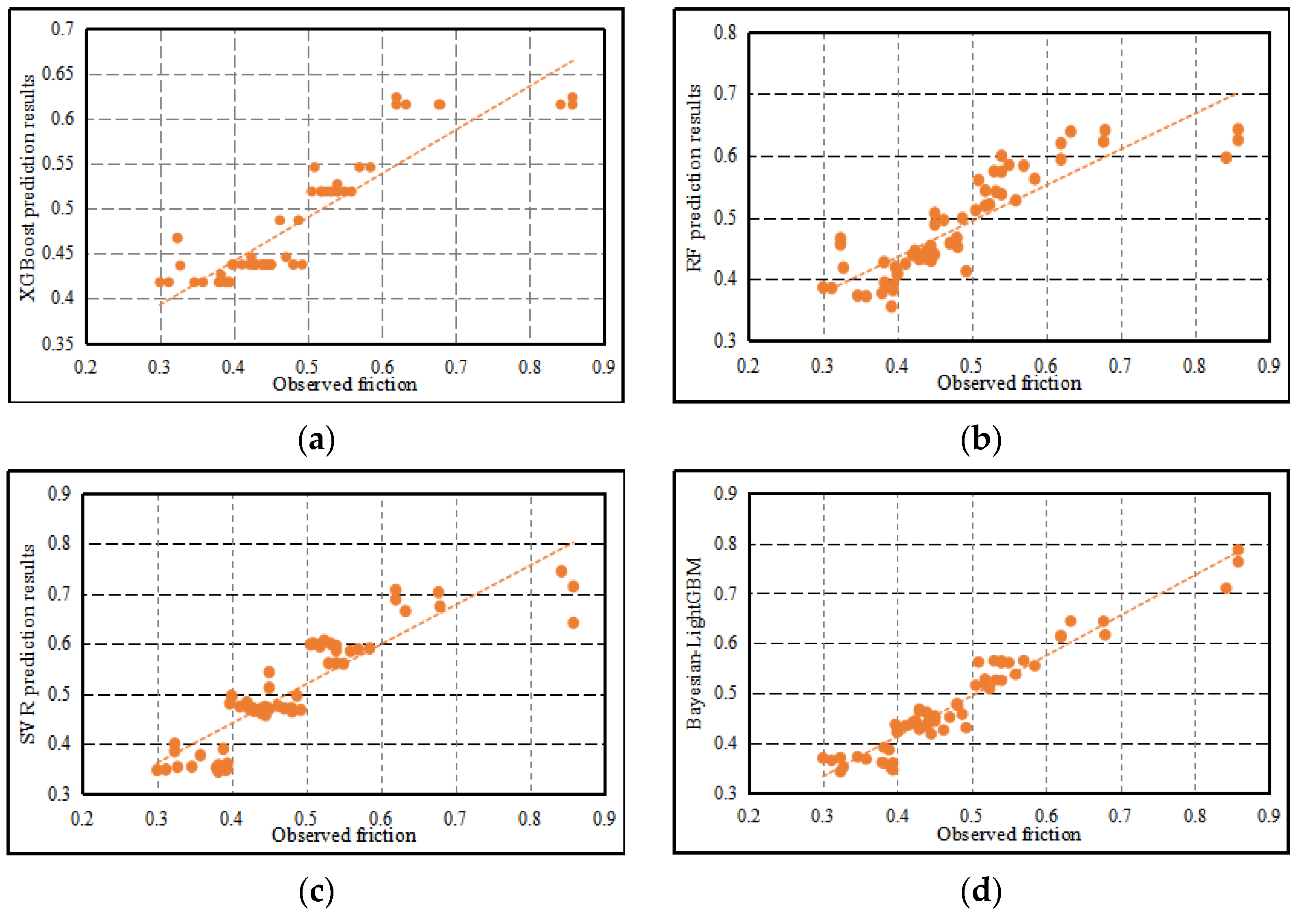
5.3. Comparison Analysis of Friction Coefficient Prediction Models
6. Conclusions and Future Research
- (1)
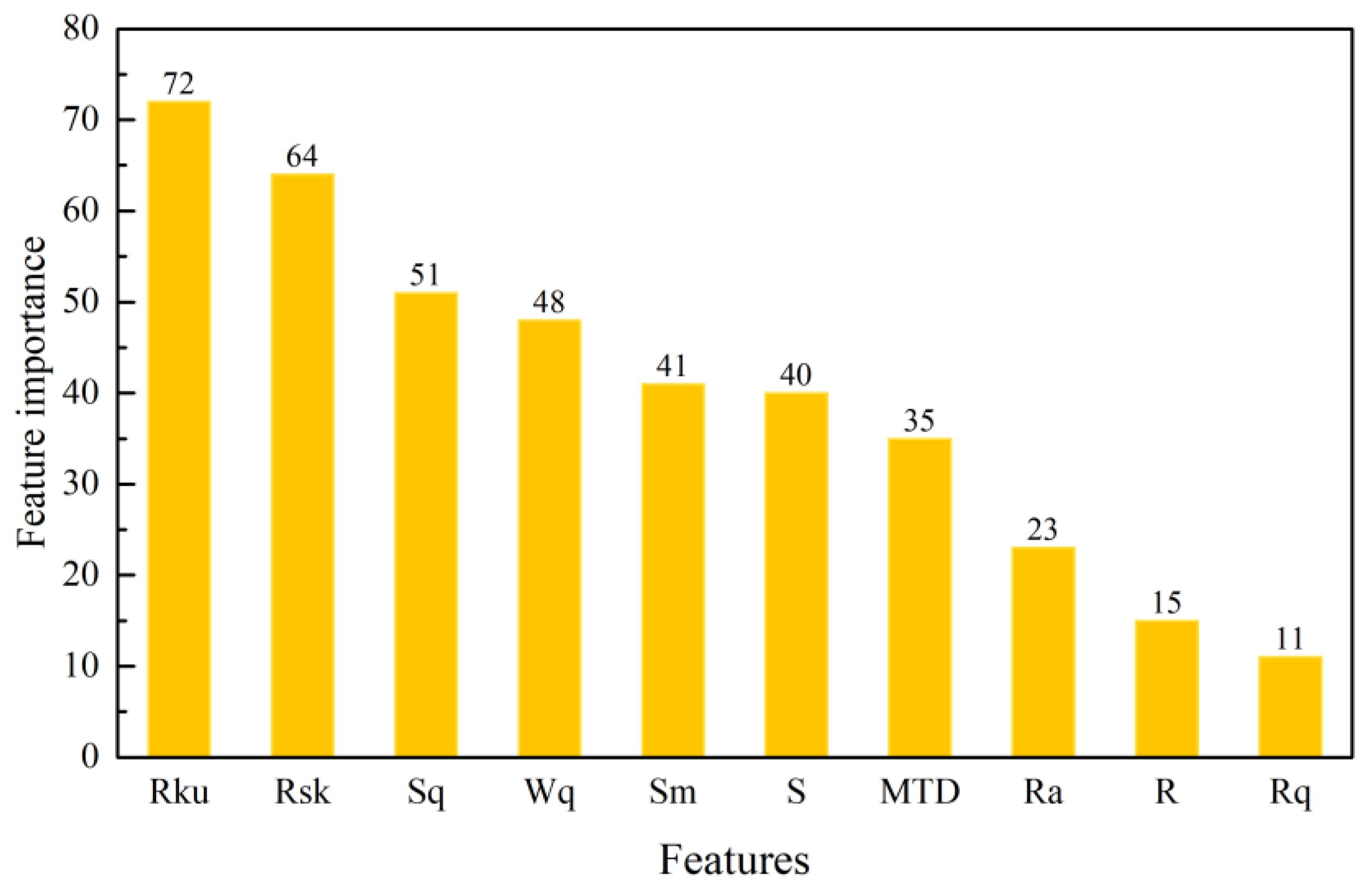
- The nonlinear relationship between 3D macrotexture features and skid resistance is analyzed based on LightGBM. The results of feature importance analysis show that each 3D macrotexture feature has a different degree of influence on the skid resistance performance. The 3D feature parameters , , and have a more significant effect on skid resistance performance, followed by , , , , and . and have lower feature importance scores, indicating that these features have the weakest correlation with the friction coefficient.
- (2)
- From the results of the feature importance analysis, we can conclude that the change of the pavement skid resistance performance results from the combined effect of different texture characteristic factors. A single index cannot reflect the influence mechanism of texture characteristics on skid resistance performance. More feature parameters should be selected to describe texture information, not limited to standard MTD features.
- (3)
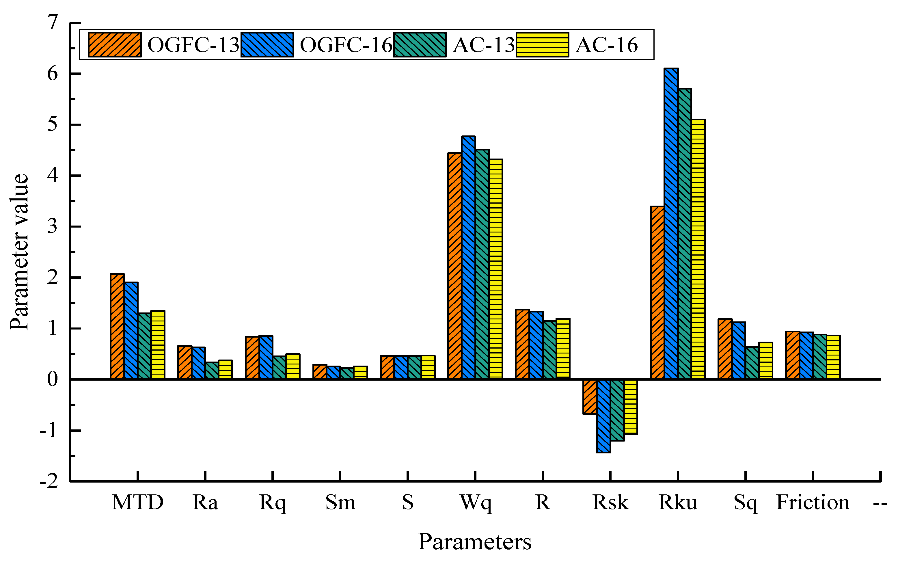
- The texture features and friction data of asphalt mixture specimens of different gradation types are analyzed. It is found that the specimens with OGFC-13 gradation type have the best skid resistance, followed by OGFC-16, AC-13, and AC-16. Compared with AC mixture specimen, the texture surface of OGFC mixture specimen has more obvious height characteristics and higher roughness. Therefore, the skid resistance of OGFC mixture specimens is better than that of AC.
- (4)
- Bayesian-LightGBM is more suitable than traditional model to evaluate the effect of surface texture on skid resistance performance. By discussing the performance of the proposed model on the training set and test set, it is proved that the model has strong generalization ability and can effectively adapt to the data set with the same distribution as the original data.
- (5)
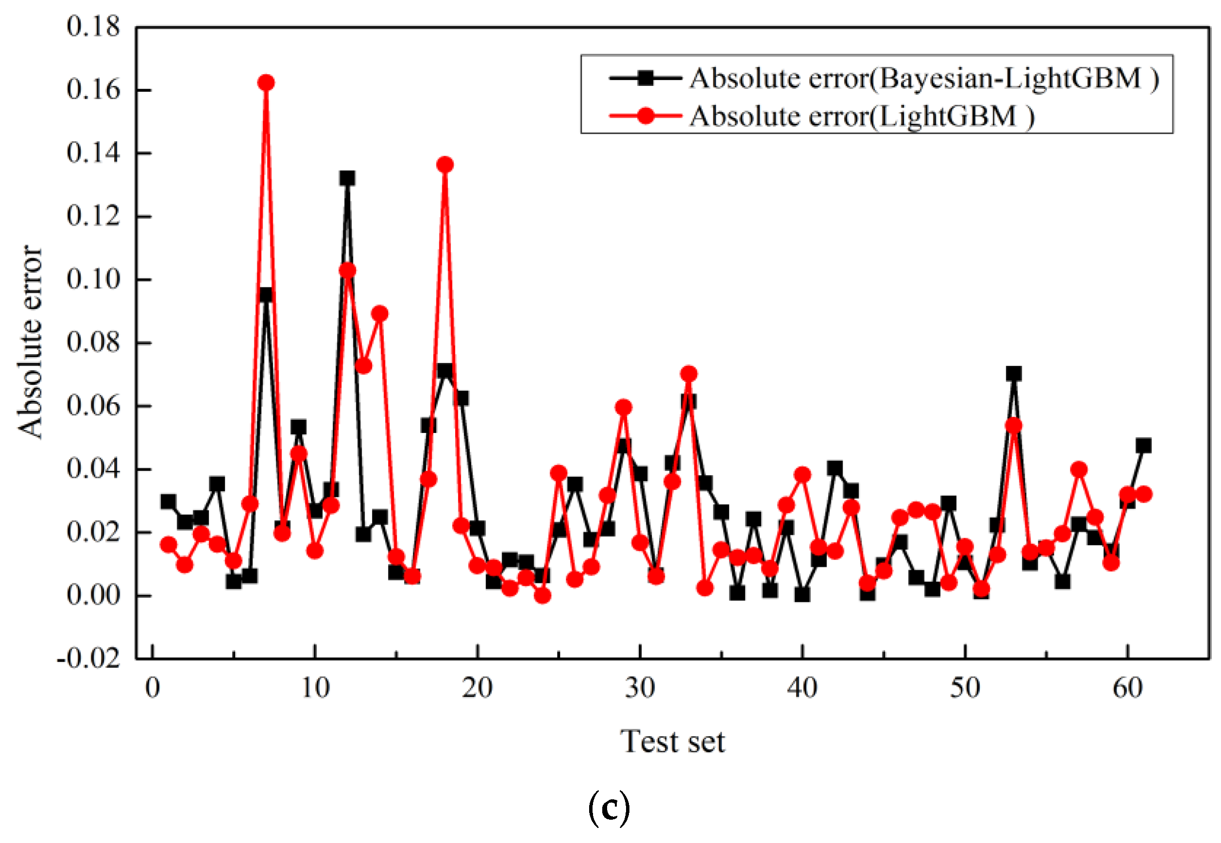
- Compared with RF, XGBoost, SVR, and LightGBM, the of the proposed Bayesian-LightGBM model is increased by 18%, 13%, 13.4%, and 3%, respectively. The comparison results show that the Bayesian-LightGBM model can accurately fit the friction coefficient by using 3D macrotexture features. Bayesian optimization algorithm improves the nonlinear fitting ability of the LightGBM model under multi-dimensional condition.
Author Contributions
Funding
Institutional Review Board Statement
Informed Consent Statement
Data Availability Statement
Conflicts of Interest
References
- Yu, J.; Zhang, B.; Long, P.; Chen, B.; Guo, F. Optimizing the texturing parameters of concrete pavement by balancing skid-resistance performance and driving stability. Materials 2021, 14, 6137. [Google Scholar] [CrossRef] [PubMed]
- Guo, F.; Pei, J.; Zhang, J.; Li, R.; Zhou, B.; Chen, Z. Study on the skid resistance of asphalt pavement: A state-of-the-art review and future prospective. Constr. Build. Mater. 2021, 303, 124411. [Google Scholar] [CrossRef]
- Yu, M.; You, Z.; Wu, G.; Kong, L.; Liu, C.; Gao, J. Measurement and modeling of skid resistance of asphalt pavement: A review. Constr. Build. Mater. 2020, 260, 119878. [Google Scholar] [CrossRef]
- Pomoni, M.; Plati, C.; Loizos, A.; Yannis, G. Investigation of pavement skid resistance and macrotexture on a long-term basis. Int. J. Pavement Eng. 2022, 23, 1060–1069. [Google Scholar] [CrossRef]
- Kane, M. A Contribution of the Analysis of the Road Macrotexture and Microtexture Roles vis-à-vis Skid Resistance. J. Test. Eval. 2021, 50, 744–754. [Google Scholar] [CrossRef]
- Wang, T.; Hu, L.; Pan, X.; Xu, S.; Yun, D. Effect of the compactness on the texture and friction of asphalt concrete intended for wearing course of the road pavement. Coatings 2020, 10, 192. [Google Scholar] [CrossRef] [Green Version]
- Yan, B.; Mao, H.; Zhong, S.; Zhang, P. Experimental study on wet skid resistance of asphalt pavements in icy conditions. Materials 2019, 12, 1201. [Google Scholar] [CrossRef] [Green Version]
- Liang, J.; Gu, X.; Chen, Y.; Ni, F.; Zhang, T. A novel pavement mean texture depth evaluation strategy based on three-dimensional pavement data filtered by a new filtering approach. Measurement 2020, 166, 108265. [Google Scholar] [CrossRef]
- Dan, H.; Gao, L.; Wang, H.; Tang, J. Discrete-Element Modeling of Mean Texture Depth and Wearing Behavior of Asphalt Mixture. J. Mater. Civ. Eng. 2022, 34, 04022027. [Google Scholar] [CrossRef]
- Huyan, J.; Li, W.; Tighe, S.; Sun, Z.; Sun, H. Quantitative analysis of macrotexture of asphalt concrete pavement surface based on 3D data. Transp. Res. Rec. 2020, 2674, 732–744. [Google Scholar] [CrossRef]
- Wang, Y.; Yang, Z.; Liu, Y.; Sun, L. The characterisation of three-dimensional texture morphology of pavement for describing pavement sliding resistance. Road Mater. Pavement Des. 2019, 20, 1076–1095. [Google Scholar] [CrossRef]
- Pranjić, I.; Deluka-Tibljaš, A. Pavement Texture–Friction Relationship Establishment via Image Analysis Methods. Materials 2022, 15, 846. [Google Scholar] [CrossRef]
- Song, W.M. Correlation between morphology parameters and skid resistance of asphalt pavement. Transp. Saf. Environ. 2022, 4, tdac002. [Google Scholar] [CrossRef]
- Du, Y.; Qin, B.; Weng, Z.; Wu, D.; Liu, C. Promoting the pavement skid resistance estimation by extracting tire-contacted texture based on 3D surface data. Constr. Build. Mater. 2021, 307, 124729. [Google Scholar] [CrossRef]
- Ji, J.; Jiang, T.; Ren, W.; Dong, Y.; Hou, Y.; Li, H. Precise Characterization of Macro-texture and Its Correlation with Anti-skidding Performance of Pavement. J. Test. Eval. 2022, 50. [Google Scholar] [CrossRef]
- Han, S.; Liu, M.; Fwa, T.F. Testing for low-speed skid resistance of road pavements. Road Mater. Pavement Des. 2020, 21, 1312–1325. [Google Scholar] [CrossRef]
- Wang, Y.; Lai, X.; Zhou, F.; Xue, J. Evaluation of pavement skid resistance using surface three-dimensional texture data. Coatings 2020, 10, 162. [Google Scholar] [CrossRef] [Green Version]
- Kováč, M.; Brna, M.; Decký, M. Pavement Friction Prediction Using 3D Texture Parameters. Coatings 2021, 11, 1180. [Google Scholar] [CrossRef]
- Hu, L.; Yun, D.; Liu, Z.; Du, S.; Zhang, Z.; Bao, Y. Effect of three-dimensional macrotexture characteristics on dynamic frictional coefficient of asphalt pavement surface. Constr. Build. Mater. 2016, 126, 720–729. [Google Scholar] [CrossRef]
- Al-Assi, M.; Kassem, E.; Nielsen, R. Using Close-Range Photogrammetry to Measure Pavement Texture Characteristics and Predict Pavement Friction. Transp. Res. Rec. 2020, 2674, 794–805. [Google Scholar] [CrossRef]
- Yang, G.; Wang, K.C.P.; Li, J.Q. Multiresolution analysis of three-dimensional (3D) surface texture for asphalt pavement friction estimation. Int. J. Pavement Eng. 2021, 22, 1882–1891. [Google Scholar] [CrossRef]
- Athiappan, K.; Kandasamy, A.; Mohamed, M.J.S.; Parthiban, P.; Balasubramanian, S. Prediction modeling of skid resistance and texture depth on flexible pavement for urban roads. Mater. Today: Proc. 2022, 52, 923–929. [Google Scholar] [CrossRef]
- Pattanaik, M.L.; Choudhary, R.; Kumar, B. Prediction of frictional characteristics of bituminous mixes using group method of data handling and multigene symbolic genetic programming. Eng. Comput. 2020, 36, 1875–1888. [Google Scholar] [CrossRef]
- Pérez-Acebo, H.; Gonzalo-Orden, H.; Findley, D.J.; Rojí, E. A skid resistance prediction model for an entire road network. Constr. Build. Mater. 2020, 262, 120041. [Google Scholar] [CrossRef]
- Galvis Arce, O.D.; Zhang, Z. Skid resistance deterioration model at the network level using Markov chains. Int. J. Pavement Eng. 2021, 22, 118–126. [Google Scholar] [CrossRef]
- Deng, Q.; Zhan, Y.; Liu, C.; Qiu, Y.; Zhang, A. Multiscale power spectrum analysis of 3D surface texture for prediction of asphalt pavement friction. Constr. Build. Mater. 2021, 293, 123506. [Google Scholar] [CrossRef]
- Goulias, D.G.; Awoke, G.S. Novel approach to pavement friction analysis with advanced statistical methods using structural equation modelling. Int. J. Pavement Eng. 2020, 21, 236–245. [Google Scholar] [CrossRef]
- Chen, D.; Han, S.; Ye, A.; Ren, X.; Wang, W.; Wang, T. Prediction of tire–pavement friction based on asphalt mixture surface texture level and its distributions. Road Mater. Pavement Des. 2020, 21, 1545–1564. [Google Scholar] [CrossRef]
- Huyan, J.; Li, W.; Tighe, S.; Zhang, Y.; Yue, B. Image-based coarse-aggregate angularity analysis and evaluation. J. Mater. Civ. Eng. 2020, 32, 04020140. [Google Scholar] [CrossRef]
- Li, S.; Zhao, X.; Zhou, G. Automatic pixel-level multiple damage detection of concrete structure using fully convolutional network. Comput. Aided Civ. Infrastruct. Eng. 2019, 34, 616–634. [Google Scholar] [CrossRef]
- Marcelino, P.; de Lurdes Antunes, M.; Fortunato, E.; Gomes, M.C. Machine learning approach for pavement performance prediction. Int. J. Pavement Eng. 2021, 22, 341–354. [Google Scholar] [CrossRef]
- Majidifard, H.; Jahangiri, B.; Buttlar, W.G.; Alavi, A.H. New machine learning-based prediction models for fracture energy of asphalt mixtures. Measurement 2019, 135, 438–451. [Google Scholar] [CrossRef]
- Pei, L.; Sun, Z.; Yu, T.; Li, W.; Hao, X.; Hu, Y.; Yang, C. Pavement aggregate shape classification based on extreme gradient boosting. Constr. Build. Mater. 2020, 256, 119356. [Google Scholar] [CrossRef]
- Najafi, S.; Flintsch, G.W.; Khaleghian, S.; Flintsch, G.W.; Khaleghian, S. Pavement friction management—Artificial neural network approach. Int. J. Pavement Eng. 2019, 20, 125–135. [Google Scholar] [CrossRef]
- Yu, M.; Xu, X.; Wu, C.; Li, S.; Chen, H. Research on the prediction model of the friction coefficient of asphalt pavement based on tire-pavement coupling. Adv. Mater. Sci. Eng. 2021, 2021, 1–10. [Google Scholar]
- Zhan, Y.; Li, J.Q.; Liu, C.; Wang, K.C.; Pittenger, D.M.; Musharraf, Z. Effect of aggregate properties on asphalt pavement friction based on random forest analysis. Constr. Build. Mater. 2021, 292, 123467. [Google Scholar] [CrossRef]
- Chen, N.; Xu, Z.; Liu, Z.; Chen, Y.; Miao, Y.; Li, Q.; Wang, L. Data Augmentation and Intelligent Recognition in Pavement Texture Using a Deep Learning. IEEE Trans. Intell. Transp. Syst. 2022, 1–10. [Google Scholar] [CrossRef]
- Qiu, Y.; Zhou, J.; Khandelwal, M.; Yang, H.; Yang, P.; Li, C. Performance evaluation of hybrid WOA-XGBoost, GWO-XGBoost and BO-XGBoost models to predict blast-induced ground vibration. Eng. Comput. 2021, 1–18. [Google Scholar] [CrossRef]
- Liang, J.; Bu, Y.; Tan, K.; Pan, J.; Yi, Z.; Kong, X.; Fan, Z. Estimation of Stellar Atmospheric Parameters with Light Gradient Boosting Machine Algorithm and Principal Component Analysis. Astron. J. 2022, 163, 153. [Google Scholar] [CrossRef]
- E303-93; Standard Test Method for Measuring Surface Frictional Properties Using the British Pendulum Tester. ASTM: West Conshohocken, PA, USA, 2018.
- ISO 16610-21:2011; Geometrical Product Specifications (GPS)—Filtration—Part 21: Linear Profile Filters: Gaussian Filters. ISO: Geneva, Switzerland, 2011.
- ISO 4287:1997; Geometrical Product Specifications (GPS)—Surface Texture: Profile Method—Terms, Definitions and Surface Texture Parameters. ISO: Geneva, Switzerland, 1997.
- Sun, Z.; Hao, X.; Li, W.; Huyan, J.; Sun, H. Asphalt pavement friction coefficient prediction method based on genetic-algorithm-improved neural network (GAI-NN) model. Can. J. Civ. Eng. 2022, 49, 109–120. [Google Scholar] [CrossRef]
- Rith, M.; Kim, Y.K.; Lee, S.W. Characterization of long-term skid resistance in exposed aggregate concrete pavement. Constr. Build. Mater. 2020, 256, 119423. [Google Scholar] [CrossRef]
- Hu, Y.J.; Sun, Z.Y.; Li, W.; Pei, L.L. Forecasting public bicycle rental demand using an optimized eXtreme Gradient Boosting model. J. Intell. Fuzzy Syst. 2022, 42, 1783–1801. [Google Scholar] [CrossRef]


| Asphalt Mixture | Mixture Gradation Type | Species | Number |
|---|---|---|---|
| Asphalt Concrete (AC) | AC-20 | 3 | 1 |
| AC-16 | 3 | 1 | |
| AC-13 | 3 | 1 | |
| AC-10 | 3 | 1 | |
| AC-5 | 3 | 1 | |
| Open Graded Friction Course (OGFC) | OGFC-16 | 3 | 1 |
| OGFC-13 | 3 | 1 | |
| OGFC-10 | 3 | 1 |
| Parameters | Parameter Meaning |
|---|---|
| Arithmetic mean deviation (mm) | Reflects the degree of dispersion of the profile amplitude relative to the baseline |
| Root mean square deviation (mm) | Reflects the standard deviation of the amplitude distribution of the random surface texture profile |
| Mean texture depth (mm) | Reflects the average depth of surface texture voids |
| Mean distance of profile unevenness (mm) | Reflects the intersection density of profile and centerline |
| Root mean square wavelength | Measures the average distance between the peaks (or valleys) of the texture profile in the sampling range |
| Surface roughness area ratio | Reflects the unevenness of the texture surface relative to the median surface |
| Mean distance between single profile peaks (mm) | Reflects the peak density of the profile |
| Skewness | Reflects the degree of asymmetry of the profile amplitude distribution deviating from the baseline |
| Steepness | Reflects the sharpness of the profile surface distribution |
| Root mean square slope | Reflects the root mean square of the slope of each point of the contour surface |
| Model Parameters | Parameter Adjustment Effect |
|---|---|
| max_depth | The maximum depth of the tree, when this value is large, the model is more complex and prone to overfitting |
| min_data_in_leaf | Minimum number of records for leaves, setting it to a larger value can prevent the tree from growing too deep |
| max_bin | Indicates the maximum number of features stored in the bin |
| num_leaves | It can be used to control the complexity of the tree |
| bagging_fraction | The proportion of data used in each iteration, used to speed up the training speed of the model |
| bagging_freq | Re-sampling is done every bagging_freq iterations, and the sampling ratio is bagging_fraction |
| feature_fraction | When the value is set to 0.8, it means that 80% of the features are randomly selected to construct a decision tree in each iteration |
| lambda_l1 | Regular term L1 |
| lambda_l2 | Regular term L2 |
| Evaluation Index | Equation | Explanation |
|---|---|---|
| is the observed value; is the predicted value; represents the mean of the set of data; m represents the sample size | ||
| RMSE | ||
| MAPE |
| Model Parameters | Optimal Parameter Value |
|---|---|
| max_depth | 20 |
| min_data_in_leaf | 1 |
| max_bin | 256 |
| num_leaves | 170 |
| bagging_fraction | 1 |
| bagging_freq | 73 |
| feature_fraction | 1 |
| lambda_l1 | 0.001 |
| lambda_l2 | 0.001 |
| Data Set | RMSE | MAPE | |
|---|---|---|---|
| Training set | 0.9800 | 0.0114 | 2.0325 |
| Test set | 0.9293 | 0.0356 | 5.5700 |
| Models | RMSE | MAPE | |
|---|---|---|---|
| RF | 0.7464 | 0.0616 | 7.496 |
| XGBoost | 0.7921 | 0.0691 | 8.534 |
| SVR | 0.7885 | 0.0604 | 9.183 |
| LightGBM | 0.8981 | 0.0412 | 5.8120 |
| Bayesian-LightGBM | 0.9293 | 0.0356 | 5.5700 |
Publisher’s Note: MDPI stays neutral with regard to jurisdictional claims in published maps and institutional affiliations. |
© 2022 by the authors. Licensee MDPI, Basel, Switzerland. This article is an open access article distributed under the terms and conditions of the Creative Commons Attribution (CC BY) license (https://creativecommons.org/licenses/by/4.0/).
Share and Cite
Hu, Y.; Sun, Z.; Han, Y.; Li, W.; Pei, L. Evaluate Pavement Skid Resistance Performance Based on Bayesian-LightGBM Using 3D Surface Macrotexture Data. Materials 2022, 15, 5275. https://doi.org/10.3390/ma15155275
Hu Y, Sun Z, Han Y, Li W, Pei L. Evaluate Pavement Skid Resistance Performance Based on Bayesian-LightGBM Using 3D Surface Macrotexture Data. Materials. 2022; 15(15):5275. https://doi.org/10.3390/ma15155275
Chicago/Turabian StyleHu, Yuanjiao, Zhaoyun Sun, Yuxi Han, Wei Li, and Lili Pei. 2022. "Evaluate Pavement Skid Resistance Performance Based on Bayesian-LightGBM Using 3D Surface Macrotexture Data" Materials 15, no. 15: 5275. https://doi.org/10.3390/ma15155275
APA StyleHu, Y., Sun, Z., Han, Y., Li, W., & Pei, L. (2022). Evaluate Pavement Skid Resistance Performance Based on Bayesian-LightGBM Using 3D Surface Macrotexture Data. Materials, 15(15), 5275. https://doi.org/10.3390/ma15155275