Article

Designing and Calculating the Nonlinear Elastic Characteristic of Longitudinal–Transverse Transducers of an Ultrasonic Medical Instrument Based on the Method of Successive Loadings

by
Huu-Dien Nguyen
1,2 and
Shyh-Chour Huang
1,*
1
Department of Mechanical Engineering, National Kaohsiung University of Science and Technology, No. 415, Jiangong Rd., Sanmin Dist, Kaohsiung City 807618, Taiwan
2
Institute of Engineering, HUTECH University, No. 475A, Dien Bien Phu Rd., Binh Thanh Dist, Ho Chi Minh City 700000, Vietnam
*
Author to whom correspondence should be addressed.
Materials 2022, 15(11), 4002; https://doi.org/10.3390/ma15114002
Submission received: 26 April 2022 / Revised: 27 May 2022 / Accepted: 2 June 2022 / Published: 4 June 2022
(This article belongs to the Special Issue Advanced Materials and Devices for Applied System Innovation)

Abstract

:
This paper presents a numerical method for studying the stress–strain state and obtaining the nonlinear elastic characteristics of longitudinal–transverse transducers. The authors propose a mathematical model that uses a direct numerical solution of the boundary value problem based on the plain curved rod equations in Matlab. The system’s stress–strain state and nonlinear elastic characteristic are obtained using the method of successive loadings based on the curved rod’s linearized equations. For most ultrasonic instruments, the operating frequency of ultrasonic vibrations is close to 20 kHz. On the other hand, the received own oscillation frequencies are close to the working range. Using the method of successive loadings in the mathematical complex Matlab, a numerical calculation of the stress–strain state of a flat, curved rod at large displacements has been carried out. The proposed model can be considered an initial approximation to the solution of the spatial problem of the longitudinal–torsional transducer.

1. Introduction

Since its inception, ultrasound-based diagnostic techniques have been increasingly widely used in medicine. Equipping ultrasound machines is the most basic investment in modern medical examination and treatment facilities. The larger the facility, the more advanced and expensive are its equipment. In addition to its diagnostic significance, ultrasound has low risks, wide application, and it is also the main source of income for conventional medical facilities. In the ultrasound machine, the transducer and its model (see Figure 1) are the parts that function the most, receiving and processing the initial signal. The probe set in this research is applied in the medical field. It mediates the analysis and transmission of data from the patient’s body contact and then outputs the data and encodes the image on the computer screen. Of course, in this research, only its mechanical behavior was studied [1,2,3,4,5].
This paper considers a geometrically nonlinear theory of rods. In this theory, the rod is modeled by a one-dimensional curve that has distributed inertial and stiffness characteristics. The deformations of bending, shear, and tension–compression are taken into account, and no restrictions are imposed on the values of displacements and turns. In the plane problem, each point of such a rod has three degrees of freedom—two translational and one rotational. This theory is called the Timoshenko Theory, often known as Geometrically Exact Theory [6,7,8,9,10].
Considering all rod stiffnesses (tension–compression, shear, and bending) is necessary when calculating highly loaded elements of structures, such as high-rise, multi-story buildings, offshore oil platforms, chimneys, and masts. The linear theory of perfectly elastic rods is usually used as a design model. However, geometric nonlinearity must be taken into account, considering that heavy loads lead to large changes in the rod’s geometry [11,12,13].
The general nonlinear formulation of the problems of the statics and stability of rods and their systems has not yet been widely implemented in software systems used in design practice. Further, the accounting for geometric nonlinearity in these complexes is based on a simplified formulation that only considers the effect of the compressive force on the bending stiffness of the rod (i.e., the so-called calculation according to the deformed scheme). Thus, constructing more complex nonlinear models will make it possible to obtain a more accurate solution in some cases [14].
Presently, the calculation of stability is carried out using approximate methods, which do not accurately assess the real stresses in structures. In addition, all computer programs used to calculate the stability of structures ignore the tensile-compressive stiffness and only take into account either the bending stiffness according to the Euler formula or the bending and shear stiffness according to the Engesser formula [15].
Understanding longitudinal vibrations of rods is a classical structural mechanics theme. The standard problem involving a rod with uniform cross-section excited by continuous or point-loads is described in several textbooks, such as in Clough and Penzien, and Rao. In these references the governing equation is shown to be a linear partial differential equation that is solved, for instance, by the method of separation of variables, or by the boundary element method. A relevant development of this problem relates to vibrations of rods with variable cross-sections. In this context, Eisenberger proposed a method for obtaining the exact longitudinal vibration frequencies of tapered rods. Specifically, he considered the case of rods with polynomial variations of the cross-sectional area. Other exact solutions were derived by Abrate who studied the vibration of conical rods, and by Bapat who considered exponential and catenoidal rods. Further, Kumar investigated the case of rods having polynomial, as well as sinusoidal variations of the cross-sectional area by representing the mode shapes in terms of Bessel, Neumann, and trigonometric functions. Nonlinear problems were considered by Wie and Gui-tong and Cveticanin and Uzelac. Specifically, Wei and Gui-tong applied an inverse scattering method for analyzing strain solitons in a rod with nonlinear elastic constitutive law [16,17,18,19].
Furthermore, considerable research is devoted to the field of rod stability and nonlinear deformation. Researchers were engaged in solving structural mechanics problems in a variational setting. Noteworthily, Eliseev VV also made a significant contribution to the development of the nonlinear theory of rods [20].

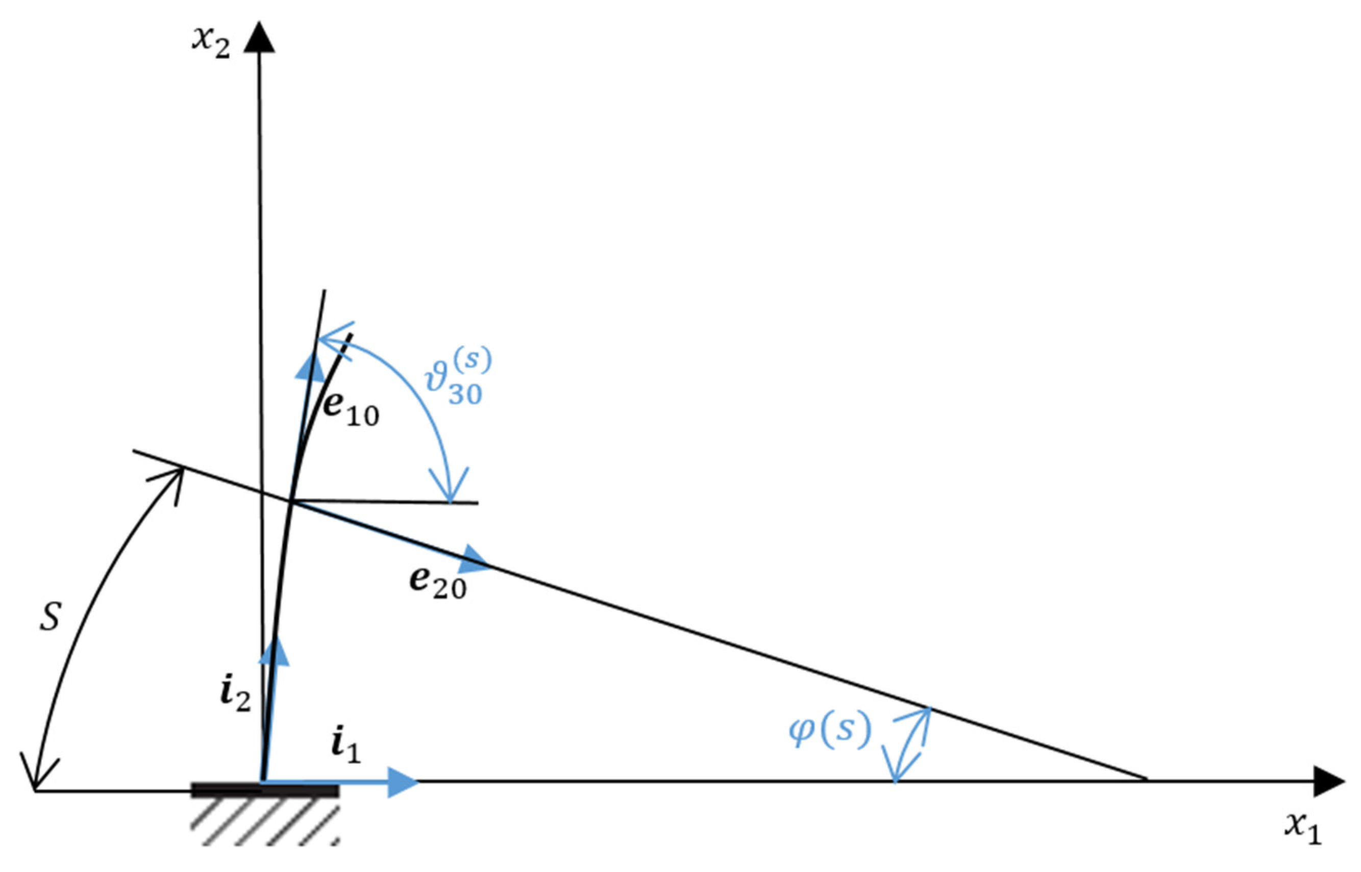
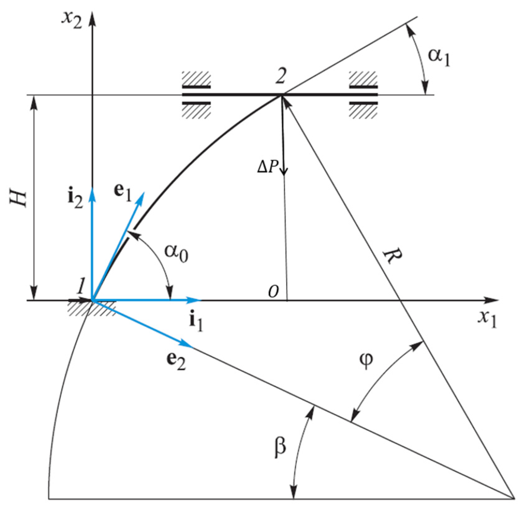
2. The Method of Successive Loadings (MSL)

When solving problems in loading structures comprising rod elements, one often has to deal with large displacements of these elements (i.e., commensurate with the length of the rod). Several methods for solving nonlinear problems applicable to the calculation of plates, shells, membranes, and rods have been developed in the mechanics of deformable solids. This section describes a relatively simple MSL to solve the plane problems of rods’ mechanics, which is accurate enough for everyday engineering practice. The results of numerical studies on rods exposed to different loads are presented, of which exact analytical solutions are available in the literature. In addition, the accuracy of the proposed method of solving such problems is demonstrated. The described method for numerically investigating flat rods’ deep deformation can be easily applied to studying constructions of spatial rods of arbitrarily complex geometry. This section may be of interest to specialists in the field of rod mechanics [21,22,23,24,25].
This variant of numerical solution for nonlinear equations leads to linear equations for each discrete increase in load. For the mth loading of the rod, the external force F(m) = kF, where m is the loading step number; k is a parameter that determines the part of the total load at each loading step, k = 1/m (m-the number of loading steps). Thus, the solution to the deformation of the rod at large displacements is replaced by a consistent solution of a number of problems on the deformation of the rod at small displacements (i.e., linear problems).
Before considering a flat rod, allow us to show how the system of MSL equations can be obtained using the example of a spatial rod. We will take, as a basis for further research, the nonlinear system of equilibrium equations spatially curved rod in connected axes [26,27,28,29,30]:
d Q d η + χ × Q + q + i = 1 n F ( 1 ) δ ( η η i ) = 0 ; d M d η + χ × M + e 1 × Q + μ + ν = 1 n T ( ν ) δ ( η η ν ) = 0 ; L 1 d θ d η + L 2 χ 0 ( 1 ) A 1 M = 0 ; d u d η + χ × u + ( l 11 1 ) e 1 + l 21 e 2 + l 31 e 3 = 0 ; M = A ( χ χ 0 ( 1 ) ) ,
where Q, M, u are vectors of internal forces, moments, and displacements of points of the centerline of the rod, respectively; η is a dimensionless arc coordinate, η = s / l (s is the dimensional coordinate; l is the rod length); χ and χ 0 ( 1 ) are vectors, whose components are the curvature of the rod’s centerline after loading living and in a natural state; q and μ are distributed forces and moments; F ( i ) and T ( ν ) are concentrated forces and moments; δ ( η η i ) , δ ( η η ν ) are generalized Dirac functions defined in the corresponding coordinates, η i , η ν ; θ is the vector of the angles of rotation of the connected axes relative to the position in the natural (unloaded) state; θ = ϑ i e i ( ϑ i refers to the components of the vector of rotation angles; e i is the unit vectors of the bound deformed main basis); A refers to the diagonal matrix dimensionless torsional stiffnesses; l i j are the elements of the transformation matrix of basis vectors, L. The matrices L 1 and L 2 are included in the system of Equation (1), as well as the matrix L.
We obtain the system of MSL equations to measure the first equation for internal forces.
At the first step of loading:
F = Δ F ( 1 )
here and below, the superscript corresponds to the loading step number. We will take all external forces,
F = q + i = 1 n F ( i ) δ ( η η i )
and all external moments,
T = q + ν = 1 k T ( ν ) δ ( η η i ) ,
Then,
d Δ Q ( 1 ) d η + ( χ 0 + Δ χ ( 1 ) ) Δ Q ( 1 ) + Δ F ( 1 ) = 0
where Δ Q ( 1 ) is the increment of the internal force by the first step of loading; χ 0 is the initial curvature; and Δ χ ( 1 ) is the change in curvature.
For linearized Equation (5), it is necessary to take Δ χ ( 1 ) 0 (i.e., assume that the change in curvature at the first step is small compared to the initial curvature χ 0 ). Then, the linearized equation for the forces at the first step of loading will have the following form:
d Δ Q ( 1 ) d η + χ 0 × Δ Q ( 1 ) + Δ F ( 1 ) = 0 .
At the second loading step, we write the equation for the forces in absolute values:
d ( Δ Q ( 1 ) + Δ Q ( 2 ) ) d η + ( χ 0 + Δ χ ( 1 ) + Δ χ ( 2 ) ) × ( Δ Q ( 1 ) + Δ Q ( 2 ) ) + Δ F ( 1 ) + Δ F ( 2 ) = 0 .
By eliminating from this equation the terms which constitute identity (6), neglecting infinitesimals, and linearizing this equation (setting Δ χ ( 2 ) × Δ Q ( 2 ) 0 ), we get the following equation:
d ( Δ Q ( 2 ) ) d η + ( χ 0 + Δ χ ( 1 ) ) × Δ Q ( 2 ) + Δ χ ( 2 ) × Δ Q ( 1 ) + Δ F ( 2 ) = 0 .
At the mth load step (assuming the number step), we will have a vector equation for internal forces:
d ( Δ Q ( m ) ) d η + ( χ 0 + i = 1 m 1 Δ χ ( i ) ) Δ Q ( m ) + Δ χ ( m ) i = 1 m 1 Δ Q ( 1 ) + Δ F ( m ) = 0 .
The remaining equations of system (1) are reduced to a similar linearized form. Thus, it is possible to obtain a system of ordinary linearized differential equations of MSL, which describes the behavior of a spatially curvilinear rod at the mth loading step. In particular, we present it by replacing vector products with vector matrices:
d Δ Q ( m ) d η + A χ ( m 1 ) Δ Q ( m ) + A Q ( m 1 ) Δ χ ( m ) = Δ F ; d Δ M ( m ) d η + A χ ( m 1 ) Δ M ( m ) + A M ( m 1 ) Δ χ ( m ) + A 1 Δ Q ( m ) = Δ T ; d Δ θ ( m ) d η + A χ ( m 1 ) Δ θ ( m ) Δ χ ( m ) = 0 ; d Δ u ( m ) d η + A χ ( m 1 ) Δ u ( m ) + A 1 Δ θ ( m ) = 0 ; M ( m ) = A Δ χ ( m ) ,
where Q ( m ) , Δ M ( m ) , Δ θ ( m ) , and Δ u ( m ) are the increment vectors of the internal force, internal moment, angular displacements, and linear displacements at the mth loading step, respectively.
In the system of Equation (10):
A χ ( m 1 ) = [ 0 χ 3 ( m 1 ) χ 2 ( m 1 ) χ 3 ( m 1 ) 0 χ 1 ( m 1 ) χ 2 ( m 1 ) χ 1 ( m 1 ) 0 ] ; A Q ( m 1 ) = [ 0 Q 3 ( m 1 ) Q 2 ( m 1 ) Q 3 ( m 1 ) 0 Q 1 ( m 1 ) Q 2 ( m 1 ) Q 1 ( m 1 ) 0 ] ; A M ( m 1 ) = [ 0 M 3 ( m 1 ) M 2 ( m 1 ) M 3 ( m 1 ) 0 M 1 ( m 1 ) M 2 ( m 1 ) M 1 ( m 1 ) 0 ] ; A 1 = [ 0 0 0 0 0 1 0 1 0 ] ,
where
χ j ( m 1 ) = χ j 0 + k = 1 m 1 Δ χ j ( k ) ; Q j ( m 1 ) = Δ Q j k ; M j ( m 1 ) = k = 1 m 1 Δ M j ( k ) .
Based on System (10) for spatially curved rods, you can get the system of MSL equations for a flat rod.
Its behavior is not described by twelve state vector components but rather by six equations:
d Δ Q 1 ( m ) d η χ 3 ( m 1 ) Δ Q 2 ( m ) Q 2 ( m 1 ) Δ M 3 ( m ) = Δ F 1 ; d Δ Q 2 ( m ) d η + χ 3 ( m 1 ) Δ Q 1 ( m ) + Q 1 ( m 1 ) Δ M 3 ( m ) = Δ F 2 ; d Δ M 3 ( m ) d η Δ Q 2 ( m ) = Δ T 3 ; d Δ ϑ 3 ( m ) d η 1 A 33 Δ M 3 ( m ) = 0 ; d Δ u 1 ( m ) d η χ 3 ( m 1 ) Δ u 2 ( m ) = 0 ; d Δ u 2 ( m ) d η + χ 3 ( m 1 ) Δ u 1 ( m ) + Δ ϑ 3 ( m ) = 0 ,
where χ 3 ( m 1 ) and Q j ( m 1 ) are the curvature and internal forces accumulated in the rod at the previous (m−1) loading steps:
χ 3 ( m 1 ) = χ 30 + i = 1 m 1 Δ χ 3 ( i ) , Q j ( m 1 ) = i = 1 m 1 Δ Q j ( i ) , j = 1 , 2 ;
where Δ ϑ 3 ( m ) is the rotation angle increment at the mth loading step.
It should be noted that this kind of system works only under the action of follower forces when there is no so-called load increment associated with a change in the direction of forces with respect to the vectors of the associated basis. For example, in the case of the action of dead forces, the right side of the first three equations will change.
In order to judge the accuracy of MSL, it must be applied to the numerical solution of the problem on the deformation of flat rods that have an exact analytical solution.
To reduce the boundary value problem into a Cauchy problem (to the problem with initial conditions), we use the method of initial parameters. Considering system (12) and representing it in the form of one vector–matrix equation:
d Y ( m ) ( η ) d η + A ( η ) Y ( m ) ( η ) = 0
where Y ( m ) ( η ) is the system state vector, Y ( m ) ( η ) = ( Δ Q 1 ( m ) ,   Δ Q 2 ( m ) ,   Δ M 3 ( m ) ,   Δ ϑ 1 ( m ) ,   Δ u 1 ( m ) ,   Δ u 2 ( m ) ) ; A ( η ) is the system coefficient matrix.
We write the solution to Equation (1) in the following form:
Y ( m ) ( η ) = K ( m ) ( η ) C ( m ) ,
where K ( m ) ( η ) is the fundamental decision matrix at the loading step; C ( m ) is the vector constant at the mth step.
To obtain matrix K ( m ) ( η ) , we integrate the homogeneous system of Equation (1) six times with the following initial conditions:
Y 1 ( m ) ( 0 ) = [ 1 0 0 0 0 0 ] , Y 2 ( m ) ( 0 ) = [ 0 1 0 0 0 0 ] , , Y 6 ( m ) ( 0 ) = [ 0 0 0 0 0 1 ] .
Every decision Y i ( m ) ( η ) will be the i t h column matrices K i ( m ) ( η ) . In accordance with the above boundary conditions at η = 0 , we have c 4 ( m ) = c 5 ( m ) = c 6 ( m ) = 0 . For the rest of the three components of the vector C ( m ) , we obtain three algebraic equations from the conditions for η = 1 :
{ k 21 ( m ) ( 1 ) c 1 ( m ) + k 22 ( m ) ( 1 ) c 2 ( m ) + k 23 ( m ) ( 1 ) c 3 ( m ) = Δ F ; k 41 ( m ) ( 1 ) c 1 ( m ) + k 42 ( m ) ( 1 ) c 2 ( m ) + k 43 ( m ) ( 1 ) c 3 ( m ) = 0 ; k 51 ( m ) ( 1 ) c 1 ( m ) + k 52 ( m ) ( 1 ) c 2 ( m ) + k 53 ( m ) ( 1 ) c 3 ( m ) = Δ F ,
where k i j ( m ) ( 1 ) refers to matrix components K ( m ) ( 1 ) .
From system (1), we find the remaining three constants, c 1 ( m ) ,   c 2 ( m ) ,   c 3 ( m ) . This way, we can completely form a solution, Y ( m ) ( η ) at the current m t h step using Formula (15). This algorithm repeats a predetermined number of steps loading n. As a result, we have the stress–strain state of the rod:
Q i ( n ) ( η ) = j = 1 n Δ Q i ( j ) ( η ) ; M 3 ( n ) ( η ) = j = 1 n Δ M 3 ( j ) ( η ) ; ϑ 3 ( n ) ( η ) = j = 1 n Δ υ 3 ( j ) ( η ) ; u x i ( n ) ( η ) = j = 1 n Δ u x i ( j ) ( η ) , i = 1 , 2 .
Note that internal forces, moments, and rotation angles are simply summed up at each step. Meanwhile, linear displacements must also be summed up on an unchanged Cartesian basis. Therefore, a corresponding transition matrix is formed at each loading step, which occurs in the following manner. First, the transformation matrix L 0 of the Cartesian basis {i} into the associated undeformed { e 0 ( η ) } (see Figure 2). Then, the angle between the unit vectors, i 1 and i 10 , is ϑ 30 ( η ) = π 2 φ ( η ) , where φ ( η ) = s / R . Therefore, matrix L 0 has the following form:
L 0 ( η ) = e 10 e 20 [ i 1 i 2 cos ϑ 30 ( η ) sin ϑ 30 ( η ) sin ϑ 30 ( η ) cos ϑ 30 ( η ) ] = e 10 e 20 [ i 1 i 2 s i n φ ( η ) cos φ ( η ) cos φ ( η ) sin φ ( η ) ] .

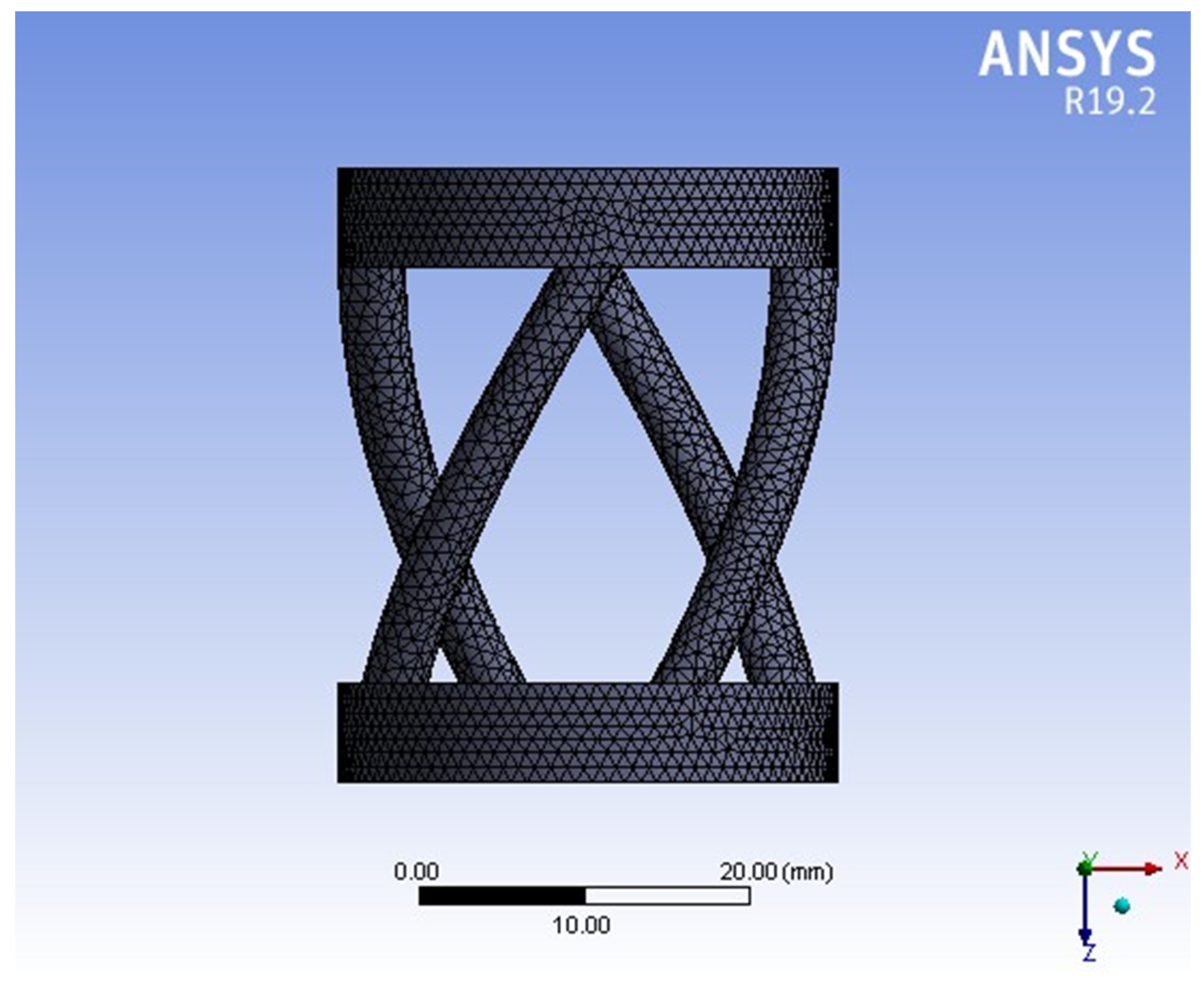
3. Applying MSL in the Numerical Method (Matlab) and FEM (Ansys Workbench)

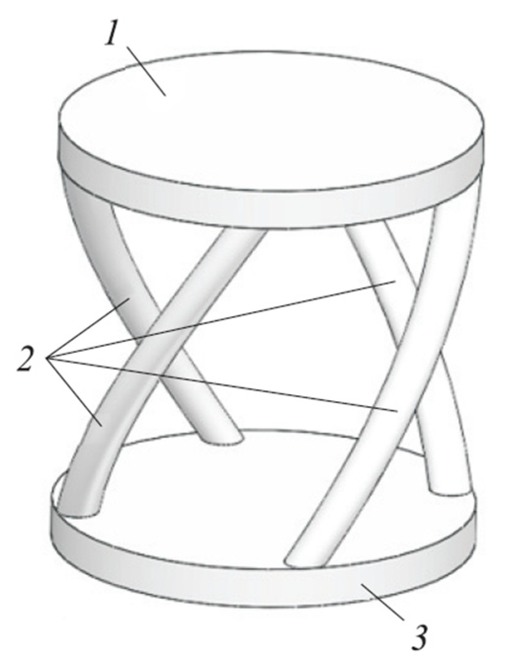
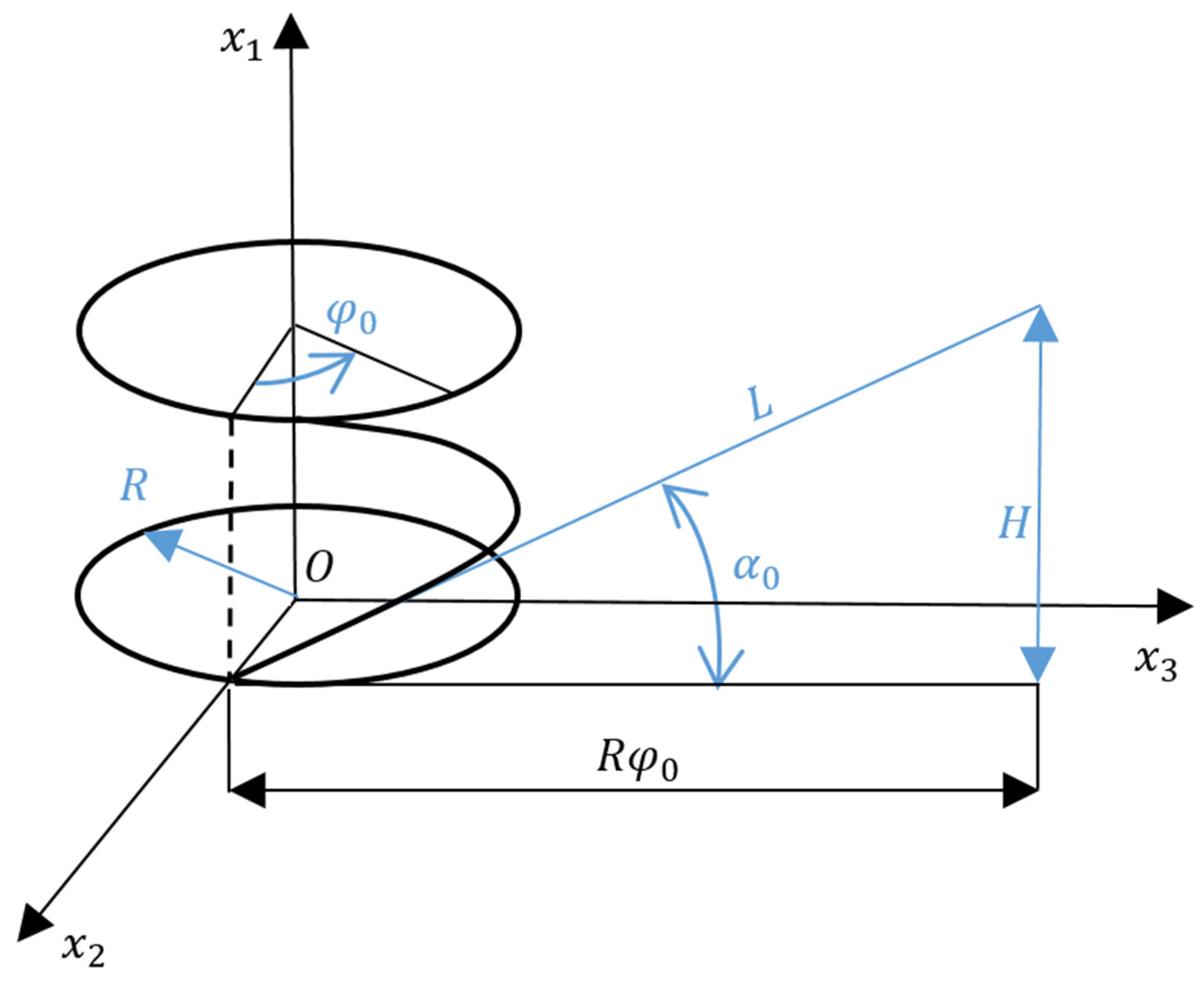
3.1. Designing the Model of Longitudinal–Transverse Transducers

This section considers the small vibrations of a spatial helical rod included in the longitudinal–torsional transducer of an ultrasonic medical instrument. An algorithm for determining the natural frequencies and waveforms of system vibrations by the method of initial parameters is developed. Based on this algorithm, the real elastic element of the longitudinal–transverse transducer is calculated using the mathematical package Matlab. The obtained natural frequencies ensure the operation of the ultrasound medical instrument in the resonant mode [31,32,33,34,35].
The helix angle α 0 is a constant value, so the sweep of a helix on a plane will be represented in the form of a straight line (see Figure 3). From here, we can get formulas relating to the angle lift of the helix ( α 0 ) , the length of the rod (L), the height of the rod (H), the radius of the circle (R), and the angle of twist ( φ 0 ):
α 0 = a r c t g H R φ 0 ; L = H sin α 0 .
The small free vibrations of a spatial rod in a dimensionless form have the following equation [36,37,38,39,40]:
n 1 2 u τ 2 Δ Q ε A Q A 1 Δ M A Κ Δ Q = 0 ; J 2 ϑ τ 2 Δ M ε A M A 1 Δ M A Κ Δ M A 1 Δ Q = 0 ; ϑ ε + A Κ ϑ A 1 Δ M = 0 ; u ε + A Κ u + A 1 ϑ = 0 ; Δ M = A Δ K ;
where
ε = s l ; τ = p 0 t ; p 0 = A 33 m 0 l 4 ; A ˜ i i = A i i A 33 ; M ˜ = M l A 33 ; Q ˜ = Q l 2 A 33 ; J ˜ i j = J i j F 0 l .
n 1 is the dimensionless linear mass of the rod; u is the displacement vector in the natural coordinate system; Δ Q is the vector of internal forces in section; A Q is the matrix of internal forces in a state of equilibrium; A 1 is the inverse stiffness matrix of the rod; Δ M is the vector of internal moments in the section; A κ is the matrix curvature in a state of equilibrium; J refers to the matrix moments of inertia of the section; ϑ is the vector of rotation angles in the natural coordinate system; A M is the matrix of internal moments in the state of equilibrium; A 1 is an auxiliary identity matrix; A refers to the stiffness matrix of the rod; Δ K is the matrix of curvature increments; A 33 is the torsional rigidity of the rod; m 0 is the mass per unit length of the rod; s is the axial coordinate of the section; p 0 is the factor of dimensionless time; t is time; A i i is the dimensional stiffness of the rod; i is the number of the natural coordinate axis; Q is the dimensional internal forces in the rod section; J i j refers to the moments of inertia of the section; j is the number of the natural coordinate axis; F 0 is the cross-sectional area.
We are looking for a solution to the system of Equation (21) in the following form:
Δ Q = Δ Q 0 ( ε ) e i λ τ ; Δ M = Δ M 0 ( ε ) e i λ τ ; ϑ = ϑ 0 ( ε ) e i λ τ ; u = u 0 ( ε ) e i λ τ ,
where Δ Q 0 is an array of increments of internal forces in the section of the rod; λ is the dimensionless natural frequency of the rod; Δ M 0 is an array of increments of internal moments; ϑ 0 is the vector of initial rotation angles of the section; u 0 is the vector of initial displacements of the section.
We obtain a system of ordinary differential equations:
d Q 0 d ε + A Q A 1 M 0 + A Κ Q 0 + λ 2 n 1 u 0 = 0 ; d M 0 d ε + ( A M A 1 + A Κ ) M 0 + A 1 Q + J λ 2 ϑ 0 = 0 ; d ϑ 0 d ε + A Κ ϑ 0 A 1 M 0 = 0 ; d u 0 d ε + A Κ u 0 + A 1 ϑ 0 = 0 .
The system of Equation (23) can be represented in the form of one vector–matrix equation:
d Ζ 0 d ε + B ( ε , λ ) Ζ 0 = 0 .
here
Ζ 0 = { Δ Q 0 Δ M 0 ϑ 0 u 0 } ; Β ( ε , λ ) = [ A Κ A Q A 1 0 λ 2 n 1 E A 1 A Μ A 1 J λ 2 0 0 A 1 A Κ 0 0 0 A 1 A Κ ] ,
where E is the elastic modulus of the rod.
The general solution of Equation (24) has the following form:
Z 0 ( ε ) = K ( ε ) C ,
where K( ε ) is the fundamental decision matrix; K(0) = E.
To obtain matrix K( ε ), we integrate the homogeneous Equation (24) twelve times with the following initial conditions:
Ζ 0 ( 1 ) = { 1 0 0 · · 0 } , Ζ 0 ( 2 ) = { 0 1 0 · · 0 } , , Ζ 0 ( 12 ) = { 0 0 0 · · 1 } .
Based on the rigid pinching of the rod at the ends, we have:
ϑ 1 = ϑ 2 = ϑ 3 = u 1 = u 2 = u 3 = 0 ;
where ϑ 1 , ϑ 2 , ϑ 3 , and u 1 , u 2 , u 3 are the components of the vectors ϑ and u, respectively.
This means that the six components of vector C will be equal to zero since the six components of Vector Z 0 are equal to zero:
c 7 = c 8 = = c 12 = 0 .
from here,
j = 1 6 k i j ( 1 ) c j = 0 ( i = 7 , 8 , , 12 ) ,
where k i j (1) refers to the elements of the fundamental matrix at ε = 1; c j is the jth component of Vector C.
Values λ j are the natural frequencies of the rod, in which the determinant of System (30) is equal to zero.
After determining the eigenfrequencies of rod λ i , we find from Equation (24) eigenfunctions Z 0 ( j ) satisfying the boundary conditions of the problem:
d Ζ 0 ( j ) d ε + Β ( ε , λ j ) Ζ 0 ( j ) = 0 .
Taking the last five equations from the system of linear Equation (30) for each value of natural frequency λ j , we find that the values c 2 ( j ) ,   c 3 ( j ) , …, c 6 ( j ) , depending on c 1 ( j ) , are determined up to a constant; parameter c 0 ( j ) can be set as equal to one [41,42,43,44,45].
After integrating Equation (31) with the obtained initial vector C j , we obtain the corresponding jth eigenmode of oscillation.
The material in this research is polyethylene. Its properties are shown by FEM (Ansys Workbench) in Table 1 and Table 2. Figure 4 shows the meshing of the model, and Figure 5 shows the six values (six modes) of vibration frequency by Ansys Workbench with different rods: λ F e m 1 ( f r e ) = 16 , 298   Hz ; λ F e m 2 ( f r e ) = 16 , 333   Hz ; λ F e m 3 ( f r e ) = 16 , 359   Hz ; λ F e m 4 ( f r e ) = 16 , 378   Hz ; λ F e m 5 ( f r e ) = 20 , 946   Hz ; λ F e m 6 ( f r e ) = 20 , 965   Hz .
We present the results of the modal analysis of a screw rod with the following initial data: rod’s height H = 36 mm; angle of twist φ 0 =   π /2; section’s diameter d = 4 mm; modulus of elasticity E = 2 × 10⁵ MPa (based on Table 2); Poisson’s ratio ν = 0.3 (based on Table 2); dimensionless factor p 0 = A 3 m . L 4 ; material density ρ = 7.85 × 10⁶ kg/mm3 (based on Table 1).
In solving the problem in the mathematical package Matlab, the natural frequencies of the rod were obtained: λ 1 = 23.3215; λ 2 = 25.1204; λ 3 = 26.9857. The natural frequencies of rod λ i are dimensionless quantities. To convert the dimensionless values of frequencies into hertz, they are multiplied by the dimensionless factor p 0 and divided by 2 π : λ N u m . M e t h o d 1 ( f r e ) = 20 , 835 (Hz); λ N u m . M e t h o d 2 ( f r e ) = 20 , 615 (Hz); λ N u m . M e t h o d 3 ( f r e ) = 20 , 547 (Hz).
For most ultrasonic instruments, the operating frequency of ultrasonic vibrations is close to 20 kHz [46,47,48,49,50]. On the other hand, the obtained natural oscillation frequencies are close to the working range by FEM (Ansys Workbench) and numerical method (Matlab). The most exact value Errorfre of FEM is 4.73 % at λ F e m 5 ( f r e ) , and the numerical method is 2.74 % at λ N u m . M e t h o d 2 ( f r e ) (see Table 3) (very good error).

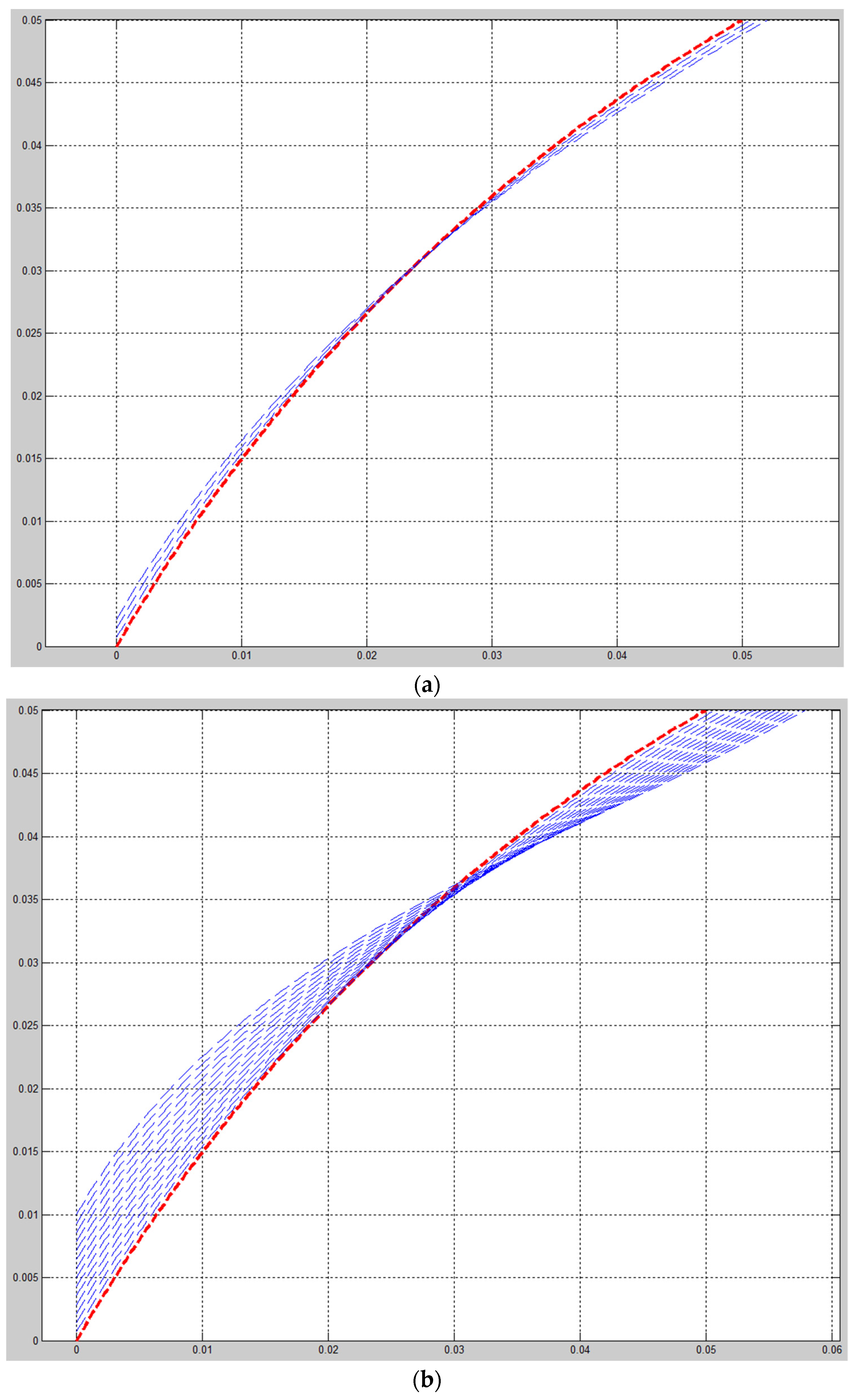
3.2. Calculating the Nonlinear Elastic Characteristic of Longitudinal–Transverse Transducers

Let us consider a numerical method that makes it possible to research the stress–strain state of a longitudinal–transverse transducer and obtain its nonlinear elastic characteristic.
The work aims to develop a mathematical model for calculating the stress–strain state of a flat, curved rod at large displacement.
For a flat, curved rod (see Figure 6), we determine the dependence of the vertical displacement (directed along Axis x 2 ), where u x 2 is the upper end of rod 2 on the horizontal displacement (co-directional with Axis x 1 ), and u x 1 is the lower end of rod 1.
We assume that the lower end of the rod moves strictly vertically along Axis x 2 , and its upper end moves in the guides strictly horizontally parallel to axis x 1 [51]. Further, we also assume that the ends are rigidly clamped; that is, they do not rotate relative to the attachment points. Noteworthily, we neglect the mass of the rod.
The following parameters are specified: height (H), starting angle ( β ) , and the angle’s rotation of the arc (φ).
The angles between local unit vector i 1 , co-directed with the global axis x 1 , and natural unit vector e 1 , directed tangentially to the arc circles, are defined by the following expressions:
At the beginning of the rod:
α 0 = π 2 β ;
At the end of the rod:
α 1 = π 2 ( β + φ ) .
Height:
H = R sin ( β + φ ) R sin β ,
where R is the radius of the circle.
From relation (23), we express the radius of the circle as follows:
R = H sin ( β + φ ) sin β .
We get a system from six equations:
d Q 1 d ε K 30 Q 2 = 0 ; d Q 2 d ε + K 30 Q 1 = 0 ; d M 3 d ε + Q 2 = 0 ; d ϑ 3 d ε 1 A 33 M 3 = 0 ; d u 1 d ε K 30 u 2 = 0 ; d u 2 d ε + K 30 u 1 ϑ 3 = 0 ,
where Q 1 and Q 2 are internal forces directed along axes x 1 and x 2 ; ε is the axial dimensionless coordinate; K 30 is the initial curvature of the rod axis; M 3 is the bending moment; ϑ 3 is the rotation angle of the cross-section of the rod; A 33 is the bending stiffness of the rod; u 1 and u 2 are the horizontal and vertical displacements of the rod’s cross-section.
Thus,
Δ P = 0
where Δ P —external concentrated force small increment.

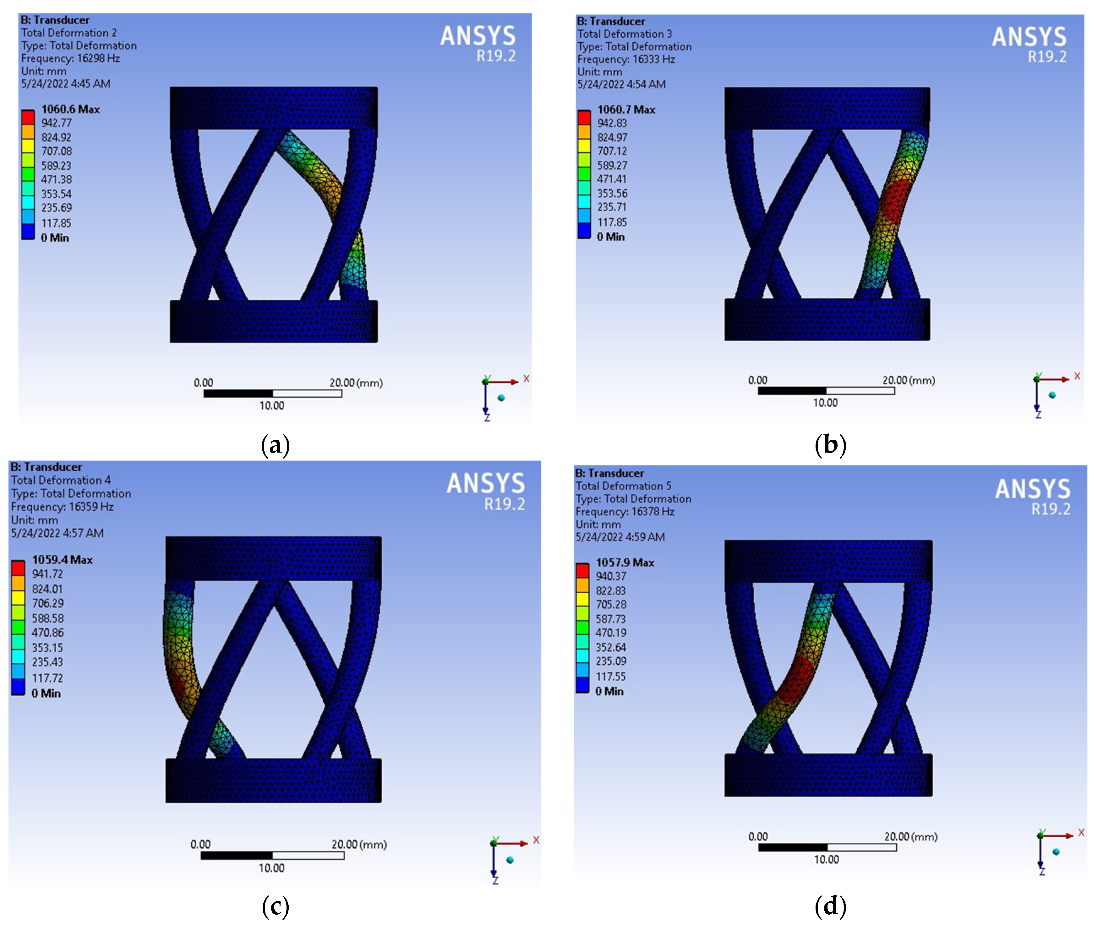
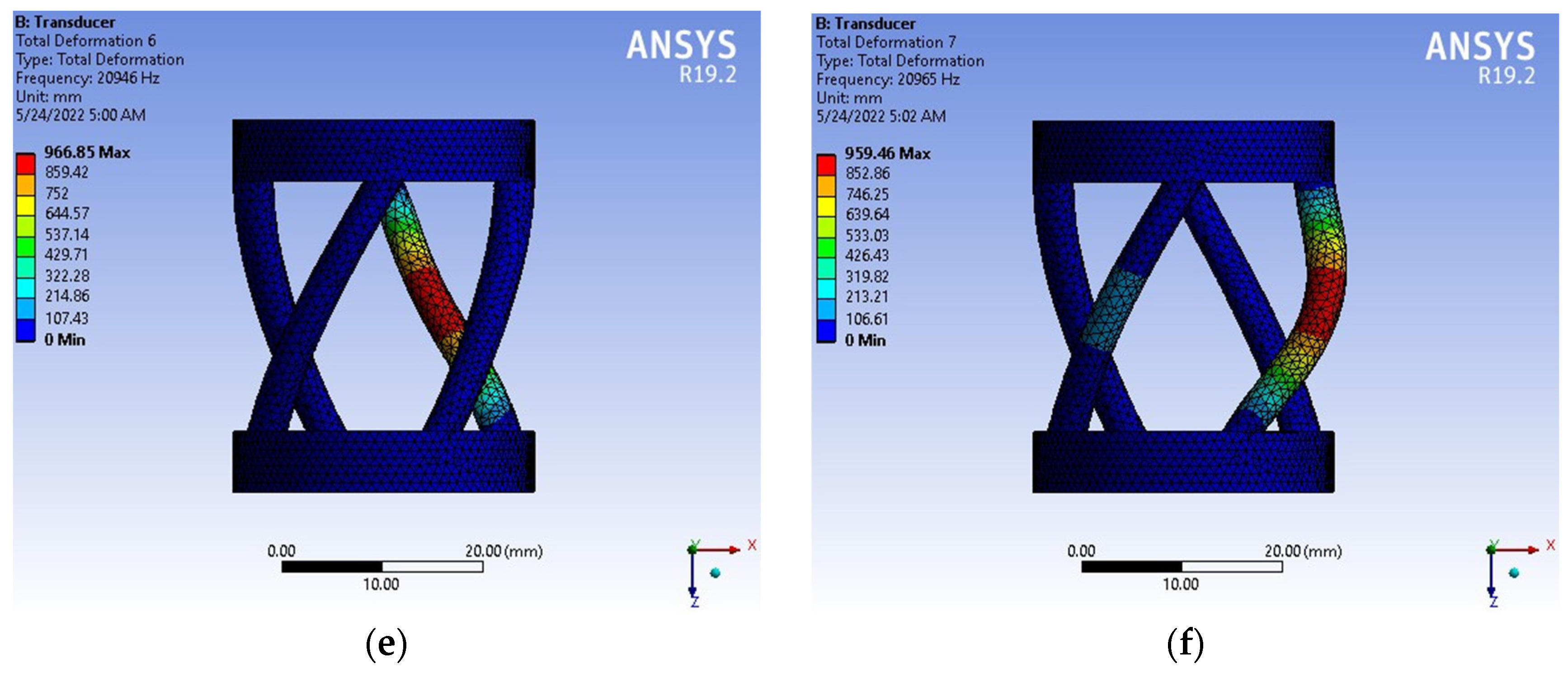
4. Results and Discussions

One of the methods for solving nonlinear problems is the MSL, in which linear equations describe each discrete increase in the load. For each mth step, the external force F(m) = kF, where m is the number of the loading step; k is a parameter that determines a part of the total load at each stage, and k = 1/n (n is the number of loading steps).
The system of equations for the first step of loading are as follows:
d Q 1 ( 1 ) d ε K 30 Q 2 ( 1 ) = 0 ; d Q 2 ( 1 ) d ε + K 30 Q 1 ( 1 ) = 0 ; d M 3 ( 1 ) d ε + Q 2 ( 1 ) = 0 ; d ϑ 3 ( 1 ) d ε 1 A 33 M 3 ( 1 ) = 0 ; d u 1 ( 1 ) d ε K 30 u 2 ( 1 ) = 0 ; d u 2 ( 1 ) d ε + K 30 u 1 ( 1 ) ϑ 3 ( 1 ) = 0 .
For each subsequent mth step of loading, the system of equations are as follows:
d Q 1 ( m ) d ε K 3 ( m 1 ) Q 2 ( m ) Q 2 ( m 1 ) Δ K 3 ( m ) = 0 ; d Q 2 ( m ) d ε + K 3 ( m 1 ) Q 1 ( m ) + Q 1 ( m 1 ) Δ K 3 ( m ) = 0 ; d M 3 ( m ) d ε + Q 2 ( m ) = 0 ; d ϑ 3 ( m ) d ε 1 A 33 M 3 ( m ) = 0 ; d u 1 ( m ) d ε K 3 ( m 1 ) u 2 ( m ) = 0 ; d u 2 ( m ) d ε + K 3 ( m 1 ) u 1 ( m ) ϑ 3 ( m ) = 0 ,
where
K 3 ( m 1 ) = K 30 + k = 2 m 1 Δ K 3 ( m ) = K 30 + k = 2 m 1 M 3 ( k ) A 33 ; Δ K 3 ( m ) = M 3 ( m ) A 33 ; Q j ( m 1 ) = k = 2 m 1 Δ Q j ( k ) .
The boundary conditions for the next step of the problem being solved should be considered.
With a dimensionless axial coordinate ε = 0, the lower end of the rod is rigidly clamped. Therefore, the angle of rotation ϑ 3 at the beginning of the section is zero [52].
The origin is set to move along axis x 1 . To solve the problem, it must be projected to the natural axis.
The rotation matrix for transitioning from the Cartesian coordinate system to the natural system has the following form:
L ( φ ) = [ cos φ sin φ sin φ cos φ ] ; { e 1 e 2 } = L ( φ ) { i 1 i 2 } .
The boundary conditions will be as follows:
ϑ 3 = 0 ; u 1 = Δ u 0 sin α 0 ; u 2 = Δ u 0 cos α 0 ,
where Δ u 0 is the small increment of displacement by the end of the rod.
With a dimensionless axial coordinate ε = 1, the upper end of the rod is rigidly clamped. Therefore, the angle of rotation ϑ 3 at the end of the segment is zero [53,54,55].
The upper end of the rod can only move horizontally in the guides. Thus, the following condition can be written as follows:
u x 2 = 0
The force directed along Axis x 1 must also be zero since the upper end of the rod can move freely in the x 2 direction:
Q x 2 = 0
These two boundary conditions are written in the Cartesian coordinate system. By projecting them into the natural axis at the end of the rod, we obtain the following algebraic expressions:
For displacements:
u x 2 = u 1 sin α 1 + u 2 cos α 1 ;
For forces:
Q 2 = Q 1 sin α 1 Q 2 cos α 1 .
Then, the boundary conditions will be as follows:
ϑ 3 = 0 ; u 1 sin α 1 + u 2 cos α 1 = 0 ; Q 1 sin α 1 Q 2 cos α 1 = 0 .
The resulting boundary conditions must be performed at each step of the solution by the MSL in the software complex Matlab since angles α 0 and α 1 remain unchanged throughout solving the problem.
We present the results for calculating a flat, curved rod with the following inputs: H = 50 mm; β = π /6; φ = π /6; section’s width b = 5 mm; section’s height h = 1 mm; Young’s module E = 2 × 10⁵ Mpa (based on Table 2).
The radius of the curvature calculated curved-linear rod, calculated by Formula (35): RAnalysis = 50 10 3 m sin ( π 6 + π 6 ) sin ( π 6 )   = 0.01566 m.
Solving a problem in the mathematical package, Matlab received graphs of the deformation axis of the rod at each step of the loading (see Figure 7 and Figure 8). Figure 7 shows the deformation process of the rod. Figure 8 shows graphs of the rod deformation axis: red curve 1 is the initial shape of the rod axis; black curve 2 is the shape of the rod axis at the last loading step; blue curves are the deformations of the rod. Maximum deformation of rod: uNum.Method(Max.def) = 983.54 mm (see Figure 8); uFem1(Max.def) = 1060.6 mm, uFem2(Max.def) = 1060.7 mm, uFem3(Max.def) = 1059.4 mm, uFem4(Max.def) = 1057.9 mm, uFem5(Max.def) = 966.85 mm, uFem6(Max.def) = 959.46 mm (see Figure 5). The values of deformation of the rod by FEM (Ansys Workbench) and numerical method (Matlab) have an insignificant difference. Maximum (%) error deformation: ErrorMax.def2  = 7.27 % and minimum (%) error deformation: ErrorMax.def5  = 1.73 % (see Table 4). That again shows that numerical method is a reliable method in simulation and computational engineering.
The dependence of the horizontal displacement of the upper end of the rod u x 2 from the vertical displacement of its lower end of the rod u x 1 (see Figure 9) is called the nonlinear elastic characteristic of the longitudinal–transverse transducer. The radius of the curvature calculated curved linear rod RNum.Method = 0.0165 m.
Error Non . Elas . Char   = R N u m . M e t h o d R A n a l y s i s R A n a l y s i s = 0.0165 0.01566 0.01566 × 100 % = 5.36 %
We obtained ErrorNon.Elas.Char = 5.36%, which proves that the algorithm for developing the MSL in the numerical method (Matlab) is correct.

5. Conclusions

The proposed algorithm for solving problems in rod mechanics with large displacements is approximate. However, according to the authors, its accuracy is quite acceptable for engineering practice. This method leverages its simple algorithmization for numerical calculation, in contrast to the solution of similar problems by the “zero” method and the parameter continuation methods. In addition, it should be noted that the geometry and the rod’s material properties can be easily varied, both in terms of the centerline and stiffness variability along the length. The above algorithm for the numerical research on the deep deformation of a flat rod is sufficient and can be easily adapted to solve problems involving static loading of structures in the form of spatially curvilinear rods of arbitrarily complex geometry.
For most ultrasonic instruments, the operating frequency of ultrasonic vibrations is close to 20 kHz. On the other hand, the received own oscillation frequencies are close to the working range. Changing the geometric characteristics of the screw rod and the material’s mechanical properties can achieve such conditions, under which a resonant mode will be implemented.
Using the MSL in the mathematical complex Matlab, a numerical calculation of the stress–strain state of a flat, curved rod at large displacements has been carried out. Based on the results obtained, a nonlinear elastic characteristic of the longitudinal–transverse transducer was constructed.

Author Contributions

Conceptualization, S.-C.H. and H.-D.N.; methodology, H.-D.N.; software, H.-D.N.; validation, S.-C.H. and H.-D.N.; formal analysis, H.-D.N.; investigation, S.-C.H.; resources, H.-D.N.; data curation, H.-D.N.; supervision, S.-C.H. All authors have read and agreed to the published version of the manuscript.

Funding

This research received no external funding.

Institutional Review Board Statement

Not applicable.

Informed Consent Statement

Not applicable.

Data Availability Statement

Data sharing is not applicable.

Acknowledgments

The authors acknowledge and thank the Ministry of Science and Technology of the Republic of China for their partial financial support of this study under Contract Number MOST 110-2622-E-992-009.

Conflicts of Interest

The authors declare no conflict of interest. The funders had no role in the design of the study; in the collection, analyses, or interpretation of data; in the writing of the manuscript, or in the decision to publish the results.

References

  1. Simo, J.C.; Tarnow, N.; Doblare, M. Non-linear dynamics of three-dimensional rods: Exact energy and momentum conservation algorithms. Int. J. Numer. Methods Eng. 1995, 38, 1431–1473. [Google Scholar] [CrossRef]
  2. Gerstmayr, J.; Shabana, A.A. Analysis of thin beams and cables using the absolute nodal coordinate formulation. Nonlinear Dyn. 2006, 45, 109–130. [Google Scholar] [CrossRef]
  3. Zhou, G.; Zhang, Y.; Zhang, B. The complex-mode vibration of ultrasonic vibration systems. Ultrasonics 2002, 40, 907–911. [Google Scholar] [CrossRef]
  4. Alnefaie, K. Lateral and longitudinal vibration of a rotating flexible beam coupled with torsional vibration of a flexible shaft. Int. J. Mech. Mechatron. Eng. 2018, 7, 884–891. [Google Scholar]
  5. Cardoni, A.; Harkness, P.; Lucas, M. Ultrasonic rock sampling using longitudinal-torsional vibrations. Phys. Procedia 2010, 3, 125–134. [Google Scholar] [CrossRef] [Green Version]
  6. Pani, S.; Senapati, S.; Patra, K.; Nath, P. Review of an Effective Dynamic Vibration Absorber for a Simply Supported Beam and Parametric Optimization to Reduce Vibration Amplitude. Int. J. Eng. Res. Appl. 2017, 7 Pt 3, 49–77. [Google Scholar] [CrossRef]
  7. He, B.; Rui, X.; Zhang, H. Transfer Matrix Method for Natural Vibration Analysis of Tree System. Math. Probl. Eng. 2012, 2012, 393204. [Google Scholar] [CrossRef] [Green Version]
  8. Allen, M.S.; Sracic, M.W.; Chauhan, S.; Hansen, M.H. Output-Only Modal Analysis of Linear Time Periodic Systems with Application to Wind Turbine Simulation Data. In Structural Dynamics and Renewable Energy; Proulx, T., Ed.; Springer: New York, NY, USA, 2011; Volume 1, pp. 361–374. [Google Scholar] [CrossRef] [Green Version]
  9. Allen, M.S.; Kuether, R.J.; Deaner, B.; Sracic, M.W. A numerical continuation method to compute nonlinear normal modes using modal reduction. In Proceedings of the 53rd AIAA/ASME/ASCE/AHS/ASC Structures, Structural Dynamics and Materials Conference, Honolulu, HI, USA, 23–26 April 2012; AIAA: Reston, VA, USA, 2012; pp. 9548–9567. [Google Scholar] [CrossRef] [Green Version]
  10. Structural Dynamics of Linear Elastic Single-Degree-of-Freedom (SDOF) Systems. Instructional Material Complementing FEMA 451, Design Examples. Available online: http://www.ce.memphis.edu/7119/PDFs/FEAM_Notes/Topic03StructuralDynamicsofSDOFSystemsNotes.pdf (accessed on 1 January 2020).
  11. Wen-Xi, H.; Xiao, X.Y.; Yun-Ling, J.; Dong-Fang, Y. Automatic segmentation method for voltage sag detection and characterization. In Proceedings of the 18th International Conference on Harmonics and Quality of Power (ICHQP), Ljubljana, Slovenia, 13–16 May 2018; IEEE: New York, NY, USA, 2018; pp. 1–5. [Google Scholar] [CrossRef]
  12. Zilletti, M.; Elliott, S.J.; Rustighi, E. Optimisation of dynamic vibration absorbers to minimise kinetic energy and maximise internal power dissipation. J. Sound Vib. 2012, 331, 4093–4100. [Google Scholar] [CrossRef] [Green Version]
  13. Kulterbaev, K.P.; Baragunova, L.A.; Shogenova, M.M.; Shardanova, M.A. The Solution of a Spectral Task on Variable Section Compressed Beams Oscillations by Numerical Methods Materials. Sci. Forum 2019, 974, 704–710. [Google Scholar] [CrossRef]
  14. Kulterbaev, K.P.; Alokova, M.H.; Baragunova, L.A. Mathematical modeling of flexural oscillations of a vertical rod of variable section. News High. Educ. Inst. N.-Caucasion Region. Techn. Sci. 2015, 4, 100–106. [Google Scholar]
  15. Gavryushin, S.S.; Baryshnikova, O.O.; Boriskin, O.F. Numerical Analysis of Structural Elements of Machines and Devices; BMSTU Publishing: Moscow, Russia, 2014; p. 479. [Google Scholar]
  16. Kikvidze, O.G.; Kikvidze, L.G. Large Displacements of Thermoelastic Rods during Plane Bending. In Problems of Applied Mechanics; Publishing House “Committee of IFToMM of Georgia”: Tbilisi, Georgia, 2001; Chapter 4; pp. 73–77. [Google Scholar]
  17. Kikvidze, O.G.; Kikvidze, L.G. The geometrically nonlinear problem of bending thermoelastic rods. In Collection of International Symposium “Problems of Thin-Walled Spatial Structures”; Georgian Technical University: Tbilisi, Georgia, 2007; pp. 28–31. [Google Scholar]
  18. Kikvidze, O.G. Large displacements of thermoelastic rods during bending. In Problems of Mechanical Engineering and Machine reliability; RAS: Moscow, Russia, 2003; Chapter 1; pp. 49–53. [Google Scholar]
  19. Bîrsan, M.; Altenbach, H. Theory of thin thermoelastic rods made of porous materials. Arch. Appl. Mech. 2011, 81, 1365–1391. [Google Scholar] [CrossRef]
  20. Starovoitov, E.I.; Leonenko, D.V.; Tarlakovskii, D.V. Thermal-force deformation of a physically nonlinear three-layer stepped rod. J. Eng. Phys. Thermophys. 2016, 89, 1582–1590. [Google Scholar] [CrossRef]
  21. Baisarova, G.; Brzhanov, R.; Kikvidze, O.G.; Lahno, V. Computer simulation of large displacements of thermoelastic rods. J. Theor. Appl. Inf. Technol. 2019, 97, 4188–4201. [Google Scholar]
  22. Svetlitskii, V.A. Construction Machinery Mechanic. In Mechanics Rods; Fizmatlit Publ.: Moscow, Russia, 2009; Volume 1, p. 408. [Google Scholar]
  23. Bednarcyk, B.A.; Aboudi, J.; Arnold, S.M.; Pineda, E.J. A multiscale two-way thermomechanically coupled micromechanics analysis of the impact response of thermo-elastic-viscoplastic composites. Int. J. Solids Struct. 2019, 161, 228–242. [Google Scholar] [CrossRef]
  24. Qiu, B.; Kan, Q.; Kang, G.; Yu, C.; Xie, X. Rate-dependent transformation ratcheting-fatigue interaction of super-elastic NiTi alloy under uniaxial and torsional loadings: Experimental observation. Int. J. Fatigue 2019, 127, 470–478. [Google Scholar] [CrossRef]
  25. Rossmann, L.; Sarley, B.; Hernandez, J.; Kenesei, P.; Köster, A.; Wischek, J.; Almer, J.; Maurel, V.; Bartsch, M.; Raghavan, S. Method for conducting in situ high-temperature digital image correlation with simultaneous synchrotron measurements under thermomechanical conditions. Rev. Sci. Instruments 2020, 91, 033705. [Google Scholar] [CrossRef] [PubMed]
  26. Hu, Y.-J.; Zhou, H.; Zhu, W.; Zhu, J. A thermally-coupled elastic large-deformation model of a multilayered functionally graded material curved beam. Compos. Struct. 2020, 244, 112241. [Google Scholar] [CrossRef]
  27. Frantık, P. Simulation of the stability loss of the von Mises truss in an unsymmetrical stress state. Eng. Mech. 2007, 14, 155–161. Available online: http://www.engineeringmechanics.cz/pdf/14_3_155.pdf (accessed on 1 January 2020).
  28. Greco, M.; Vicente, C.E.R. Analytical solutions for geometrically nonlinear trusses. Rev. Esc. Minas 2009, 62, 205–214. [Google Scholar] [CrossRef] [Green Version]
  29. Cвeтлицкий, B.A.; Hapaйкин, O.C. Уnpyгиe элeмeнты мaшин; Maшинocтpoeниe: Moscow, Russia, 1989; p. 29. (In Russian) [Google Scholar]
  30. Kala, Z. Stability of von-Misses Truss with Initial Random Imperfections. Procedia Eng. 2017, 172, 473–480. [Google Scholar] [CrossRef]
  31. Gacesa, M.; Jelenic, G. Modified fixed-pole approach in geometrically exact spatial beam finite elements. Finite Elem. Anal. Des. 2015, 99, 39–48. [Google Scholar] [CrossRef]
  32. Kalina, M. Stability Problems of Pyramidal von Mises Planar Trusses with Geometrical Imperfection. Int. J. Theor. Appl. Mech. 2016, 1, 118–123. Available online: https://www.iaras.org/iaras/filedownloads/ijtam/2016/009-0018.pdf (accessed on 25 April 2022).
  33. Ligarò, S.S.; Valvo, P.S. Large Displacement Analysis of Elastic Pyramidal Trusses. Int. J. Solids Struct. 2006, 43, 4867–4887. Available online: https://www.researchgate.net/profile/Paolo_Valvo/publication/229292690 (accessed on 1 January 2020). [CrossRef]
  34. Mikhlin, Y.V. Nonlinear normal vibration modes and their applications. In Proceedings of the 9th Brazilian Conference on Dynamics Control and their Applications, Serra Negra, Brazil, 7–11 June 2010; pp. 151–171. Available online: https://www.sbmac.org.br/dincon/trabalhos/PDF/invited/68092.pdf (accessed on 25 April 2022).
  35. Jelenic, G.; Crisfield, M.A. Geometrically exact 3D beam theory: Implementation of a strain-invariant finite element for static and dynamics. Comput. Methods Appl. Mech. Eng. 1999, 171, 141–171. [Google Scholar] [CrossRef]
  36. Shabana, A.A.; Yakoub, R.Y. Three dimensional absolute nodal coordinate formulation for beam elements: Theory. ASME J. Mech. Des. 2001, 123, 606–613. [Google Scholar] [CrossRef]
  37. Simo, J.C.; Vu-Quoc, L. A three-dimensional finite-strain rod model. Part II: Geometric and computational aspects. Comput. Methods Appl. Mech. Eng. 1986, 58, 79–116. [Google Scholar] [CrossRef]
  38. Papa, E.; Jelenic, G.; Gacesa, M. Configuration-dependent interpolation in higher-order 2D beam finite elements. Finite Elem. Anal. Des. 2014, 78, 47–61. [Google Scholar] [CrossRef]
  39. Cвeтлицкий, B.A. мexaникa cтepжнeй. Динaмикa; Maшинocтpoeниe: Moscow, Russia, 1987; p. 55. (In Russian) [Google Scholar]
  40. Xiao, N.; Zhong, H. Non-linear quadrature element analysis of planar frames based on geometrically exact beam theory. Int. J. Non-Lin. Mech. 2012, 47, 481–488. [Google Scholar] [CrossRef]
  41. Makinen, J. Total Lagrangian Reissner’s geometrically exact beam element without singularities. Int. J. Numer. Methods Eng. 2007, 70, 1009–1048. [Google Scholar] [CrossRef]
  42. Zacny, K.; Bar-Cohen, Y.; Brennan, M.; Briggs, G.; Cooper, G.; Davis, K.; Dolgin, B.; Glaser, D.; Glass, B.; Gorevan, S.; et al. Drilling Systems for Extraterrestrial Subsurface Exploration. Astrobiology 2008, 8, 665–706. [Google Scholar] [CrossRef] [Green Version]
  43. Bar-Cohen, Y.; Sherrit, S.; Dolgin, B.; Bridges, N.; Bao, X.; Chang, Z.; Yen, A.; Saunders, R.; Pal, D.; Kroh, J.; et al. Ultrasonic/sonic driller/corer (USDC) as a sampler for planetary exploration. In Proceedings of the 2001 IEEE Aerospace Conference, Big Sky, MT, USA, 10–17 March 2001. [Google Scholar] [CrossRef] [Green Version]
  44. Bar-Cohen, Y.; Bao, X.; Chang, Z.; Sherrit, S. An ultrasonic sampler and sensor platform for in situ astrobiological exploration. In Proceedings of the SPIE Smart Structures Conference, San Diego, CA, USA, 2–6 March 2003; Volume 5056, pp. 457–465. [Google Scholar] [CrossRef] [Green Version]
  45. Badescu, M.; Stroescu, S.; Sherrit, S.; Aldrich, J.; Bao, X.; Bar-Cohen, Y.; Chang, Z.; Hernandez, W.; Ibrahim, A. Rotary hammer ultrasonic/sonic drill system. In Proceedings of the IEEE International Conference on Robotics and Automation, Pasadena, CA, USA, 19–23 May 2008; pp. 602–607. [Google Scholar] [CrossRef]
  46. Tsujino, J. Ultrasonic motor using a one-dimensional longitudinal-torsional vibration converter with diagonal slits. Smart Mater. Struct. 1997, 7, 345–351. [Google Scholar] [CrossRef]
  47. Ohnishi, O.; Myohga, O.; Uchikawa, T.; Tamegai, M.; Inoue, T.; Takahashi, S. Piezoelectric ultrasonic motor using longitudinal-torsional composite resonance vibration. IEEE Trans. Ultrason. Ferroelectr. Freq. Control 1993, 40, 687. [Google Scholar] [CrossRef] [PubMed]
  48. Harkness, P.; Cardoni, A.; Lucas, M. Vibration considerations in design of an ultrasonic driller/corer for planetary rock sampling. In Proceedings of the ISMA 2008: International Conference on Noise and Vibration Engineering, Leuven, Belgium, 15–17 September 2008. [Google Scholar]
  49. Harkness, P.; Cardoni, A.; Lucas, M. An ultrasonic corer for planetary rock sample retrieval. In Proceedings of the 7th International Conference on Modern Practice in Stress and Vibration Analysis, Cambridge, UK, 8–10 September 2009. [Google Scholar] [CrossRef]
  50. Lobontiu, N.; Paine, J.S.; Garcia, E.; Goldfarb, M. Design of symmetric conic-section flexure hinges based on closed-form compliance equations. Mech. Mach. Theory 2002, 37, 477–498. [Google Scholar] [CrossRef]
  51. Zhu, Z.; Zhou, X.; Wang, R.; Liu, Q. A simple compliance modeling method for flexure hinges. Sci. China Technol. Sci. 2015, 58, 56–63. [Google Scholar] [CrossRef]
  52. Zhu, Z.; Zhou, X.; Liu, Q.; Zhao, S. Multi-objective optimum design of fast tool servo based on improved differential evolution algorithm. J. Mech. Sci. Technol. 2011, 25, 3141–3149. [Google Scholar] [CrossRef]
  53. Gao, W.; Araki, T.; Kiyono, S.; Okazaki, Y.; Yamanaka, M. Precision nano-fabrication and evaluation of a large area sinusoidal grid surface for a surface encoder. Precis. Eng. 2003, 27, 289–298. [Google Scholar] [CrossRef]
  54. Liu, C.; Ta, D.; Hu, B.; Le, L.H.; Wang, W. The analysis and compensation of cortical thickness effect on ultrasonic backscatter signals in cancellous bone. J. Appl. Phys. 2014, 116, 124903. [Google Scholar] [CrossRef]
  55. Fontes-Pereira, A.J.; Matusin, D.; Rosa, P.; Schanaider, A.; von Krüger, M.; Pereira, W. Ultrasound method applied to characterize healthy femoral diaphysis of Wistar rats in vivo. Braz. J. Med. Biol. Res. 2021, 47, 403–410. [Google Scholar] [CrossRef] [Green Version]
Figure 1. Structure and principle of operation of the longitudinal–transverse transducer: (1) linear displacement entry platform; (2) screw rods; (3) exit platform, performing rotary displacement.
Materials 15 04002 g001
Figure 2. Relationship between the center angle φ ( s ) and angle ϑ 30 (s).
Materials 15 04002 g002
Figure 3. Scheme for calculating the helix.
Materials 15 04002 g003
Figure 4. The meshing of the model.
Materials 15 04002 g004
Figure 5. Values of vibration frequency for six modes of model. (a) Mode one. (b) Mode two. (c) Mode three. (d) Mode four. (e) Mode five. (f) Mode six.
Materials 15 04002 g005aMaterials 15 04002 g005b
Figure 6. Scheme for determining displacements flat curved rod.
Materials 15 04002 g006
Figure 7. Graphs of the rod deformation axis: (a) Beginning process; (b) Quarter process; (c) Half process; (d) Three-fourths process; (e) End process.
Materials 15 04002 g007aMaterials 15 04002 g007bMaterials 15 04002 g007c
Figure 8. Graphs of the rod deformation axis: 1 is the initial shape of the rod axis; 2 is the shape of the rod axis at the last loading step.
Materials 15 04002 g008
Figure 9. Nonlinear elastic characteristic longitudinal–transverse transducer.
Materials 15 04002 g009
Table 1. Structural steel’s constants by FEM (Ansys Workbench).
Density7.85 × 106 kg/mm3
Table 2. Structural steel’s isotropic elasticity by FEM (Ansys Workbench).
Young’s Modulus (MPa)Poisson’s RatioTensile Yield Strength (MPa)Tensile Ultimate Strength (MPa)
2 × 1050.3250460
Table 3. Value frequencies of vibrations by FEM and the numerical method, and the reality in medicine.
Reality in Medicine (kHz) [48]20
FEM   λ F e m 1 ( f r e )   ( kHz ) 16.298 Error fre = 20 16.298 20 × 100 % = 18.51 %
FEM   λ F e m 2 ( f r e )   ( kHz ) 16.333 Error fre = 20 16.333 20 × 100 % = 18.36 %
FEM   λ F e m 3 ( f r e )   ( kHz ) 16.359 Error fre = 20 16.359 20 × 100 % = 18.21 %
FEM   λ F e m 4 ( f r e )   ( kHz ) 16.378 Error fre = 20 16.378 20 × 100 % = 18.11 %
FEM   λ F e m 5 ( f r e )   ( kHz ) 20.946 Error fre = 20.946 20 20 × 100 % = 4.73 %
FEM   λ F e m 6 ( f r e )   ( kHz ) 20.965 Error fre = 20.965 20 20 × 100 % = 4.83 %
Numerical   method   λ N u m . M e t h o d 1 ( f r e ) (kHz) 20.835 Error fre = 20.835 20 20 × 100 % = 4.18 %
Numerical   method   λ N u m . M e t h o d 2 ( f r e ) (kHz) 20.615 Error fre = 20.615 20 20 × 100 % = 3.08 %
Numerical   method   λ N u m . M e t h o d 3 ( f r e ) (kHz) 20.547 Error fre = 20.547 20 20 × 100 % = 2.74 %
Table 4. Values of maximum deformation by FEM and numerical method.
FEM (Ansys) (mm)Numerical Method (Matlab) (mm)(%) ErrorMax.def
1060.6 Error Max . def 1   = 1060.6 983.54 1060.6 × 100 % = 7.27 %
1060.7 Error Max . def 2   = 1060.7 983.54 1060.7 × 100 % = 7.27 %
1059.4983.54 Error Max . def 3   = 1059.4 983.54 1059.4 × 100 % = 7.16 %
1057.9 Error Max . def 4   = 1057.9 983.54 1057.9 × 100 % = 7.03 %
966.85 Error Max . def 5   = 966.85 983.54 966.85 × 100 % = 1.73 %
959.46 Error Max . def 6   = 983.54 959.46 959.46 × 100 % = 2.50 %
Publisher’s Note: MDPI stays neutral with regard to jurisdictional claims in published maps and institutional affiliations.

