Abstract
The paper deals with the problem of stress concentration at the weld toe of a plate T-joint subjected to axial, bending, and shearing loading modes. Theoretical stress concentration factors were obtained from numerical simulations using the finite element method for several thousand geometrical cases, where five of the most important geometrical parameters of the joint were considered to be independent variables. For each loading mode—axial, bending, and shearing—highly accurate closed form parametric expression has been derived with a maximum percentage error lower than 2% with respect to the numerical values. Validity of each approximating formula covers the range of dimensional proportions of welded plate T-joints used in engineering applications. Two limiting cases are also included in the solutions—when the weld toe radius tends to zero and the main plate thickness becomes infinite.
1. Introduction
Welded T-connections are commonly used engineering structures. Their significant advantage lies in low costs of production due to the use of simple elements, like tubes of circular or rectangular cross sections and plates, usually connected by welding. There are many types of such joints produced in various configurations: as tubular, tubular-plate, and plate couples. The fatigue failure of welded structural components subjected to cyclic loads is the most frequent cause of damage, which begins at critical zones where stress concentration occurs [1]. Various standards and recommendations presented in References [2,3,4,5,6,7] are very helpful in designing welded structures.
Stress concentration factor (SCF) values determined for the known geometrical and loading conditions are of great importance in fatigue design because they enable relating the loading history to the critical zone of the structure. Some examples of fatigue analysis in tubular joints applied to various types of structures and devices are given in References [8,9,10,11,12] where stress concentration plays a key role. Fatigue damage analysis considering crack initiation and propagation processes in welded T-joints was published in References [13,14,15]. Numerous formulas of stress concentration factors for various types of welded T-joints, based on the finite and boundary element analyses, were presented in References [16,17,18,19,20].
Some important phenomena associated with welding processes consist of a random character of key geometrical parameters influencing the SCF value. In such cases, appropriate statistic data obtained directly from real structures and regarding changed values and shapes of weldments are necessary. Examples of such data in the form of histograms can be found in the literature [21,22,23,24,25]. Various types of the weld face geometry—plane, convex, or concave—may be obtained during manufacturing, which generally depend on the welding method, position, and parameters of the process, e.g., welding speed, current, etc. Some examples of real weld shapes and profiles influencing SCF values in cases of as-welded and intentionally improved weld toe zones are also given in References [25,26,27,28,29]. Many techniques have also been developed to improve the endurance limit and reliability of the structure (grinding, milling, re-melting techniques, etc.) [30]. Each process produces specific radii influencing local stress concentration.
The application of the known parametric formulas in fatigue design encounters some difficulties arising from their accuracy, range of validity, and different ways of defining SCF. On the other hand, assessment of fatigue life requires high accuracy of SCF solutions and should cover the whole range of values of all key parameters influencing SCFs.
The present study deals with determination of stress concentration factors for non-load carrying welded plate T-joints subjected to axial, bending and shearing loading modes. The main objective was to develop highly accurate SCF formulas of a wide ranging validity, including two limiting cases: when the toe radius ρ tends to zero and when the main plate thickness t becomes infinite.
2. Methodology
2.1. General Assumptions
Five key geometrical parameters—ρ, a, θ, t, and T—have been selected and considered as independent variables, where t and T represent the main and attachment plate thickness, respectively, ρ is the weld toe radius, θ indicates the weld angle, and a is the weld throat thickness defined here as the shortest distance between the joint root and the weld face. Leg length parameters, h and hp, characterizing the weld size, are also used in the literature, e.g., in References [16,17,18]. Shape and geometrical dimensions of a plate T-joint, as well as three loading modes considered in the present work, are depicted schematically in Figure 1. Small circles drawn symmetrically at the weld toe zone indicate locations of the maximum stresses.
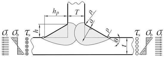
Figure 1.
Geometrical parameters and loading modes of the plate T-joint.
The present analysis considered the following assumptions.
- Joint material is linear elastic, isotropic, and homogeneous.
- Elastic properties of the weld material and the base material, represented by elastic constants, are the same.
- The welded joint is free from residual stresses, structural irregularities, and imperfections, including lack of penetration defects.
- Both welds are symmetrical with respect to the axis of the attachment plate, which is perpendicular to the main plate.
- Weld faces are plane and contour of the weldment is smooth with a transition toe radius ρ > 0.
- External load – axial, bending, and shearing – is applied at the opposite sides of the main plate sufficiently far from the welds.
- Small deformations occur in the whole body.
- Five geometrical parameters: ρ, a, θ, t, and T are considered as independent variables varying in the following ranges: 0 < ρ/a ≤ 1.3, 0 < a/t ≤ 1.3, 1 ≤ T/a ≤ 4, and 30° ≤ θ ≤ 60°.
- Stress concentration factors for axial, bending, and shearing loads are defined as Ktt = σ1max/σt, Ktb = σ1max/σb, and Kts = τmax/τs, respectively.
Theoretical stress concentration factor SCF is valid for linear-elastic, homogeneous, and isotropic materials as well as bodies of defined geometry, loading and displacement boundary conditions. Any departure from these assumptions, as material anisotropy or geometrical irregularities (flaws, imperfections, etc.) may significantly change the stress distribution in the body, including the maximum stress value at the notch root.
The aim of the work was to obtain SCF approximating formulae covering possible proportions between geometrical parameters of the T-joint used in engineering practice. For this reason, the supposed margin for the normalized parameters was very wide. The weld toe radius ρ 1.3 times larger than the weld throat may be considered useless for practical applications, but such a limiting value can guarantee that all smaller radii fall into the range of application. The second case when a/t→0 may also take place in engineering applications while a relatively thin plate is welded to a very thick main plate.
2.2. General Approach
The procedure of reaching main objectives of the present study consisted of several steps. First, conveniently defined new geometrical parameters had to be specified. Due to the fact that SCF values do not vary when all dimensions of the body proportionally change, the following normalized non-dimensional quantities were introduced.
In this way, four independent variables X, Y, Z, and θ, containing the five key dimensions of the joint, were taken into consideration. The upper weld toe radius, ρ1, shown in Figure 1, was chosen as equal to 0.1a and had no influence on stress concentration factors. The second step consisted of numerical modelling of the joint using the finite element method, where mutual proportions between the basic joint dimensions systematically changed. In this way, several thousands of SCF values, covering the assumed range of validity, were determined. More detailed information on the numerical modelling and SCF calculating procedures are presented in the next section. The third step of the approach consisted of choosing a general form of the mathematical representation of SCFs’ approximating functions. An expression applied in the present study was similar to that presented by the authors in Reference [31], where a cruciform joint of θ = 45°, subjected to tensile and bending loads, was analysed. However, the problem considered in the present work was more general than the previous one because the weld angle θ varied in the range of 30–60°, increasing the number of variables in the parametric formula. In the numerical Finite Element Method (FEM) modelling, the weld angle θ was changed by 2.5° and the whole calculating procedure, carried out for a given angle, had to be repeated 12 times. Hence, a general form of the approximating function is given by Equation (4).
where a singular term Xn accounts for the stress concentration effects when ρ→0. The function P(X,Y,θ,Z0), represented by polynomials, can be derived from numerical SCF solutions normalized with respect to the singular term, Kt/Xn for different X, Y, and θ, while Z = Z0. Equation (4) indicates that the P function cannot directly relate SCF to Z because it is derived for a particular, arbitrarily chosen value of Z = Z0. For this reason, the additional correction function is κ(X,Y,Z,θ,Z0), satisfying Equation (5),
was necessary to account for the relative stiffener thickness on SCF. In other words, the function κ can be interpreted as a multiplier, which enables us to calculate SCF for any value of Z with respect to the one corresponding to Z0, for the known parameters X, Y, and θ.
The exponent n, denoted as ns for shearing load, is necessary to describe stress concentration effects when the weld toe radius tends to zero. In References [31,32], it was proven that the correct n values are the same as the stress field singularity exponents corresponding to the characteristic angle of the sharp corner [33], into which the weld toe region is converted while the weld toe radius ρ tends to zero. According to Reference [32], numerical values of the exponent n can be calculated for axial and bending load, using Equation (6),
which is valid in the range of 0 ≤ θ ≤ π/2 with an accuracy of five significant digits.
For anti-plane deformation produced by the shearing load, the exact value of the exponent ns equals:
where θ is in radians.
The next step of the procedure consisted of approximating the P(X,Y,Z0,θ) function to the normalized numerical SCF data using the least squares method. After particular constants (coefficients and exponents) of the P function were determined, the approximation accuracy was verified. In this way, one part of the solution, where Z = Z0, was completed. The final step of the present approach consisted of finding unknown coefficients and exponents of the correction function κ(X,Y,Z,θ,Z0) accounting for the influence of Z values on SCFs. After performing the second validation of the full solution including κ, the close form approximating functions for calculating SCFs were determined. The whole procedure was consecutively repeated for each loading mode.
3. Numerical FEM Modelling and Some SCFs’ Results
3.1. Tensile and Bending Load
Systematic numerical modelling of plate T-joints was carried out by using the Finite Element Method (FEM) incorporated in the ANSYS 19 Multiphysics program. The PLANE182 finite elements that were used were defined by four nodes having 2 degrees of freedom at each node. The elastic material constants were assumed to be similar to those for steel, where Young’s modulus E = 210 GPa and Poisson’s ratio ν = 0.3. However, according to the theory of elasticity, stress field in the body and SCF values do not depend on the elastic constants of the material in all cases modeled. Loading and displacement boundary conditions imposed on one half of the body, as well as its shape, are shown in Figure 2. According to the principle of de Saint Venant, the minimum length of the main plate measured from the weld toe was about 4.5t. This value was confirmed by conducting preliminary numerical tests.
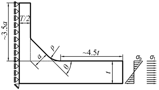
Figure 2.
Basic geometrical parameters and boundary conditions of the numerical FEM model for tensile and bending loads.
Approximately 820,000 finite elements were used for each geometrical case of the modelled T-joint. Special attention was paid to the finite element mesh density at the weld toe zone, where high values of the stress gradients occur. For this reason, the dimensional ratio of neighbouring finite elements was about 1.2 and approximately 40 to 70 finite elements were used along the weld toe circular arc, as described by the radius ρ. One example of a finite element mesh is shown in Figure 3.
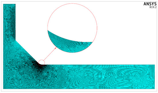
Figure 3.
Example of a finite element mesh for θ = 45°, while X = 0.25, Y = 0.415, and T/t = 1.
An example of the solution obtained for the tensile load for the nominal uniform stress σt = 1 MPa applied over the right end of the body is shown in Figure 4. The first principal stress results offer the most convenient representation because the particular value of the SCF is directly accessible. Therefore, the nominal stress in all numerical models was always equal to one.
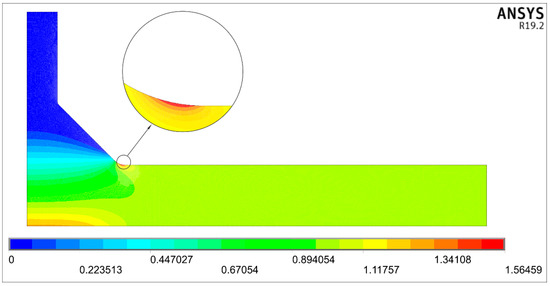
Figure 4.
Distribution of the first principal stress σ1 for σt = 1 MPa, while θ = 45°, X = 0.25, Y = 0.415, and T/t = 1.
In the presented case, the maximum principal stress σ1max equals 1.56459 MPa, which is directly seen on the scale below the picture. This value is also interpreted as the stress concentration factor Ktt.
3.2. Shearing Load
The formulation of two-dimensional problems for the anti-plane state of deformation is different than for in-plane loading modes. In the case of the anti-plane problem, only one displacement coordinate W in each point is sufficient to describe deformation of the body and W(x,y) may be treated as a scalar potential function ψ(x,y). Therefore, a problem in an anti-plane state of deformation may be considered as a boundary value problem governed by Laplace’s equation, represented in Cartesian coordinates by Equation (8).
which is valid in the whole body and satisfies boundary conditions along the surrounding contour. The fact that the same relationship also holds for the temperature field Ttemp(x,y) in plane steady-state heat conduction problems leads to the conclusion that thermal analogy may be used to obtain solutions of stress concentration factors for an anti–plane state of deformation. A more detailed description of this approach can be found in Reference [32] where SCFs for butt-welded plates subjected to shearing load were determined using FEM.
In the present analysis, the ANSYS 19 Multiphysics program with a Thermal module and PLANE55 finite element was used. A PLANE55 finite element is defined by four nodes with a single degree of freedom corresponding to the temperature at each node. Meshing of the modelled area was the same as in the previous cases for tensile and bending loads for identical joint geometry. The shape of the modelled body as well as mixed boundary conditions are shown in Figure 5.
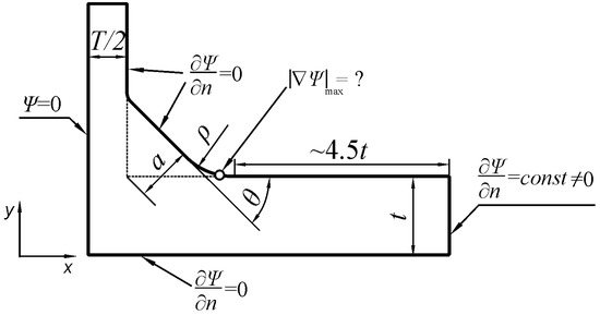
Figure 5.
Shape and boundary conditions of the numerical FEM model for shearing load.
Nominal uniform heat flux qnom = 1 W/m2 was applied over the right-hand edge of the body, while zero temperature was applied to the left end along the plane of symmetry of the joint. Since the upper face and the lower face of the joint are free from external shearing loads, they have to be insulated in the thermal model. It is clear that the shear stress components, τxz and τyz, given by Equation (9):
and related to the partial derivatives of the potential function W(x,y) in particular directions, are proportional to the corresponding heat flux components, qx and qy, represented by Equation (10).
Numerical SCF values were calculated as a ratio of the maximum magnitude of the temperature gradient |∇Ttemp|max at the weld toe zone, shown by a small circle in Figure 5, to the magnitude of the nominal temperature gradient |∇Ttemp|nom over the right side of the body. It is well known that SCF values in such cases do not depend on the conductivity k of the medium. Therefore, the same result is obtained by comparing corresponding heat flux quantities qmax/qnom. In order to simplify relations between the heat flux and the magnitude of the temperature gradient, it was convenient to take k = 1 W/(Km).
One example of a steady-state heat conduction solution is shown in Figure 6 for the nominal heat flux qnom = 1 W/m2 applied over the right edge of the main plate. Magnitudes of the flux q, obtained at each point of the body, make it possible to find directly Kts value equal 1.54769, which is shown on the scale below the picture.
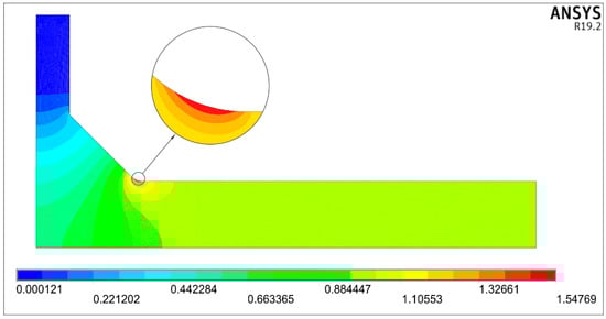
Figure 6.
Heat flux q distribution, interpreted as shearing stress τ for τs = 1 MPa, while θ = 45°, X = 0.25, Y = 0.415 and T/t = 1.
The maximum temperature corresponding to the unit nominal heat flux applied along the right end of the body was equal to 7.089 K. This temperature value resulted from the numerical solution of the boundary-value problem with mixed boundary conditions and was not directly applied over the right edge as a boundary condition.
In subsequent models of T-joints, particular values of X, Y, and θ were systematically changed, while the relative stiffener thickness T/a was constant and equal to one (Z0 = 1). One example of such a set of SCF results for a T-joint subjected to shearing load for θ = 45° is presented in Table 1.

Table 1.
Representation of SCF values for a plate T-joint subjected to shearing load, while θ = 45° and T/a = 1.
Similar 12 sets of SCFs’ data were obtained for other weld angles θ in the range of 30–60° with a step of 2.5°. In this way, 3328 SCF numerical solutions were obtained for each loading mode, which means that 9984 cases of different T-joint shapes had to be modelled and solved for all loading modes.
4. SCF Approximation Formulas
4.1. Numerical and Graphical Representation of P Functions
After normalizing each SCF value with respect to a proper singular term , three approximating functions Pt, Pb, and Ps, corresponding to each loading mode, were determined in the form of polynomials. Their mathematical representation is shown in brackets of Equations (A1)–(A3) given in Appendix A. Graphical representations of these functions, corresponding to the weld angle θ = 45° for three loading modes, are shown in Figure 7, Figure 8 and Figure 9. Numerical values of the exponents n = −0.3264 and ns = −0.2 were obtained from Equations (6) and (7), respectively, for θ = π/4.

Figure 7.
Graphical representation of the function for θ = 45°, n = −0.3264 and Z0 = 1.
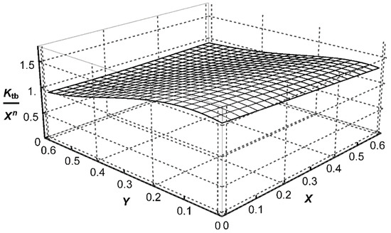
Figure 8.
Graphical representation of the function for θ = 45°, n = −0.3264 and Z0 = 1.
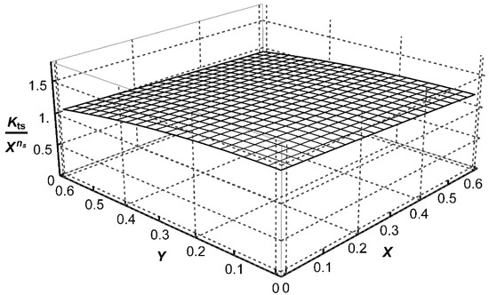
Figure 9.
Graphical representation of the function for θ = 45°, ns = −0.2 and Z0 = 1.
4.2. Validation of the P Functions
Accuracy of the approximating formulas of P functions was verified by comparing calculated SCFs values to their numerical equivalencies obtained using the finite element method. General formula, expressed by Equation (4), is now reduced to Equation (11).
where Z = Z0 = 1 and κ = 1 in the present case. Three examples of such comparisons are presented in Table 2, Table 3 and Table 4 for T-joints subjected to tensile, bending, and shearing loads, respectively, for θ = 45°.
Table 2.
Comparison of Ktt values calculated using Equation (A1) (*) to the corresponding FEM results for various X and Y, while θ = 45° and T/a = 1.
Table 3.
Comparison of Ktb values calculated using Equation (A2) (*) to the corresponding FEM results for various X and Y, while T/a = 1 and θ = 45°.
Table 4.
Comparison of Kts values calculated using Equation (A3) (*) to the corresponding FEM results for various X and Y, while T/a = 1 and θ = 45°.
Similar comparisons were made for various weld angles θ in the range of 30–60°. The maximum percentage error of the approximation was lower than 2%.
4.3. Determination of the Correction Functions κ
Additional FEM modelling was carried out in order to determine the influence of the relative attachment plate thickness Z = T/a on SCF, represented mathematically by a correction function κ. Several thousand new cases of a T-joint were modelled and solved for each loading mode and various proportions of T/a in the range of 1 ≤ T/a ≤ 4.
The general mathematical representation of the correction functions κ in the form of Equation (12).
was derived, which is similar to the one performed by the authors in Reference [30] for cruciform welded joints. Particular values of the exponents, m and p, and coefficients B1-B4, were determined for each loading mode using the least squares method. The best fitting of the functions κt, κb and κs, to the numerical FEM SCF results were obtained for m = 1, for tensile and bending load, and for m = 2 for shearing load, and for p equal to 2.4, 2.6, and 2.0 for tensile, bending, and shearing loads, respectively. Unfortunately, the coefficients Bi depended also on the weld angle θ. Therefore, additional approximations for Bi = fi(θ) were necessary. Mathematical representations of the correction functions κt, κb, and κs, suitable for each loading mode, are given in Appendix A. Some examples of the correction functions κt, κb, and κs for tensile, bending, and shearing loads, respectively, are shown in Figure 10, Figure 11 and Figure 12, for arbitrarily chosen parameters: θ = 45° and T/a equal to 2 and 4.
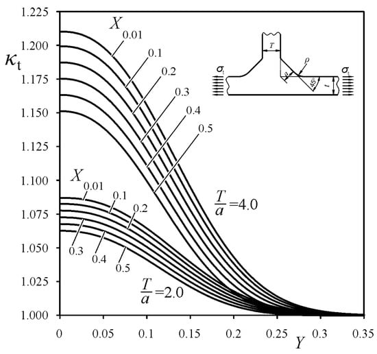
Figure 10.
Correction function κt for tensile load, while θ = 45°.
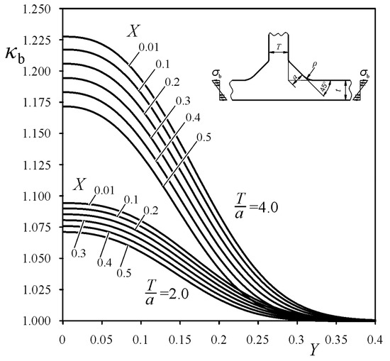
Figure 11.
Correction function κb for the bending load while θ = 45°.
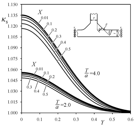
Figure 12.
Correction function κs for the shearing load while θ = 45°.
4.4. Validation of SCF Approximation Functions
Accuracy of the SCF approximation functions, given by the Formulas (A1)–(A3), containing correction functions κt, κb, and κs, > 1, was verified for all loading modes and for the weld angle θ varying in the range of 30–60°. Some examples of the validation are presented in Table 5, Table 6 and Table 7 for arbitrarily chosen angles θ equal to 30°, 45°, and 55°.
Table 5.
Comparison of SCF’s values calculated using Equations (A1)–(A3) (*) to the corresponding FEM results for various T/a ratios, while θ = 30°.
Table 6.
Comparison of SCF’s values calculated using Equations (A1)–(A3) (*) to the corresponding FEM results for various T/a ratios, while θ = 45°.
Table 7.
Comparison of SCF’s values calculated using Equations (A1)–(A3) (*) to the corresponding FEM results for various T/a ratios, while θ = 55°.
Similar validation was made for other weld angles θ with a step of 2.5°. The maximum percentage error found for all analysed cases was lower than 2% with respect to the SCFs’ results obtained numerically using the FEM. Due to the fact that the weld angle θ = 45° is commonly used in engineering applications of such T-joints, extended parametric Equations (A1)–(A3) given in Appendix A, were reduced to Equations (A4)–(A6) presented in Appendix B.
5. Discussion
Several thousand SCF solutions obtained using the FEM as well as corresponding parametric Equations (A1)–(A3) of high accuracy and a wide range of validity, made it possible to draw some more general conclusions regarding the influence of particular geometrical parameters on SCF. The general rule is that particular characteristic geometrical details of the joint located closer to the reference point of the maximum stress σ1max affect this value more significantly than others. In order to explain this phenomenon more precisely, three qualitatively different geometrical cases of a T-joint are shown in Figure 13. Additionally, some alternative, parametric SCF formulas available in the literature [13,15,16,17,19] and related to T-joints are also given in Appendix C.
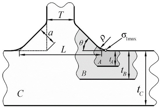
Figure 13.
Characteristic dimensional proportions representing the influence of characteristic geometrical dimensions on SCF.
In case A, shown in Figure 13, the main plate is relatively thin compared to other dimensions of the joint, tA << L, while the magnitude of the weld toe radius ρ is of the same order as the plate thickness tA. In such a case, SCF values depend mainly on the tA/ρ ratio. For example, when tA/ρ changes in the range of 0.8–5.0, Ktt varies from 1.16 to 1.63 and does not depend on the weld angle θ in the range of 30–60°. Similar behaviour is observed for tA/ρ in the range of 0.8–4.0, where Ktb varies from 1.16 to 1.66. In case B, when the weld toe radius ρ is much smaller than in the previous case and L >> tB, SCF values should depend on the quantities tB/ρ and θ.
Equations (A9) and (A12) presented in Appendix C and numerical SCF data shown in Table 8 confirm such a conclusion.
Table 8.
Influence of the weld angle θ and t/ρ ratio on SCF for L > 4t.
However, accuracy of the formulas given in Appendix C depends on the mathematical representation chosen by the authors, assumed range of validity, and the accuracy of data used in approximations. Some comparisons of SCFs obtained from various equations to the FEM results carried out in the present work are shown in Table 9 and Table 10 for θ = 45°.
Table 9.
Accuracy of Equations (A1) and (A7)–(A10) for a T-joint subjected to tension, where: θ = 45°, h = hp, t = T, h/t = 0.75, 0.025 ≤ ρ/t ≤ 0.35, #—out of range.
Table 10.
Accuracy of Equations (A2) and (A11)–(A14) for the T-joint subjected to bending, where: θ = 45°, h = hp, t = T, h/t = 0.75, 0.025 ≤ ρ/t ≤ 0.35, #—out of range.
In case C, shown in Figure 13, mutual relations between L and tC become important, especially when the L is much shorter than tC. The presence of such a quantity, L/tC, can be observed directly in Equations (A10) and (A14). In a general case, such an influencing parameter depends on the thickness of the stiffener, T, leg lengths, weld angle θ, and the weld toe radius ρ. Therefore, it seems reasonable to use all these quantities in order to derive “effective length” of the joint and, as a consequence, reach better SCF approximations than by a simple use of L. It is also worth noting that SCFs used in Equations (A10) and (A14) are defined in a different manner than in other formulas presented in this work. They are related to the maximum longitudinal stress component at the weld toe and not to the maximum principal stress σ1max. Therefore, SCF values obtained from Equations (A10) and (A14) and shown in Table 9 and Table 10, are a few percent underestimated compared with appropriate FEM results.
Particular data given in Table 9 and Table 10 represent only some comparative examples of SCF values with respect to the FEM results. Therefore, these results cannot be generalised to assess accuracy of each formula. Some of these results denoted by (#) mean that they formally lie out of range of validity assumed by the authors. However, in many cases, the accuracy remains satisfactory.
It may be assumed that the range of validity of the formulas (A8) and (A13), proposed by Tsuji [17], is similar to that for Equations (A7) and (A11) reported by Ushirokawa and Nakayama [16].
6. Conclusions
Systematic numerical FEM modelling including more than 22,600 cases of welded plate T-joints made it possible to derive three approximating SCF’s formulas for axial, bending, and shearing loads. Five geometrical parameters: ρ, a, θ, t, and T were considered as independent variables varying in relatively wide ranges 0 < ρ/a ≤ 1.3, 0 < a/t ≤ 1.3, 1 ≤ T/a ≤ 4, and 30° ≤ θ ≤ 60° covering dimensional proportions of welded plate T-joints used in engineering applications. Two limiting cases are also included in the solutions—when the weld toe radius tends to zero and when the main plate thickness becomes infinite. The accuracy of the formulas is better than 98% compared with numerical FEM results. The use of the proper exponents, n and ns, corresponding to the stress field singularities of a sharp corner dependent on the angle θ, was the key condition in obtaining such an accuracy and range of validity of proposed parametric equations. In the cases of shearing loads, a plane FEM model based on thermal analogy was successfully used.
In spite of the fact that SCF alone is not sufficient for calculating fatigue strength of a structural element, all the parametric formulas given in a closed form may be used as a part of computer-aided procedures for the fatigue strength assessment of welded plate T-joints.
Presented solutions may be applied as a tool for a computer aided assessment in fatigue design of welded plate T-joints. Particularly in:
- (a)
- comparative studies of stress concentration in various geometrical forms of welded T-joints, including the use of fictitious values of the weld toe radii,
- (b)
- hot spot method applied in fatigue design of such joints,
- (c)
- weight function method used in fracture mechanics models for crack initiated at the weld toe,
- (d)
- dealing with the necessity of additional mechanical improvements in the weld toe region.
Author Contributions
Conceptualization, K.L.M. Methodology, K.L.M. Software, P.T. Validation, K.L.M. and P.T. Formal analysis, K.L.M. and P.T. Investigation, K.L.M. and P.T. Resources, K.L.M. and P.T. Data curation, P.T. Writing—original draft preparation, K.L.M. Writing—review and editing, K.L.M. and P.T. Visualization, K.L.M. and P.T. Supervision, K.L.M. Project administration, P.T. Funding acquisition, K.L.M. and P.T. All authors have read and agreed to the published version of the manuscript.
Funding
This publication was financed through the program of the Ministry of Science and Higher Education of Poland named “Regional Initiative of Excellence” in 2019–2022 project number 011/RID/2018/19.
Institutional Review Board Statement
Not applicable.
Informed Consent Statement
Not applicable.
Data Availability Statement
Data is contained within the article.
Acknowledgments
This research was co-founded through a subsidy of the Ministry of Science and Higher Education for the discipline of mechanical engineering at the Faculty of Mechanical Engineering, Bialystok University of Technology, project no. WZ/WM-IIM/4/2020.
Conflicts of Interest
The authors declare no conflict of interest.
Nomenclature
| a | theoretical weld throat thickness |
| G | shear modulus |
| h, hp | leg lengths defining the weld size |
| k | thermal conductivity |
| Kt | stress concentration factor (SCF) |
| Ktt | stress concentration factor for tensile (axial) load |
| Ktb | stress concentration factor for bending load |
| Kts | stress concentration factor for shearing load |
| m, p | exponents dependent on the loading mode |
| n | stress field exponent for a sharp corner for axial and bending load |
| ns | stress field exponent for a sharp corner subjected to shearing load |
| P | regular function represented by polynomials |
| Pt, Pb, Ps | functions P corresponding to tensile, bending, and shearing load, respectively |
| q | magnitude of the heat flux |
| qmax | magnitude of the maximum heat flux |
| qnom | magnitude of the nominal heat flux at the end of the body |
| t | thickness of the main plate |
| T | thickness of the attachment plate |
| Ttemp | temperature |
| W | displacement component corresponding to the anti–plane shear |
| X = ρ/(ρ + a) | normalized toe radius parameter |
| Y = a/(a + t) | normalized weld thickness parameter |
| Z = T/a | normalized attachment plate thickness parameter |
| Z0 | arbitrarily chosen reference T/a value |
| |∇Ψ| | magnitude of the displacement (temperature) gradient |
| |∇Ψ|max | magnitude of the maximum displacement (temperature) gradient |
| |∇Ψ|nom | magnitude of the nominal displacement (temperature) gradient |
| θ | weld angle |
| κ | correction function for the relative attachment plate thickness T/a |
| κt | correction function κ for tensile (axial) load |
| κb | correction function κ for bending load |
| κs | correction function κ for shearing load |
| Ψ(x,y) | potential function representing temperature or anti–plane displacement |
| ∂Ψ/∂n | normal derivative at the bounding contour |
| ρ | weld toe radius |
| σ1 | first principal stress produced by normal or bending load |
| σ1max | maximum value of the first principal stress at the weld toe zone |
| σt | nominal tensile (axial) stress |
| σb | nominal bending stress |
| τmax | maximum shear stress at the weld toe due to shearing load |
| τs | nominal shear stress |
Appendix A
Approximating SCFs’ Formulas for a Welded Plate T-Joint Subjected to Axial, Bending, and Shearing Loads
Independent variables: ρ, a, θ, t, T;
Normalized quantities: X = ρ/(ρ + a), Y = a/(a + t); Z = T/a;
Range of validity: 0 < ρ/a ≤ 1.3; 0 < a/t ≤ 1.3; 1 ≤ T/a ≤ 4; 30° ≤ θ ≤ 60°.
In all formulas, θ is expressed in radians.
Exponent of the singular term for:
Axial and bending load:
Shearing load:
Accuracy: maximum percentage error lower than 2% compared to the FEM results
Tensile (axial) load:
where:
Bending load:
where:
Shearing load:
where:
Appendix B
Parametric Formulas for Calculating SCFs, while θ = 45°
Tensile (axial) load:
where:
Bending load:
where:
Shearing load:
where:
Appendix C
Alternative Parametric Formulas for Calculating SCF for Plate T-Joints Subjected to Tensile and Bending Loads
Plate T-joint—axial load
Ushirokawa and Nakayama (1983). Range of validity: 0.025 ≤ ρ/t ≤ 0.35, 20° ≤ θ ≤ 50°, T/t = 1, hp/t = 0.75.
Tsuji (1990): range of validity not precisely defined.
Monahan (1995), range of validity: 0.02 ≤ ρ/t ≤ 0.066, 30° ≤ θ≤60°, L/t = 2.8.
Brennan et al. (2000), range of validity: 0.01 ≤ ρ/t ≤ 0.066, 30° ≤ θ≤60°, 0.3 ≤ L/t ≤ 4.0
Plate T-joint—bending load
Ushirokawa and Nakayama (1983), range of validity: 0.025 ≤ ρ/t ≤ 0.35, 20° ≤ θ≤50°, T/t = 1, hp/t = 0.75.
Niu and Glinka (1987), range of validity: 0.02 ≤ ρ/t ≤ 0.066, 30° ≤ θ≤60°, T/t = 1, h/t = 1.
Tsuji (1990), range of validity not precisely defined.
Brennan et al. (2000), range of validity: 0.01 ≤ ρ/t ≤ 0.066, 30° ≤ θ≤60°, 0.3 ≤ L/t ≤ 4.0.
References
- Gurney, T.R. Fatigue of Welded Structures, 2nd ed.; Cambridge University Press: Cambridge, UK, 1979. [Google Scholar]
- European Committee for Standardization (CES). EN 1993-1-9:2005 Eurocode 3: Design of Steel Structures—Part. 1–9: Fatigue; CES: Brussels, Belgium, 2005. [Google Scholar]
- Hobbacher, A.F. The new IIW recommendations for fatigue assessment of welded joints and components—A comprehensive code recently updated. Int. J. Fatigue 2009, 31, 50–58. [Google Scholar] [CrossRef]
- Fricke, W. IIW Recommendations for the Fatigue Assessment of Welded Structures by Notch Stress Analysis; Woodhead Publishing: Cambridge, UK, 2012; pp. 2–41. [Google Scholar]
- Kranz, B.; Sonsino, C.M. Verification of FAT Values for the Application of the Notch Stress Concept with the Reference Radii Rref = 1.00 and 0.05 mm. Weld. World 2010, 54, R218–R224. [Google Scholar] [CrossRef]
- Fricke, W. IIW guideline for the assessment of weld root fatigue. Weld. World 2013, 57, 753–791. [Google Scholar] [CrossRef]
- International Standard Organization (ISO). EN ISO 9692-1:2013 Welding and Allied Processes—Types of Joint Preparation—Part. 1: Manual Metal. Arc Welding, Gas.-Shielded Metal. Arc Welding, Gas. Welding, TIG Welding and Beam Welding of Steels; International Organization for Standardization: Geneva, Switzerland, 2013. [Google Scholar]
- Zhao, X.L.; Packer, J.A. Fatigue Design Procedure for Welded Hollow Section Joints, 1st ed.; Abington Publishing: Nashville, TN, USA, 2000. [Google Scholar]
- Mashiri, R.; Zhao, X.L.; Grundy, P. Stress concentration factors and fatigue failure of welded T-connections in circular hollow sections under in-plane bending. Int. J. Struct. Stab. Dyn. 2004, 4, 403–422. [Google Scholar] [CrossRef]
- Kršćanski, S.; Turkalj, G. FEM stress concentration factors for fillet welded CHS-plate T-joint. Eng. Rev. 2012, 32, 147–155. [Google Scholar]
- Saini, D.S.; Karmakar, D.; Ray-Chaudhuri, S. A review of stress concentration factors in tubular and non-tubular joints for design of offshore installations. JOES 2016, 1, 186–202. [Google Scholar] [CrossRef]
- Carpinteri, A.; Boaretto, J.; Fortese, G.; Giordani, F.; Iturrioz, I.; Ronchei, C.; Scorza, D.; Vantadori, S. Fatigue life estimation of fillet-welded tubular T-joints subjected to multiaxial loading. Int. J. Fatigue 2017, 101, 263–270. [Google Scholar] [CrossRef]
- Niu, X.; Glinka, G. The weld profile effect on stress intensity factors in weldments. Int J. Fract. 1987, 35, 3–20. [Google Scholar]
- Bhuyan, G.; Vosikovsky, O. Prediction of fatigue crack initiation lives for welded plate T-joints based on the local stress-strain approach. Int. J. Fatigue 1989, 11, 153–159. [Google Scholar] [CrossRef]
- Monahan, C.C. Early Fatigue Crack Growth at Welds; WIT PRESS/Computational Mechanics Publications: Southampton, UK, 1995. [Google Scholar]
- Ushirokawa, O.; Nakayama, E. Stress concentration factor at welded joints. Ishikawajima Harima Eng. Rev. 1983, 23, 351–355. [Google Scholar]
- Tsuji, I. Estimation of stress concentration factor at weld toe of non-load carrying fillet welded joints. Trans. West. Jpn. Soc. Nav. Archit. 1990, 80, 241–251. [Google Scholar]
- Iida, K.; Uemura, T. Stress concentration factor formulas widely used in Japan. Fatigue Fract. Eng. Mater. Struct. 1996, 19, 779–786. [Google Scholar] [CrossRef]
- Brennan, F.P.; Peletiesa, P.; Hellierb, A.K. Predicting weld toe stress concentration factors for T and skewed T-joint plate connections. Int. J. Fatigue 2000, 22, 573–584. [Google Scholar] [CrossRef]
- Dabiri, M.; Ghafouri, M.; Raftar, H.R.R.; Björk, T. Neural network-based assessment of the stress concentration factor in a T-welded joint. J. Constr. Steel Res. 2017, 128, 567–578. [Google Scholar] [CrossRef]
- Bell, R.; Vosikovsky, O.; Bain, S.A. The significance of weld toe undercuts in the fatigue of steel plate T-joints. Int. J. Fatigue 1989, 11, 3–11. [Google Scholar] [CrossRef]
- Hou, C.Y. Fatigue analysis of welded joints with the aid of real three-dimensional weld toe geometry. Int. J. Fatigue 2007, 29, 772–785. [Google Scholar] [CrossRef]
- Tarasiuk, P.; Molski, K.L.; Szymaniuk, A. Fatigue designing of welded agricultural wheels. Eksploat. Niezawodn. 2013, 15, 123–128. [Google Scholar]
- Zhao, W.; Hsu, W.-T. Re-Evaluation of Fatigue Thickness Effect Based on Fatigue Test Database. J. Mar. Sci. Eng. 2020, 8, 895. [Google Scholar] [CrossRef]
- Wang, Y.; Luo, Y.; Tsutsumi, S. Parametric Formula for Stress Concentration Factor of Fillet Weld Joints with Spline Bead Profile. Materials 2020, 13, 4639. [Google Scholar] [CrossRef]
- Terán, G.; Albiter, A.; Cuamatzi-Meléndez, R. Parametric evaluation of the stress concentration factors in T-butt welded connections. Eng. Struct. 2013, 56, 1484–1495. [Google Scholar] [CrossRef]
- Costa, J.D.M.; Jesus, J.S.; Loureiro, A.; Ferreira, J.A.M.; Borrego, L.P. Fatigue life improvement of mig welded aluminium T-joints by friction stir processing. Int. J. Fatigue 2014, 61, 244–254. [Google Scholar] [CrossRef]
- Luo, Y.; Ma, R.; Tsutsumi, S. Parametric formulae for elastic stress concentration factor at the weld toe of distorted butt-welded joints. Materials 2020, 13, 169. [Google Scholar] [CrossRef] [PubMed]
- Stenberg, T.; Barsoum, Z.; Hedlund, J.; Josefsson, J. Development of a computational fatigue model for evaluation of weld quality. Weld. World 2019, 63, 1771–1785. [Google Scholar] [CrossRef]
- Haagensen, P.J.; Maddox, S.J. Recommendations on Methods for Improving the Fatigue Strength of Welded Joints; Woodhead Publishing: Cambridge, UK, 2013; ISBN 9781782420644. [Google Scholar]
- Molski, K.L.; Tarasiuk, P.; Glinka, G. Stress concentration at cruciform welded joints under axial and bending loading modes. Weld. World 2020, 64, 1867–1876. [Google Scholar] [CrossRef]
- Molski, K.L.; Tarasiuk, P. Stress Concentration Factors for Butt-Welded Plates Subjected to Tensile, Bending and Shearing Loads. Materials 2020, 13, 1798. [Google Scholar] [CrossRef]
- Seweryn, A.; Molski, K.L. Elastic stress singularities and corresponding generalized stress intensity factors for angular corners under various boundary conditions. Eng. Fract. Mech. 1996, 55, 529–556. [Google Scholar] [CrossRef]
Publisher’s Note: MDPI stays neutral with regard to jurisdictional claims in published maps and institutional affiliations. |
© 2021 by the authors. Licensee MDPI, Basel, Switzerland. This article is an open access article distributed under the terms and conditions of the Creative Commons Attribution (CC BY) license (http://creativecommons.org/licenses/by/4.0/).