
Reliability Analysis for Unrepairable Automotive Components

 ,
,  , , , ,
Abstract
1. Introduction
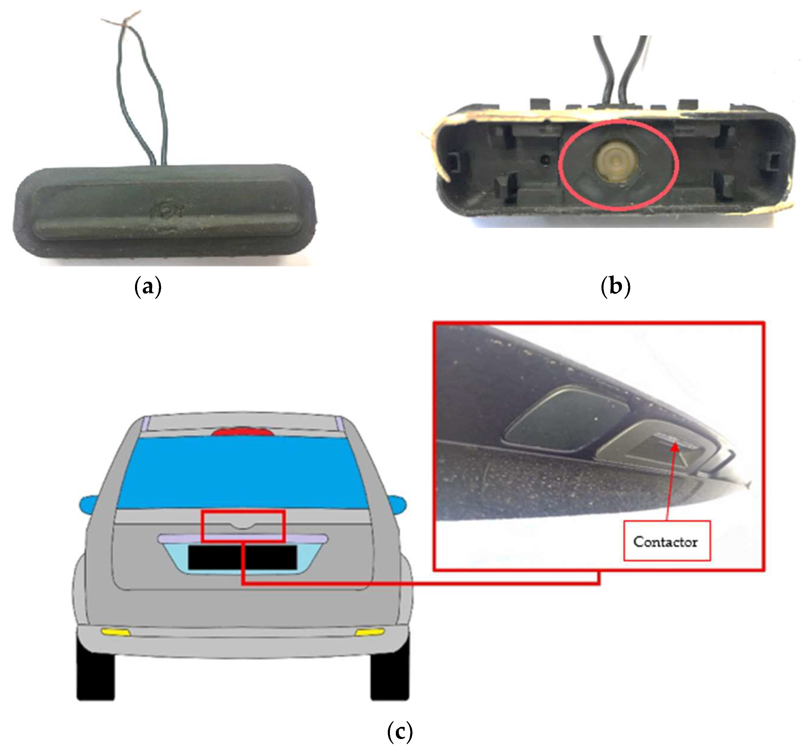
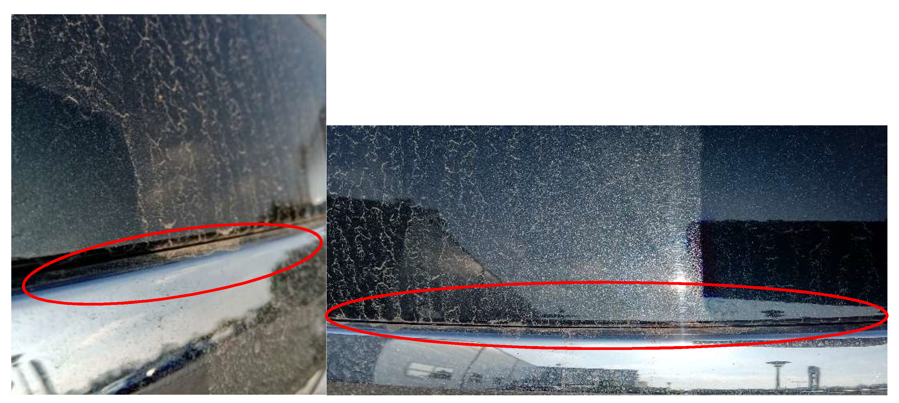
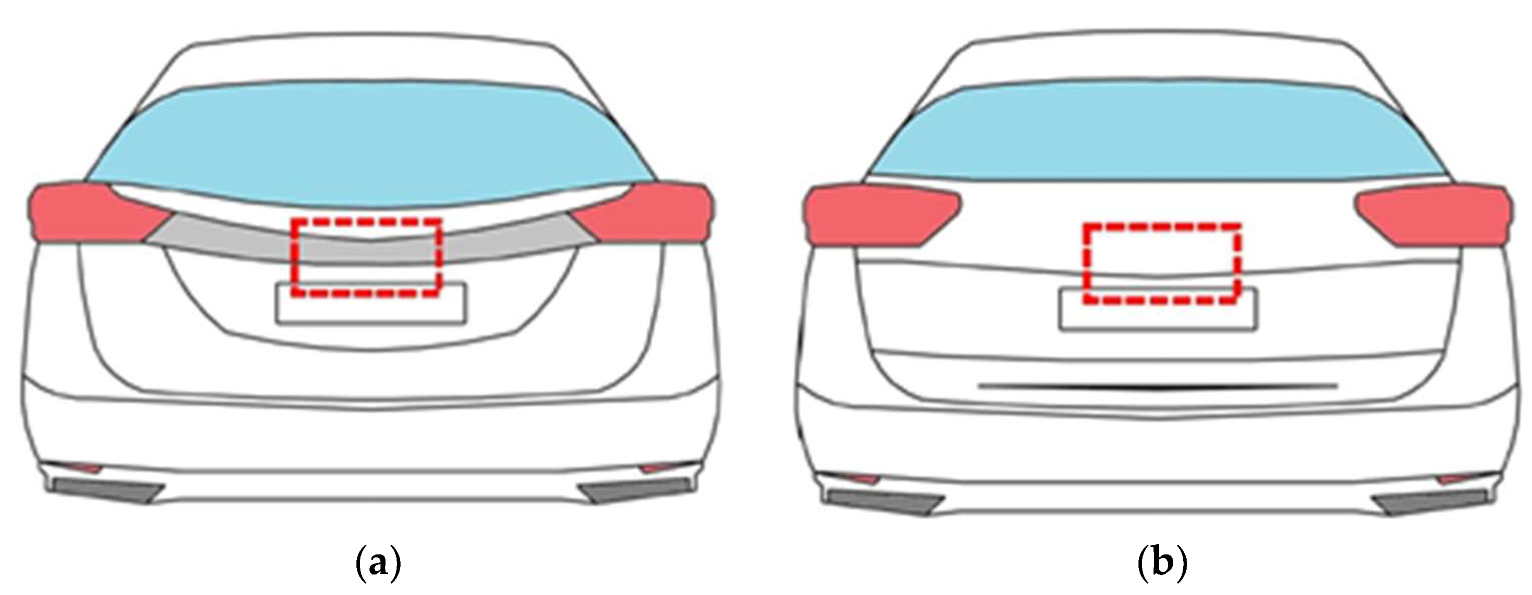
2. Subject of Research
3. Failure Data and Probability Distribution Fitting
- -
- H0: the distribution represents the data,
- -
- H1: the distribution does not represent the data.
4. Results Analysis
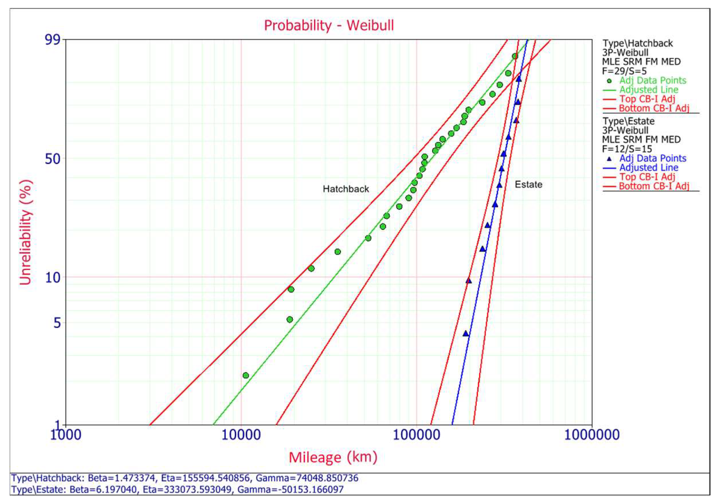
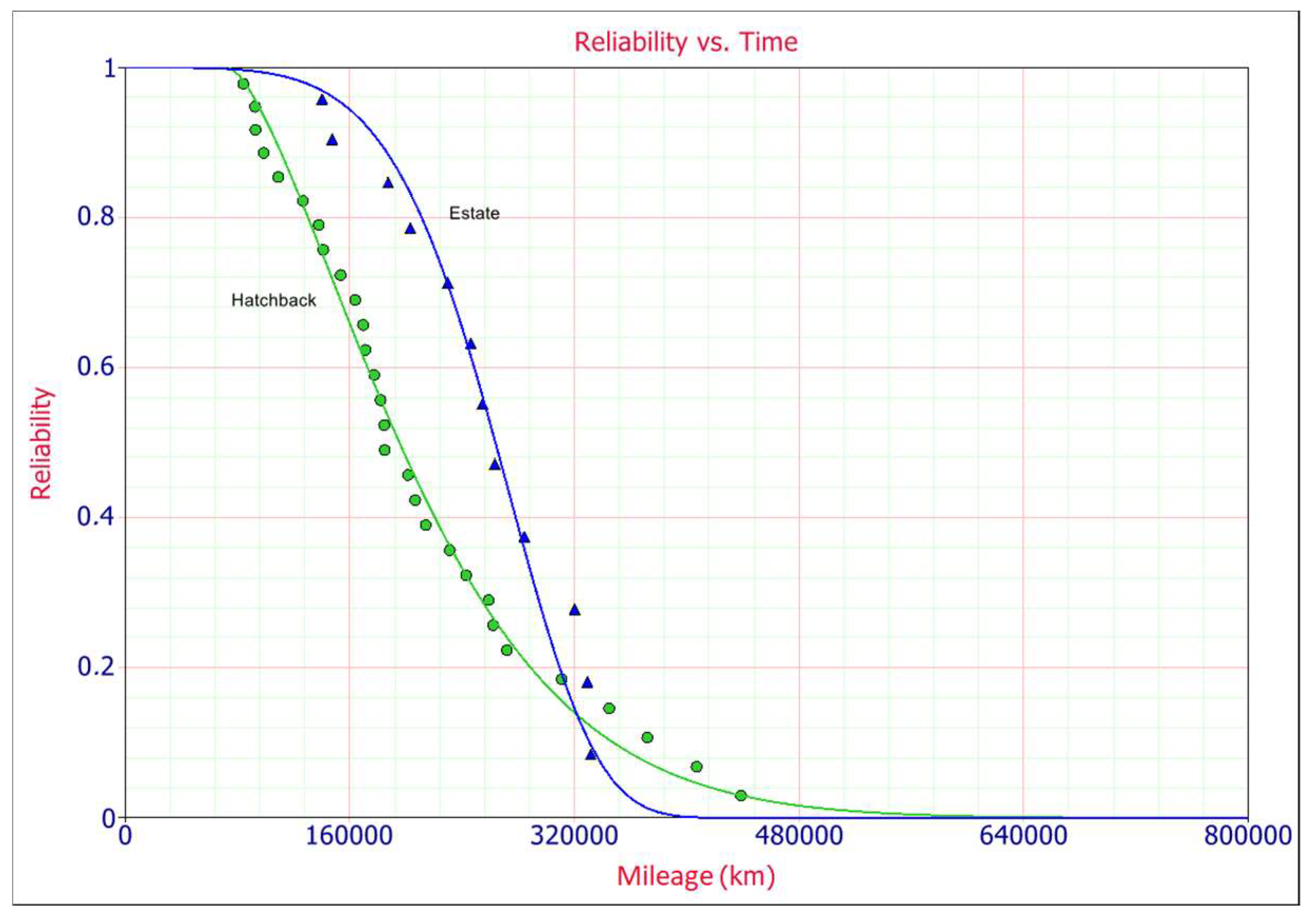
4.1. Data Interpretation
4.2. Optimal Maintenance Strategy
4.3. The Method of Solving the Problem
5. Conclusions
Author Contributions
Funding
Institutional Review Board Statement
Informed Consent Statement
Data Availability Statement
Conflicts of Interest
References
- Lewis, M. Designing reliability-durability testing for automotive electronics—A commonsense approach. In Proceedings of the 46th Annual Technical Meeting-Institute of Environmental Sciences and Technology, Providence, RI, USA, 30 April–4 May 2000; Volume 46, pp. 175–179. [Google Scholar]
- Krolo, A.; Bertsche, B. An approach for the advanced planning of a reliability demonstration test based on a Bayes procedure. In Proceedings of the Annual Reliability and Maintainability Symposium Conference, Tampa, FL, USA, 27–30 January 2003; pp. 288–294. [Google Scholar]
- Kleyner, A. Reliability demonstration in product validation testing. In Handbook of Performability Engineering; Misra, K.B., Ed.; Springer: London, UK, 2008. [Google Scholar] [CrossRef]
- Ascher, H.; Feingold, H. Repairable Systems Reliability—Modeling, Inference, Misconceptions, and Their Causes; Marcel. Dekker: New York, NY, USA, 1984. [Google Scholar]
- Elmahdy, E.E. Modelling reliability data with finite weibull or lognormal mixture distributions. Appl. Math. Inf. Sci. 2017, 11, 1081–1089. [Google Scholar] [CrossRef]
- Patra, A.P.; Söderholm, P.; Kumar, U. Uncertainty estimation in railway track lifecycle cost: A case study from Swedish national Rail Administration. Proc. Inst. Mech. Eng. Part F J. Rail Rapid Transit 2009, 223, 285–293. [Google Scholar] [CrossRef]
- Lewis, E.E. Introduction to Reliability Engineering, 2nd ed.; McGraw-Hill: New York, NY, USA, 1994. [Google Scholar]
- Przystupa, K. Reliability assessment method of device under incomplete observation of failure. In Proceedings of the 18th International Conference on Mechatronics-Mechatronika (ME), Brno, Czech Republic, 5–7 December 2018; pp. 1–6. [Google Scholar]
- Power Law Model-Goodness of Fit Tests and Estimation Methods; IEC 61710; IEC Standards: Geneva, Switzerland, 2013.
- Kozieł, J.; Przystupa, K. Using the FTA method to analyse the quality of an uninterruptible power supply unitreparation UPS. Przegląd Elektrotechniczny 2019, 95, 77–80. [Google Scholar]
- Lawless, J.F. Statistical Models and Methods for Lifetime Data; John Wiley & Sons, Inc.: New York, NY, USA, 1982. [Google Scholar]
- Fuc, P.; Rymaniak, L.; Ziolkowski, A. The correlation of distribution of PM number emitted under actual conditions of operation by PC and HDV vehicles. In WIT Transactions on Ecology and the Environment; WIT Press: Billerica, MA, USA, 2013; Volume 174, pp. 207–2019. ISBN 978-1-84564-718-6. [Google Scholar]
- Gill, A. Optimisation of the technical object maintenance system taking account of risk analysis results. Maint. Reliab. 2017, 19, 420–431. [Google Scholar] [CrossRef]
- Hajkowski, J.; Popielarski, P.; Sika, R. Prediction of HPDC casting properties made of AlSi9Cu3 alloy. In Advances in Manufacturing; Springer: Cham, Germany, 2017; pp. 621–631. [Google Scholar] [CrossRef]
- Dolce, J.E. Analytical Fleet Maintenance Management; SAE International: Warrendale, PA, USA, 1994. [Google Scholar]
- Młyńczak, M. Analiza Danych Eksploatacyjnych w Badaniach Niezawodności Obiektów Technicznych. Zesz. Nauk. Wyższej Szkoły Oficer. Wojsk Lądowych Im. Gen. T. Kościuszki 2011, 1, 159, 177–184. Available online: http://yadda.icm.edu.pl/baztech/element/bwmeta1.element.baztech-article-BATA-0010-0015 (accessed on 1 September 2021).
- Trojanowska, J.; Dostatni, E. Application of the theory of constraints for project management. Manag. Prod. Eng. Rev. 2017, 8, 87–95. [Google Scholar] [CrossRef]
- Żurek, J.; Ziółkowski, J. Method of formulating the required number of vehicles for delivery aircrafts in aviation fuel. J. KONBiN 2017, 44, 347–358. [Google Scholar] [CrossRef][Green Version]
- Rogalewicz, M.; Sika, R.; Popielarski, P.; Wytyk, G. Forecasting of steel consumption with use of nearest neighbours method. In Proceedings of the MATEC Web of Conferences, Malacca, Malaysia, 25–27 February 2017. [Google Scholar] [CrossRef][Green Version]
- Andrzejczak, K.; Młyńczak, M.; Selech, J. Computerization of operation process in municipal transport. In Contemporary Complex Systems and Their Dependability; Zamojski, W., Mazurkiewicz, J., Sugier, J., Walkowiak, T., Kacprzyk, J., Eds.; Advances in Intelligent Systems and Computing; Springer: Cham, Germany, 2018; pp. 13–22. [Google Scholar] [CrossRef]
- Andrzejczak, K.; Selech, J. Quantile analysis of the operating costs of the public transport fleet. Transp. Probl. 2017, 12, 103–111. [Google Scholar] [CrossRef]
- Żurek, J.; Ziółkowski, J.; Borucka, A. Application of Markov processes to the method for analysis of combat vehicle operation in the aspect of their availability and readiness, safety and reliability. In Theory and Applications; Cepin, M., Briš, R., Eds.; Taylor & Francis Group: London, UK, 2017; pp. 2343–2352. ISBN 978-1-138-62937-0. [Google Scholar]
- Genschel, U.; Meeker, W.Q. A comparison of maximum likelihood and median rank regression for weibull estimation. In Proceedings of the Joint Statistical Meetings, Salt Lake City, UT, USA, 30 July 2007. [Google Scholar]
- Genschel, U.; Meeker, W.Q. A Comparison of maximum likelihood and median-rank regression for weibull estimation. Qual. Eng. 2010, 22, 236–255. [Google Scholar] [CrossRef]
- Nelson, W. Weibull analysis of reliability data with few or no failures. J. Qual. Technol. 1985, 17, 140–146. [Google Scholar] [CrossRef]
- Gertsbakh, L. Reliability Theory with Applications to Preventive Maintenance; Springer: Cham, Germany, 2000. [Google Scholar]
- Hirose, H. Bias correction for the maximum likelihood estimation in two-parameter weibull distribution. IEEE Trans. Dielectr. Electr. Insul. 1999, 6, 66–68. [Google Scholar] [CrossRef]
- Selech, J.; Andrzejczak, K. An aggregate criterion for selecting a distribution for times to failure of components of rail vehicles. Maint. Reliab. 2020, 22, 102–111. [Google Scholar] [CrossRef]
- Cox, S.; Tait, R. Safety, Reliability and Risk Management: An Integrated Approach, 2nd ed.; Butterworth Heinemann: Oxford, UK, 1998. [Google Scholar]
- Wang, N.; Chang, Y.-C.; El-Sheikh, A.A. Monte Carlo simulation approach to life cycle cost management. Struct. Infrastruct. Eng. 2002, 8, 739–746. [Google Scholar] [CrossRef]
- ReliaSoft Corporation. Life Data (Weibull) Analysis Reference; ReliaSoft Publishing: Tucson, AZ, USA, 2008. [Google Scholar]
- Kececioglu, D. Reliability and Life Testing Handbook; Prentice Hall: Hoboken, NJ, USA, 1993; Volume 1. [Google Scholar]
- Pulido, J. Life data analysis using the competing failure modes technique. In Proceedings of the 2015 Annual Reliability and Maintainability Symposium (RAMS), Palm Harbor, FL, USA, 26–29 January 2015. [Google Scholar] [CrossRef]
- Maintenance, Replacement, and Reliability: Theory and Applications, 2nd ed.; CRC Press: Boca Raton, FL, USA, 2013. [CrossRef]
- Dhillon, B.S. Maintainability, Maintenance and Reliability for Engineers; Taylor & Francis Group, LLC: Boca Raton, FL, USA, 2006. [Google Scholar]
- Frangopol, D.; Tsompanakis, Y. Maintenance and Safety of Aging Infrastructure: Structures and Infrastructures Book Series, 1st ed.; CRC Press: Boca Raton, FL, USA, 2014; Volume 10. [Google Scholar] [CrossRef]


| F/S | Mileage [km] | Car Body Type | F/S | Mileage [km] | Car Body Type | F/S | Mileage [km] | Car Body Type |
|---|---|---|---|---|---|---|---|---|
| F | 52,621 | H | F | 126,639 | E | F | 272,945 | H |
| F | 57,801 | H | F | 128,676 | H | S | 21,147 | E |
| F | 58,001 | H | F | 133,390 | H | S | 21,169 | E |
| F | 61,628 | H | F | 143,159 | E | S | 21,772 | E |
| F | 68,100 | H | F | 144,041 | H | S | 23,071 | E |
| F | 79,051 | H | F | 151,230 | H | S | 27,165 | H |
| F | 85,974 | H | F | 153,345 | E | S | 36,019 | E |
| F | 87,451 | E | F | 158,420 | E | S | 40,208 | E |
| F | 88,050 | H | F | 161,200 | H | S | 44,374 | H |
| F | 92,003 | E | F | 163,141 | H | S | 45,895 | E |
| F | 95,636 | H | F | 163,952 | E | S | 49,990 | E |
| F | 102,178 | H | F | 169,230 | H | S | 63,422 | E |
| F | 105,600 | H | F | 176,965 | E | S | 63,519 | H |
| F | 106,639 | H | F | 193,500 | H | S | 86,527 | H |
| F | 110,558 | H | F | 199,263 | E | S | 99,784 | E |
| F | 113,359 | H | F | 204,898 | E | S | 120,111 | E |
| F | 115,000 | H | F | 206,460 | E | S | 128,523 | E |
| F | 115,210 | H | F | 214,521 | H | S | 142,302 | E |
| F | 116,762 | E | F | 231,403 | H | S | 151,209 | E |
| F | 125,489 | H | F | 253,241 | H | S | 164,287 | E |
| S | 171,356 | H |
| Distribution | (K-S) | (rho) | LKV |
|---|---|---|---|
| 1P-Exponential | 98.6344 | 13.157 | −373.271 |
| 2P-Exponential | 46.7258 | 5.121 | −357.329 |
| Normal | 36.3504 | 5.114 | −360.985 |
| Lognormal | 0.00136 | 2.168 | −357.914 |
| 2P-Weibull | 13.3673 | 3.803 | −359.422 |
| 3P-Weibull | 0.0004 | 2.316 | −356.841 |
| Gamma | 1.6526 | 2.682 | −358.212 |
| G-Gamma | 0.0018 | 2.170 | −357.914 |
| Logistic | 10.3364 | 3.544 | −361.249 |
| Loglogistic | 0.00697 | 2.172 | −358.661 |
| Gumbel | 58.8010 | 7.855 | −366.116 |
| Distribution | (K-S) | (rho) | LKV |
|---|---|---|---|
| 1P-Exponential | 91.569 | 17.371 | −160.982 |
| 2P-Exponential | 95.994 | 20.586 | −151.111 |
| Normal | 0.594 | 4.003 | −146.373 |
| Lognormal | 0.020 | 4.846 | −147.220 |
| 2P-Weibull | 2.379 | 3.807 | −146.021 |
| 3P-Weibull | 2.918 | 3.758 | −146.001 |
| Gamma | 0.016 | 4.626 | −146.840 |
| G-Gamma | 9.291 | 6.338 | −143.857 |
| Logistic | 0.328 | 3.580 | −146.749 |
| Loglogistic | 0.002 | 3.919 | −147.255 |
| Gumbel | 5.040 | 4.615 | −146.121 |
| Distribution | K-S | rho | LKV | WDV | Ranking |
|---|---|---|---|---|---|
| 3P-Weibull | 1 | 4 | 1 | 130 | 1 |
| Lognormal | 2 | 1 | 4 | 290 | 2 |
| G-Gamma | 3 | 2 | 3 | 290 | 2 |
| Loglogistic | 4 | 3 | 6 | 490 | 3 |
| Gamma | 5 | 5 | 5 | 500 | 4 |
| 2P-Exponential | 9 | 9 | 2 | 550 | 5 |
| 2P-Weibull | 7 | 7 | 7 | 700 | 6 |
| Logistic | 6 | 6 | 9 | 750 | 7 |
| Normal | 8 | 8 | 8 | 800 | 8 |
| Gumbel | 10 | 10 | 10 | 1000 | 9 |
| 1P-Exponential | 11 | 11 | 11 | 1100 | 10 |
| Distribution | K-S | rho | LKV | WDV | Ranking |
|---|---|---|---|---|---|
| 3P-Weibull | 7 | 2 | 2 | 400 | 1 |
| 2P-Weibull | 6 | 3 | 3 | 420 | 2 |
| Logistic | 4 | 1 | 6 | 470 | 3 |
| Normal | 5 | 5 | 5 | 500 | 4 |
| Gamma | 2 | 7 | 7 | 500 | 4 |
| G-Gamma | 9 | 9 | 1 | 500 | 4 |
| Loglogistic | 1 | 4 | 9 | 530 | 5 |
| Gumbel | 8 | 6 | 4 | 580 | 6 |
| Lognormal | 3 | 8 | 8 | 600 | 7 |
| 1P-Exponential | 10 | 10 | 11 | 1050 | 8 |
| 2P-Exponential | 11 | 11 | 10 | 1050 | 8 |
| Body Type | Year of Registration | Sum | ||||||
|---|---|---|---|---|---|---|---|---|
| 2009 | 2010 | 2011 | 2012 | 2013 | 2014 | 2015 | ||
| Hatchback | 2402 | 3876 | 2418 | 1705 | 1207 | 1766 | 1597 | 14,971 |
| Estate | 538 | 1379 | 1338 | 1131 | 1084 | 1817 | 1049 | 8336 |
| Type of Body Car | Minimal Replacement Cost [EUR] | Optimal Time Interval [km] | Cost/Per Car [EUR] | Cost for all Cars (2009–2015) [EUR] |
|---|---|---|---|---|
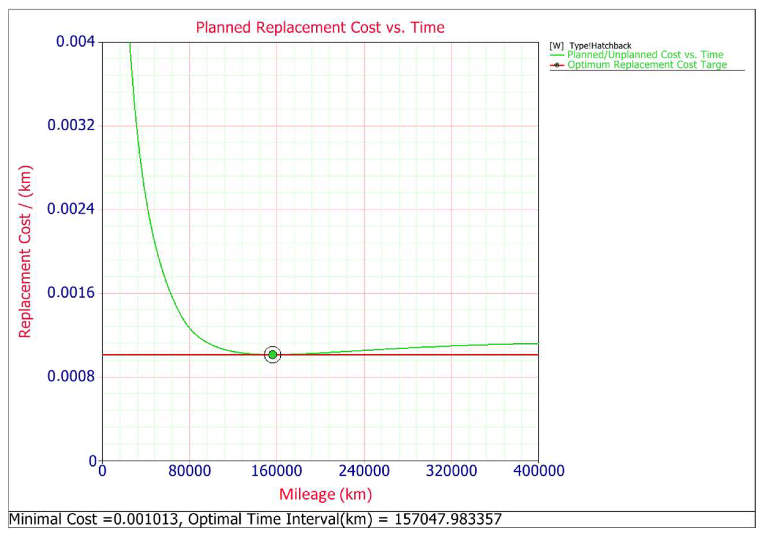
| Hatchback | 0.000223 | 157,047.98 | 35.02 | 349,540 |
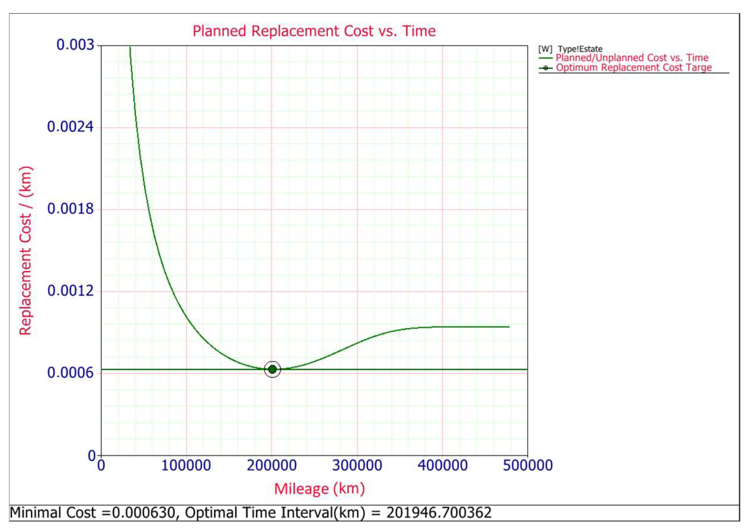
| Estate | 0.000139 | 201,946.70 | 28.07 | 155,998 |
| Total cost | 505,538 |
Publisher’s Note: MDPI stays neutral with regard to jurisdictional claims in published maps and institutional affiliations. |
© 2021 by the authors. Licensee MDPI, Basel, Switzerland. This article is an open access article distributed under the terms and conditions of the Creative Commons Attribution (CC BY) license (https://creativecommons.org/licenses/by/4.0/).
Share and Cite
Ulbrich, D.; Selech, J.; Kowalczyk, J.; Jóźwiak, J.; Durczak, K.; Gil, L.; Pieniak, D.; Paczkowska, M.; Przystupa, K. Reliability Analysis for Unrepairable Automotive Components. Materials 2021, 14, 7014. https://doi.org/10.3390/ma14227014
Ulbrich D, Selech J, Kowalczyk J, Jóźwiak J, Durczak K, Gil L, Pieniak D, Paczkowska M, Przystupa K. Reliability Analysis for Unrepairable Automotive Components. Materials. 2021; 14(22):7014. https://doi.org/10.3390/ma14227014
Chicago/Turabian StyleUlbrich, Dariusz, Jaroslaw Selech, Jakub Kowalczyk, Jakub Jóźwiak, Karol Durczak, Leszek Gil, Daniel Pieniak, Marta Paczkowska, and Krzysztof Przystupa. 2021. "Reliability Analysis for Unrepairable Automotive Components" Materials 14, no. 22: 7014. https://doi.org/10.3390/ma14227014
APA StyleUlbrich, D., Selech, J., Kowalczyk, J., Jóźwiak, J., Durczak, K., Gil, L., Pieniak, D., Paczkowska, M., & Przystupa, K. (2021). Reliability Analysis for Unrepairable Automotive Components. Materials, 14(22), 7014. https://doi.org/10.3390/ma14227014