
Fiber Optic-Based Thermal Integrity Profiling of Drilled Shaft: Inverse Modeling for Spiral Fiber Deployment Strategy


Abstract
:1. Introduction
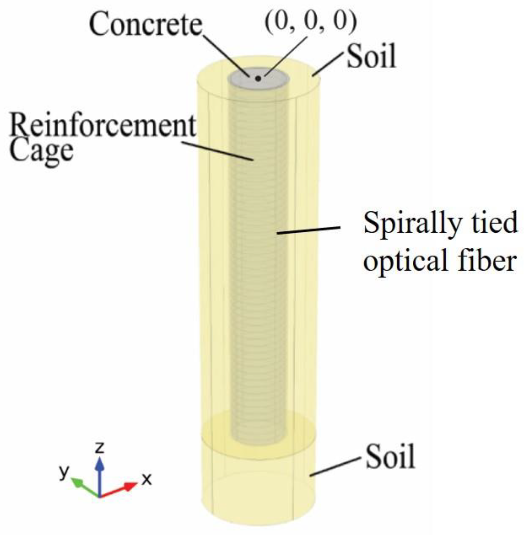
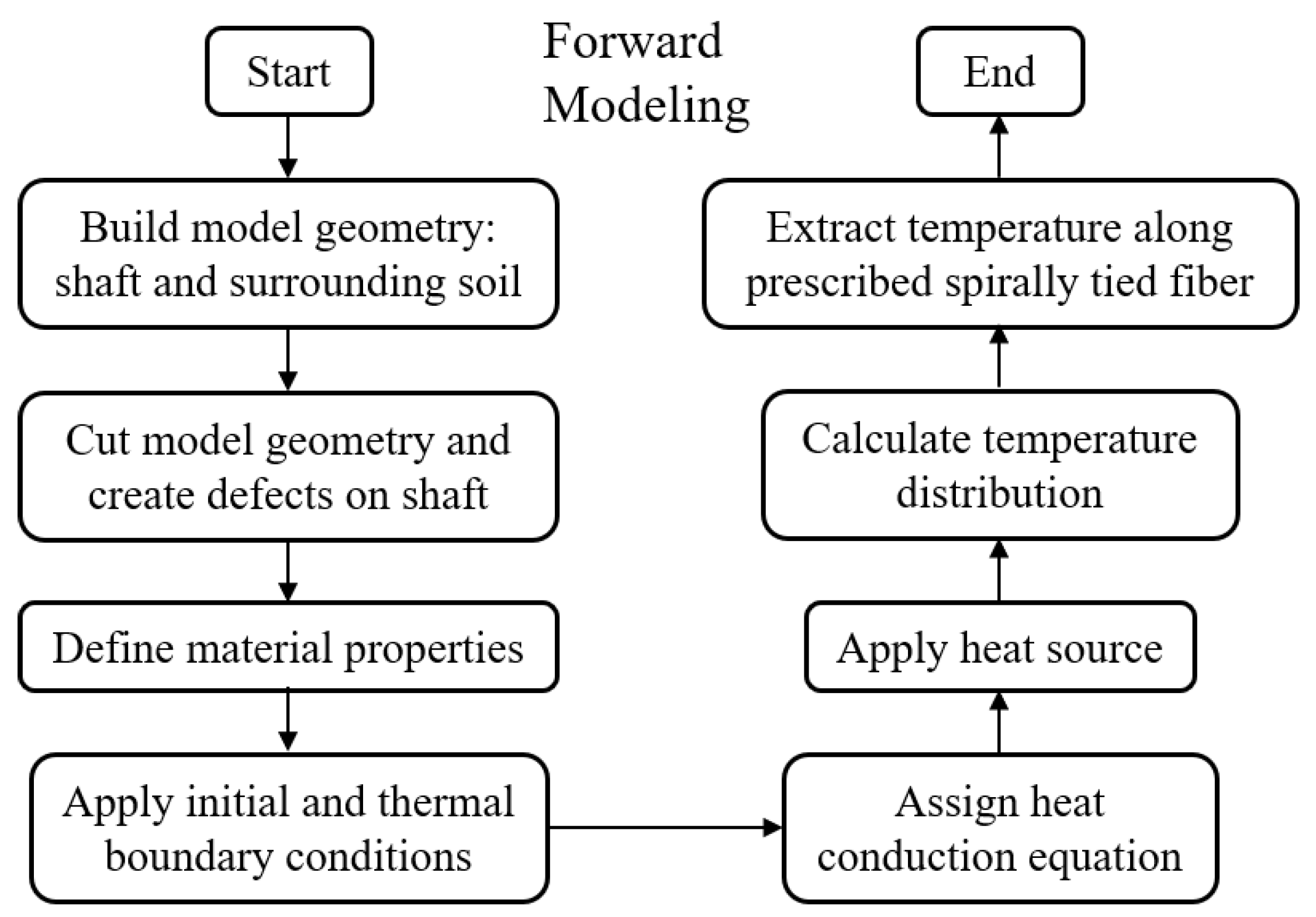
2. Methodology
2.1. Governing Equations
2.2. Heat Production
2.3. Heat Conductivity
2.4. Heat Capacity
2.5. Simulation Parameters
3. Results and Discussion
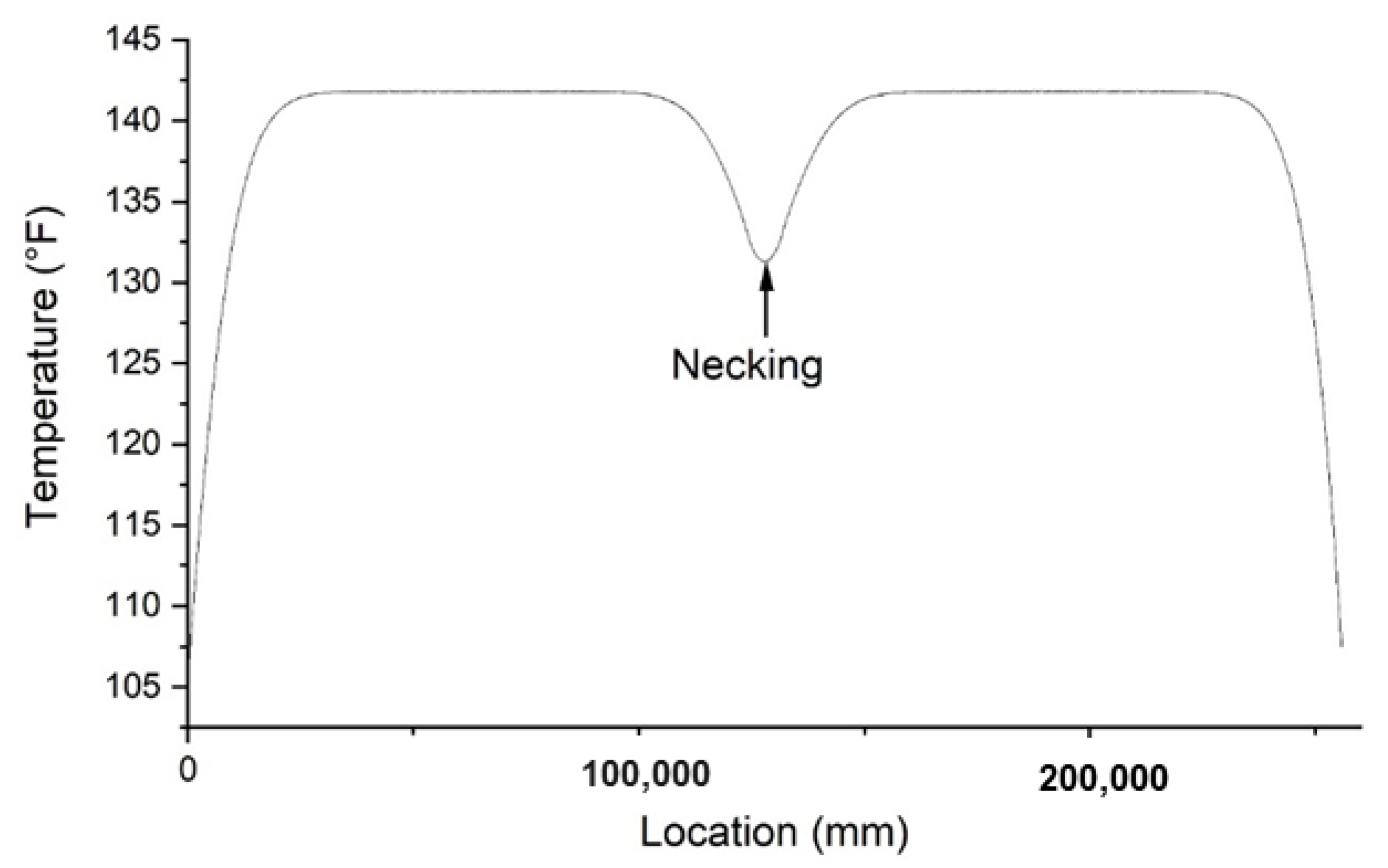
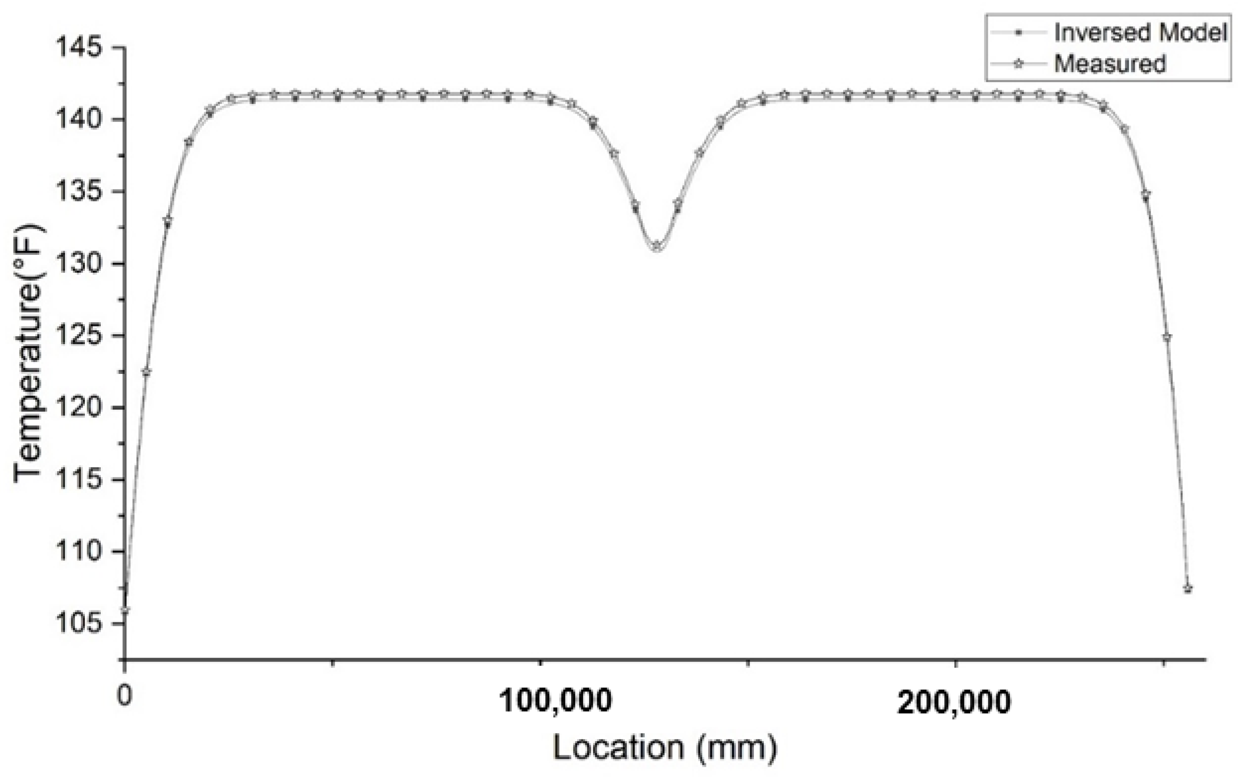
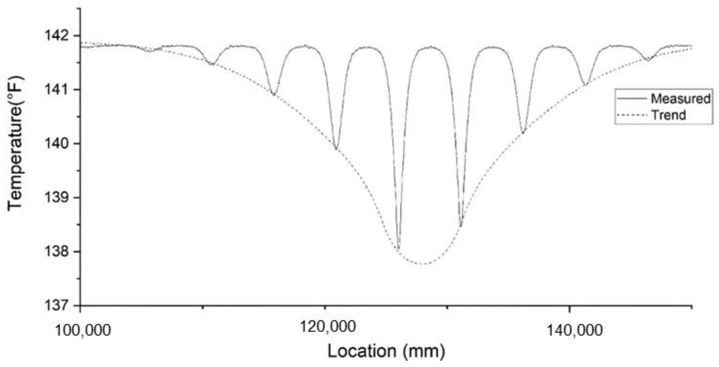
3.1. Necking Defect
3.1.1. Forward Modeling
3.1.2. Inverse Modeling
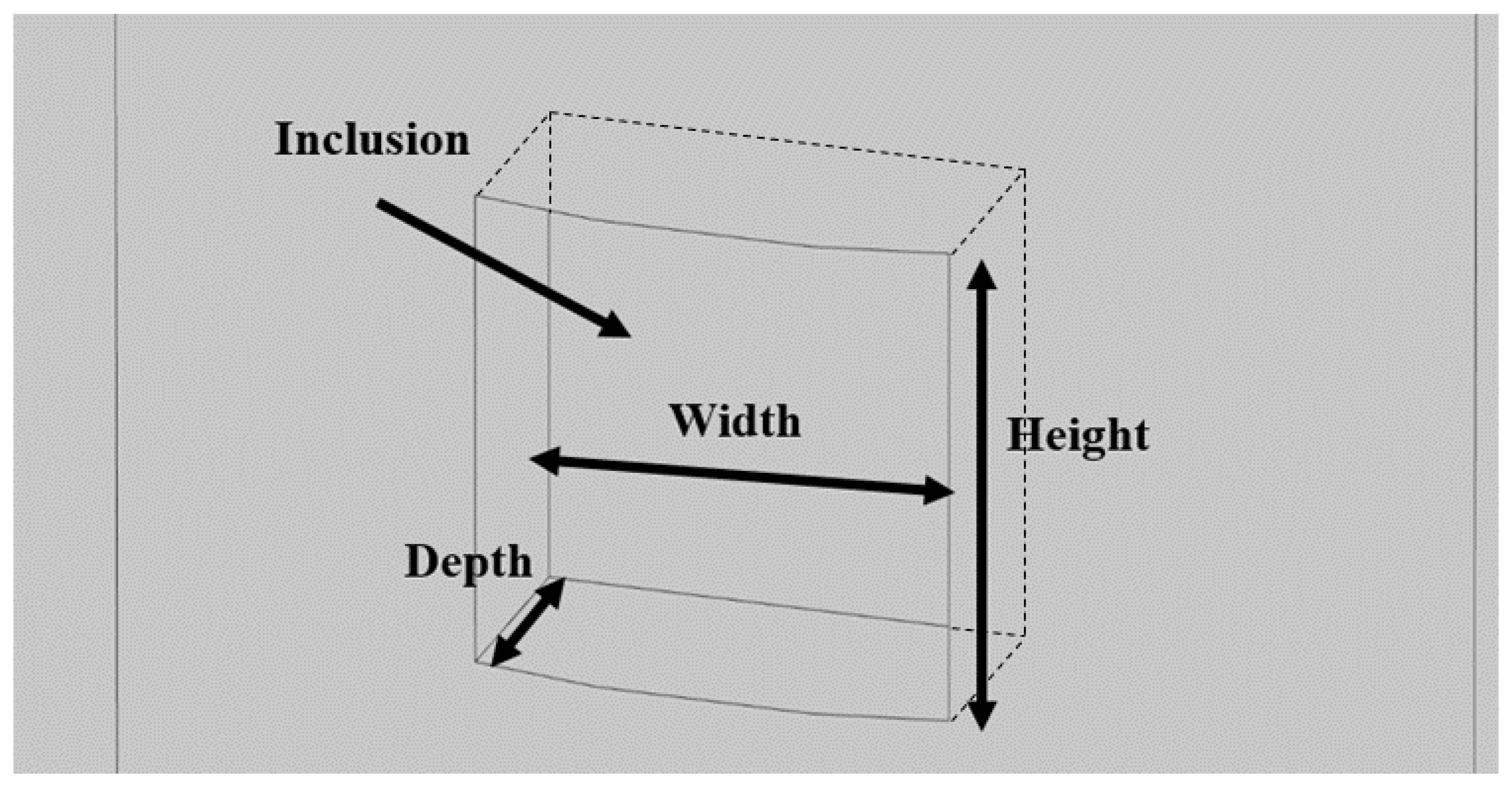
3.2. Void Defect
3.2.1. Forward Modeling
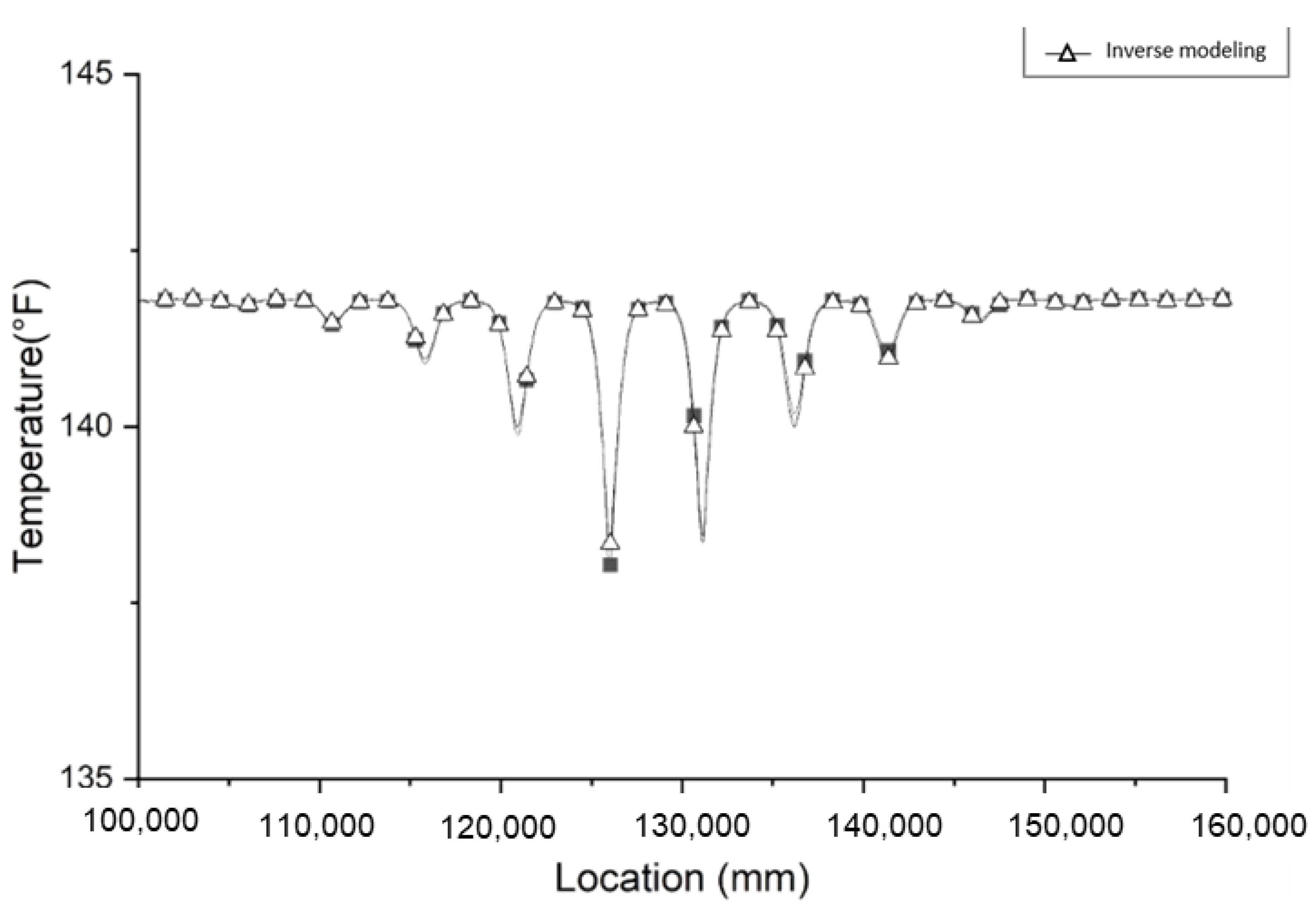
3.2.2. Inverse Modeling
4. Conclusions
Author Contributions
Funding
Institutional Review Board Statement
Informed Consent Statement
Data Availability Statement
Conflicts of Interest
References
- Mullins, G. Thermal integrity profiling of drilled shafts. DFI J. J. Deep Found. Inst. 2010, 4, 54–64. [Google Scholar] [CrossRef]
- Johnson, K.R. Analyzing thermal integrity profiling data for drilled shaft evaluation. DFI J. J. Deep Found. Inst. 2016, 10, 25–33. [Google Scholar] [CrossRef]
- Mullins, G.; Winters, D. Infrared Thermal Integrity Testing Quality Assurance Test Method to Detect Drilled Shaft Defects; Office of Research and Library Services: Washington, DC, USA, 2011. [Google Scholar]
- Mullins, G. Advancements in drilled shaft construction, design, and quality assurance: The value of research. Int. J. Pavement Res. Technol. 2013, 6, 93–99. [Google Scholar]
- Boeckmann, A.Z.; Loehr, J.E. Evaluation of thermal integrity profiling and crosshole sonic logging for drilled shafts with concrete defects. Transp. Res. Rec. 2019, 2673, 86–98. [Google Scholar] [CrossRef]
- Winters, D. In Comparative Study of Thermal Integrity Profiling with Other Nondestructive Integrity Test Methods for Drilled Shafts. In Proceedings of the Geo-Congress 2014: Geo-Characterization and Modeling for Sustainability, Atlanta, GA, USA, 23–26 February 2014; pp. 1731–1742. [Google Scholar]
- Schoen, D.L.; Canivan, G.J.; Camp, W.M., III. Evaluation of Thermal Integrity Profiling (TIP) Methods–Probe, Embedded Wire and Wire Suspended in CSL Tubes. In Proceedings of the IFCEE 2018, Orlando, FL, USA, 5–10 March 2018; pp. 550–560. [Google Scholar]
- Rui, Y.; Kechavarzi, C.; O’Leary, F.; Barker, C.; Nicholson, D.; Soga, K. Integrity testing of pile cover using distributed fibre optic sensing. Sensors 2017, 17, 2949. [Google Scholar] [CrossRef] [PubMed] [Green Version]
- Soga, K.; Luo, L. Distributed fiber optic sensors for civil engineering infrastructure sensing. J. Struct. Integr. Maint. 2018, 3, 1–21. [Google Scholar] [CrossRef]
- Minardo, A.; Bernini, R.; Amato, L.; Zeni, L. Bridge monitoring using Brillouin fiber-optic sensors. IEEE Sens. J. 2011, 12, 145–150. [Google Scholar] [CrossRef]
- Regier, R.; Hoult, N.A. Distributed strain behavior of a reinforced concrete bridge: Case study. J. Bridge Eng. 2014, 19, 05014007. [Google Scholar] [CrossRef]
- Webb, G.; Vardanega, P.; Hoult, N.; Fidler, P.; Bennett, P.; Middleton, C. Analysis of fiber-optic strain-monitoring data from a prestressed concrete bridge. J. Bridge Eng. 2017, 22, 05017002. [Google Scholar] [CrossRef] [Green Version]
- Xu, J.; Dong, Y.; Zhang, Z.; Li, S.; He, S.; Li, H. Full scale strain monitoring of a suspension bridge using high performance distributed fiber optic sensors. Meas. Sci. Technol. 2016, 27, 124017. [Google Scholar] [CrossRef]
- Damiano, E.; Avolio, B.; Minardo, A.; Olivares, L.; Picarelli, L.; Zeni, L. A laboratory study on the use of optical fibers for early detection of pre-failure slope movements in shallow granular soil deposits. Geotech. Test. J. 2017, 40, 529–541. [Google Scholar] [CrossRef]
- Hong, C.-Y.; Yin, J.-H.; Zhang, Y.-F. Deformation monitoring of long GFRP bar soil nails using distributed optical fiber sensing technology. Smart Mater. Struct. 2016, 25, 085044. [Google Scholar] [CrossRef]
- Sun, Y.; Shi, B.; Zhang, D.; Tong, H.; Wei, G.; Xu, H. Internal deformation monitoring of slope based on BOTDR. J. Sens. 2016, 2016, 8. [Google Scholar] [CrossRef]
- Xu, D.-S.; Yin, J.-H. Analysis of excavation induced stress distributions of GFRP anchors in a soil slope using distributed fiber optic sensors. Eng. Geol. 2016, 213, 55–63. [Google Scholar] [CrossRef]
- Schwamb, T.; Elshafie, M.Z.; Soga, K.; Mair, R.J. Considerations for monitoring of deep circular excavations. Proc. Inst. Civ. Eng. Geotech. Eng. 2016, 169, 477–493. [Google Scholar] [CrossRef] [Green Version]
- Schwamb, T.; Soga, K. Numerical modelling of a deep circular excavation at Abbey Mills in London. Géotechnique 2015, 65, 604–619. [Google Scholar] [CrossRef]
- Cheung, L.; Soga, K.; Bennett, P.J.; Kobayashi, Y.; Amatya, B.; Wright, P. Optical fibre strain measurement for tunnel lining monitoring. Proc. Inst. Civ. Eng. Geotech. Eng. 2010, 163, 119–130. [Google Scholar] [CrossRef]
- Alhaddad, M.; Wilcock, M.; Gue, C.; Bevan, H.; Stent, S.; Elshafie, M.Z.; Soga, K.; Devriendt, M.; Wright, P.; Waterfall, P. Multi-suite monitoring of an existing cast iron tunnel subjected to tunnelling-induced ground movements. In Proceedings of the Tunneling and Underground Construction, Shanghai, China, 26–28 May 2014; pp. 293–307. [Google Scholar]
- Luo, M.; Liu, J.; Tang, C.; Wang, X.; Lan, T.; Kan, B. 0.5 mm spatial resolution distributed fiber temperature and strain sensor with position-deviation compensation based on OFDR. Opt. Express 2019, 27, 35823–35829. [Google Scholar] [CrossRef] [PubMed]
- Zhong, R.; Guo, R.; Deng, W. Optical-fiber-based smart concrete thermal integrity profiling: An example of concrete shaft. Adv. Mater. Sci. Eng. 2018, 2018, 8. [Google Scholar] [CrossRef] [Green Version]
- Schindler, A.K.; Folliard, K.J. Heat of hydration models for cementitious materials. ACI Mater. J. 2005, 102, 24. [Google Scholar]
- Liu, W.; He, P.; Zhang, Z. A calculation method of thermal conductivity of soils. J. Glaciol. Geocryol. 2002, 24, 770–773. [Google Scholar]
- Sáez Blázquez, C.; Farfán Martín, A.; Martín Nieto, I.; Gonzalez-Aguilera, D. Measuring of thermal conductivities of soils and rocks to be used in the calculation of a geothermal installation. Energies 2017, 10, 795. [Google Scholar] [CrossRef]
- Abu-Hamdeh, N.H. Thermal properties of soils as affected by density and water content. Biosyst. Eng. 2003, 86, 97–102. [Google Scholar] [CrossRef]
- Winters, D.; Mullins, G. In Thermal Integrity Profiling of Concrete Deep Foundations. In Proceedings of the Geo-Construction Conference/ADSC Expo 2012, Oakland, CA, USA, 25–29 March 2012; pp. 155–165. [Google Scholar]
- Young, R.; Warkentin, B. Soil Properties and Behaviour; Elsevier: Amsterdam, The Netherlands, 1975. [Google Scholar]
- Neville, A.M. Properties of Concrete, 5th ed.; Pearson: New York, NY, USA, 2011. [Google Scholar]
- Iskander, M.; Roy, D.; Kelley, S.; Ealy, C. Drilled shaft defects: Detection, and effects on capacity in varved clay. J. Geotech. Geoenviron. Eng. 2003, 129, 1128–1137. [Google Scholar] [CrossRef]


| Soil Properties | Unit | Value |
| Density | kg/m3 | 1800 |
| Soil solid thermal conductivity | 5 | |
| Water thermal conductivity | 0.5 | |
| Air thermal conductivity | 0.05 | |
| Soil solid heat capacity | 850 | |
| Water heat capacity | 4190 | |
| Porosity | % | 51.1 |
| Water Content | % | 39.8 |
| Saturation | % | 97 |
| Concrete Properties | Unit | Value |
| Density | kg/m3 | 2300 |
| Thermal conductivity | 1.8 | |
| Heat capacity | 880 | |
| Heat generation rate | 2137.2e−0.9t (t is in days) |
Publisher’s Note: MDPI stays neutral with regard to jurisdictional claims in published maps and institutional affiliations. |
© 2021 by the authors. Licensee MDPI, Basel, Switzerland. This article is an open access article distributed under the terms and conditions of the Creative Commons Attribution (CC BY) license (https://creativecommons.org/licenses/by/4.0/).
Share and Cite
Deng, W.; Zhong, R.; Ma, H. Fiber Optic-Based Thermal Integrity Profiling of Drilled Shaft: Inverse Modeling for Spiral Fiber Deployment Strategy. Materials 2021, 14, 5377. https://doi.org/10.3390/ma14185377
Deng W, Zhong R, Ma H. Fiber Optic-Based Thermal Integrity Profiling of Drilled Shaft: Inverse Modeling for Spiral Fiber Deployment Strategy. Materials. 2021; 14(18):5377. https://doi.org/10.3390/ma14185377
Chicago/Turabian StyleDeng, Wen, Ruoyu Zhong, and Haiying Ma. 2021. "Fiber Optic-Based Thermal Integrity Profiling of Drilled Shaft: Inverse Modeling for Spiral Fiber Deployment Strategy" Materials 14, no. 18: 5377. https://doi.org/10.3390/ma14185377
APA StyleDeng, W., Zhong, R., & Ma, H. (2021). Fiber Optic-Based Thermal Integrity Profiling of Drilled Shaft: Inverse Modeling for Spiral Fiber Deployment Strategy. Materials, 14(18), 5377. https://doi.org/10.3390/ma14185377