
A Comparative Study for the Prediction of the Compressive Strength of Self-Compacting Concrete Modified with Fly Ash

 ,
,  ,
,  ,
,  ,
,  , , and
Abstract
:1. Introduction
2. Research Significance
3. Prediction Methods
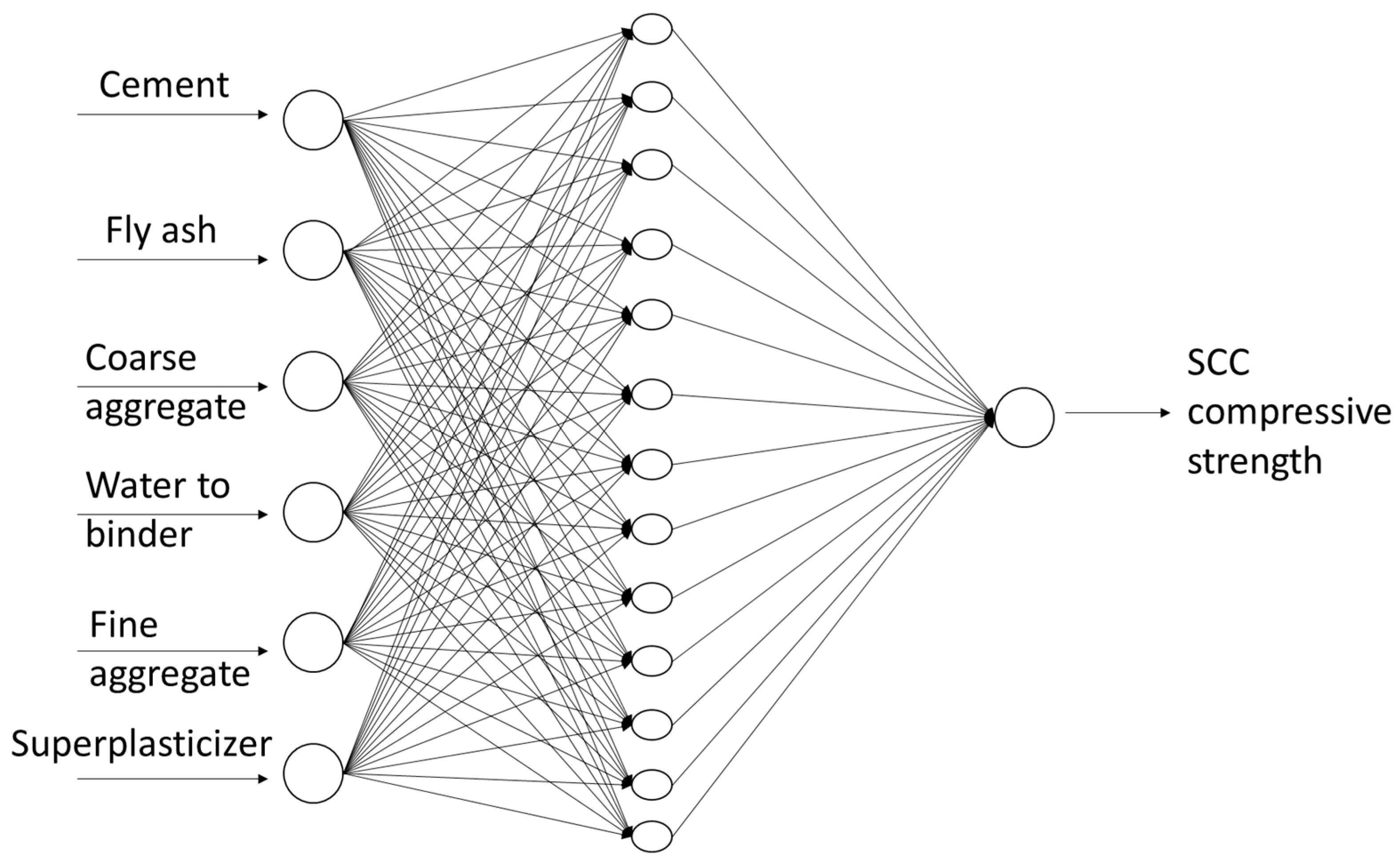
3.1. Artificial Neural Network (ANNs)
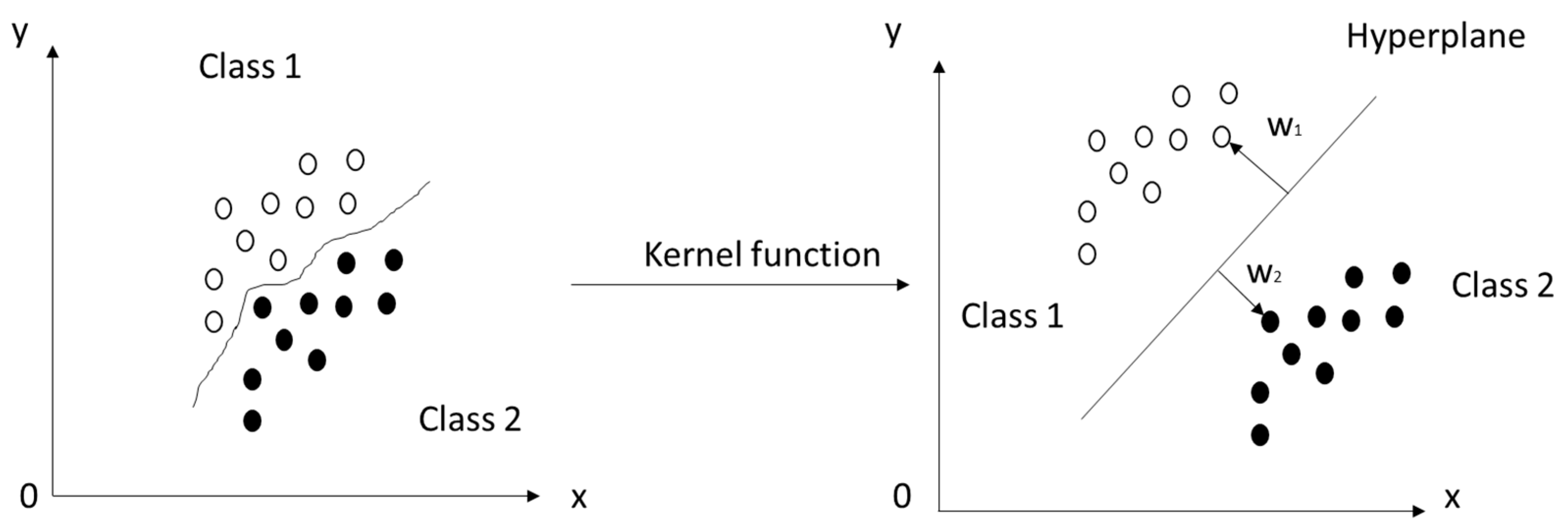
3.2. Support Vector Machine (SVM)
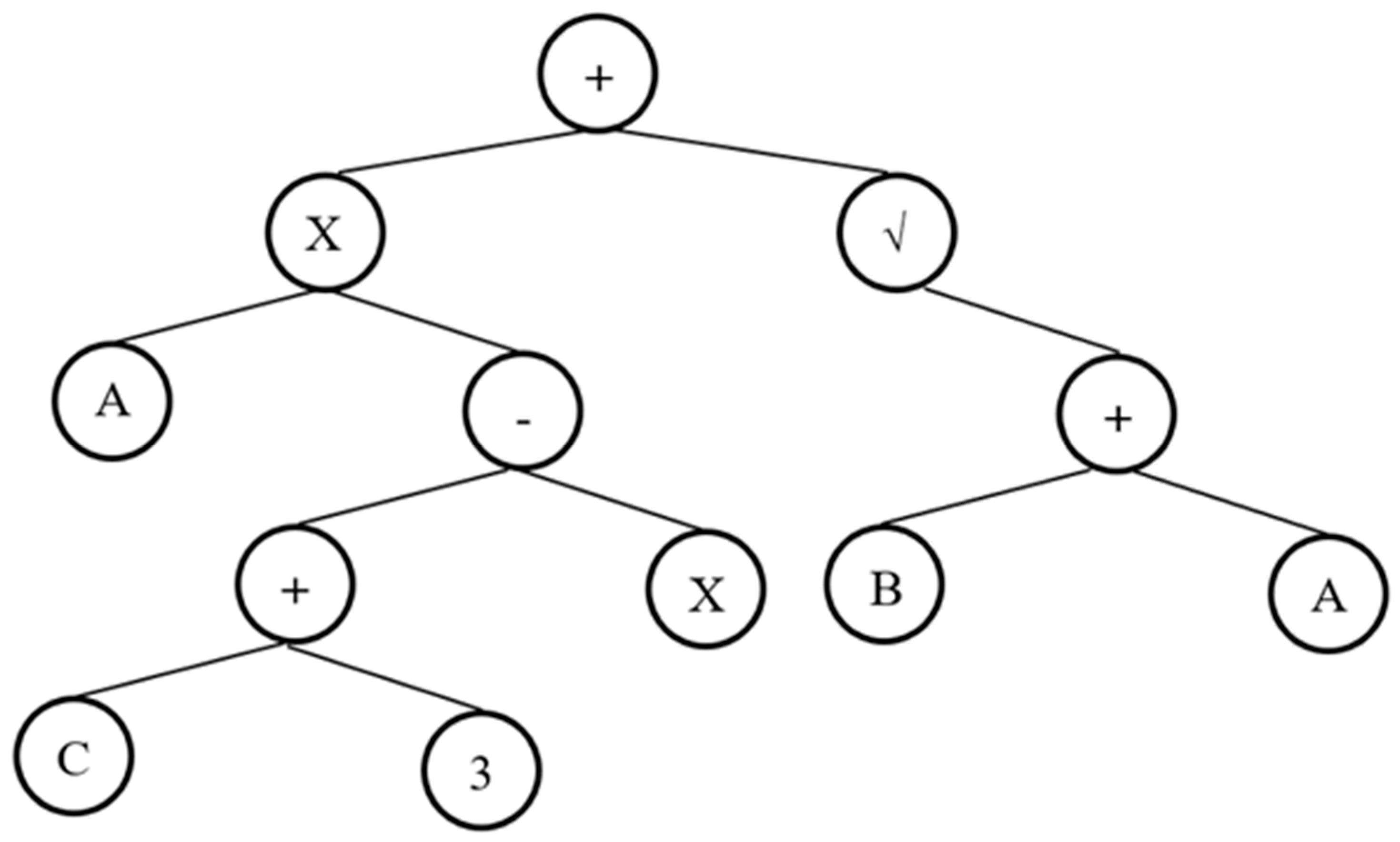
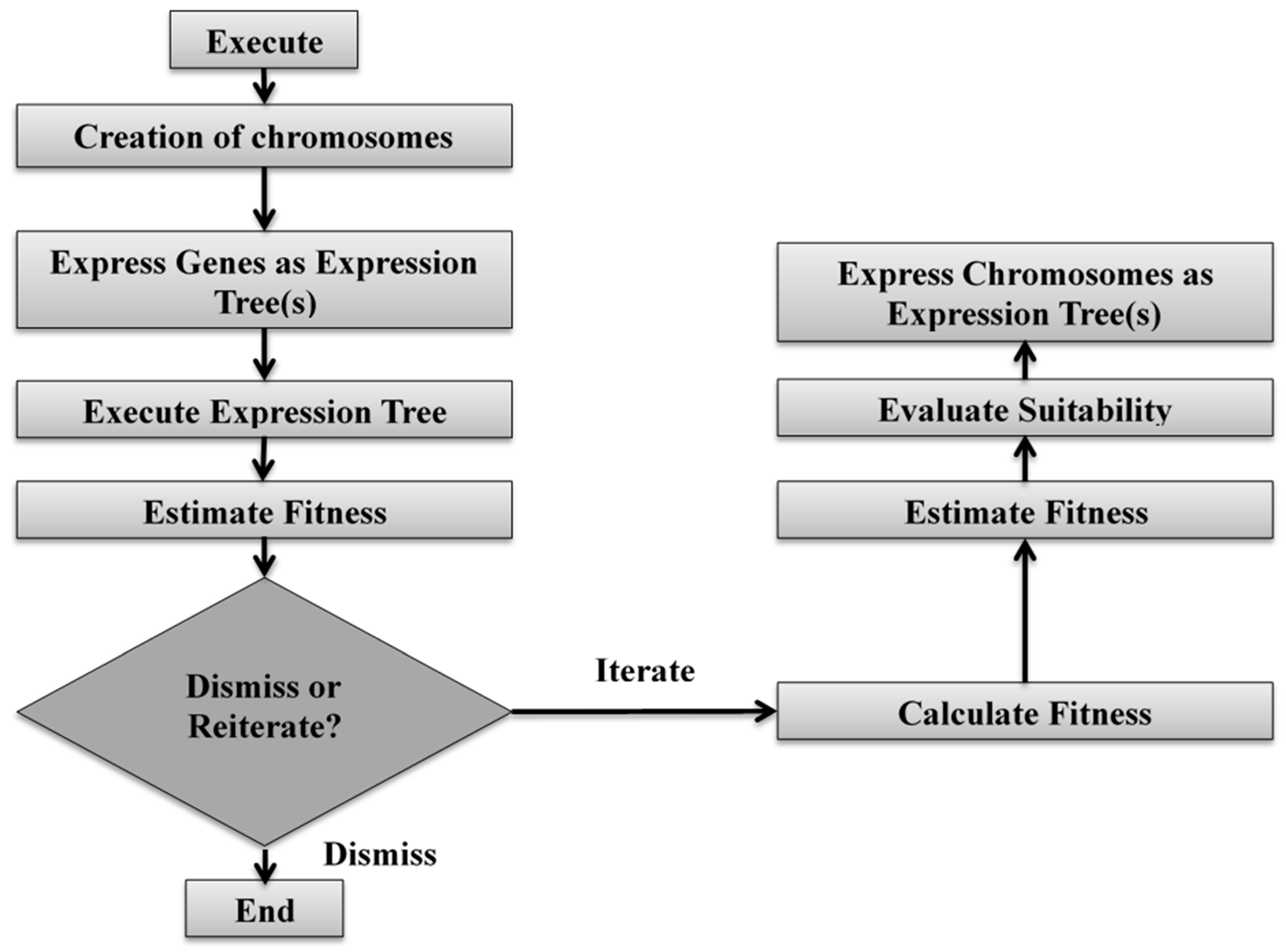
3.3. Genetic Engineering Programming (GEP)
4. Data Presentation
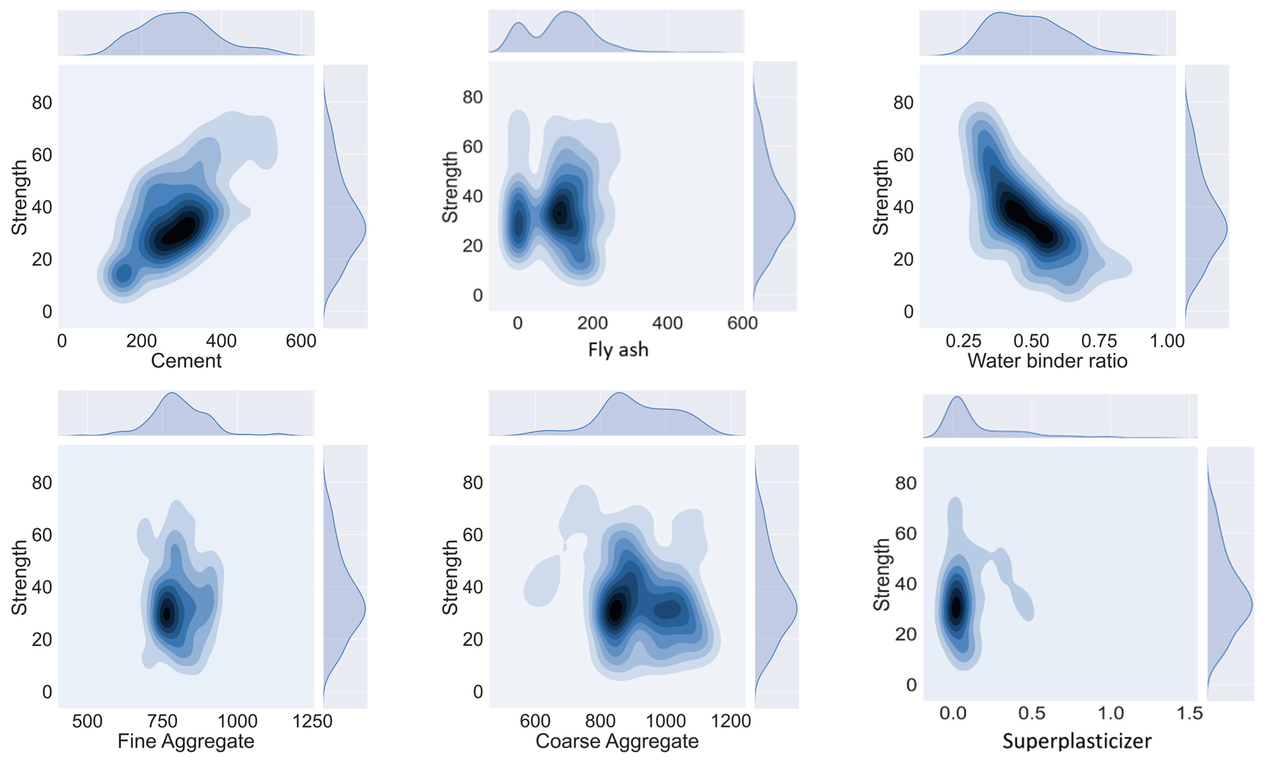
4.1. Correlation Graph Python Programming Based
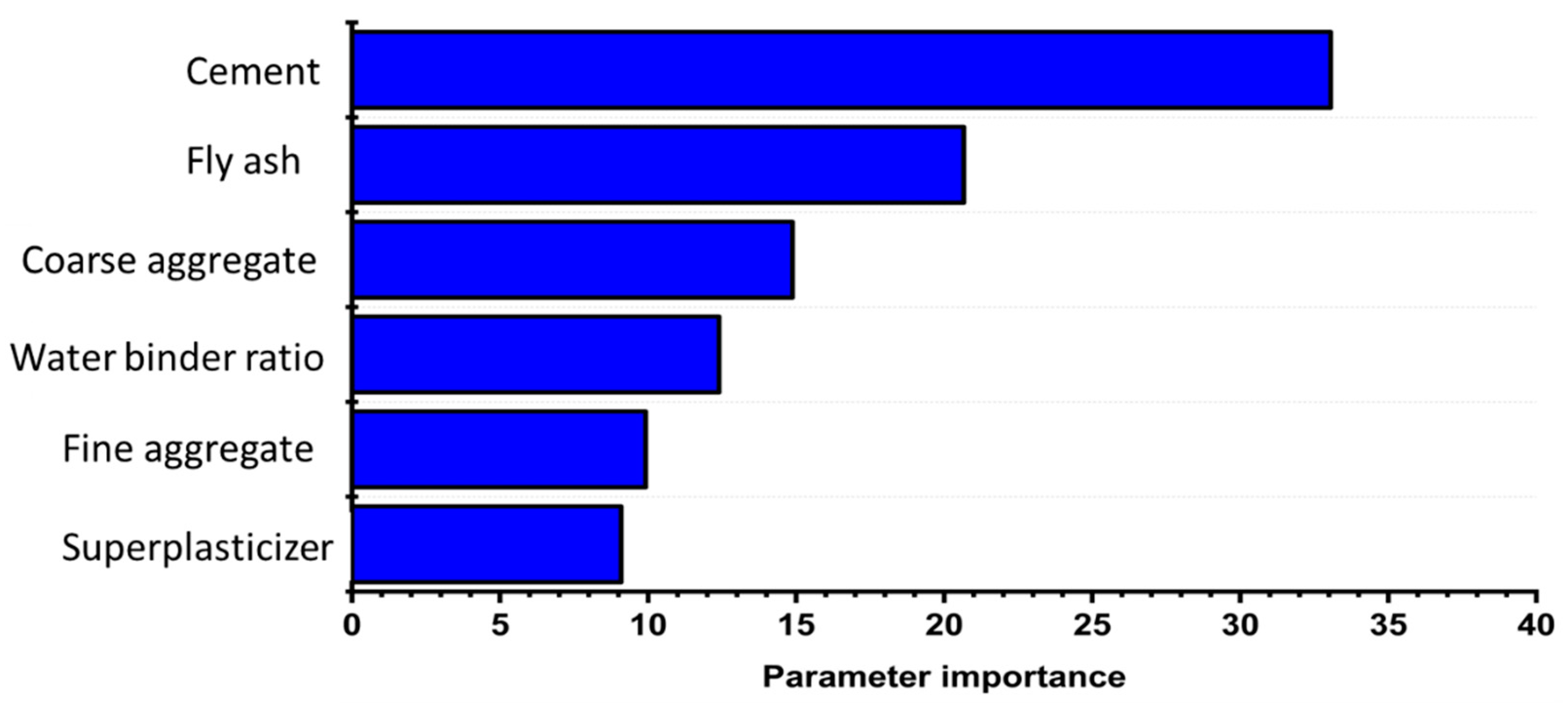
4.2. Sensitivity Analysis or Permutation Feature Importance
5. Results and Discussion
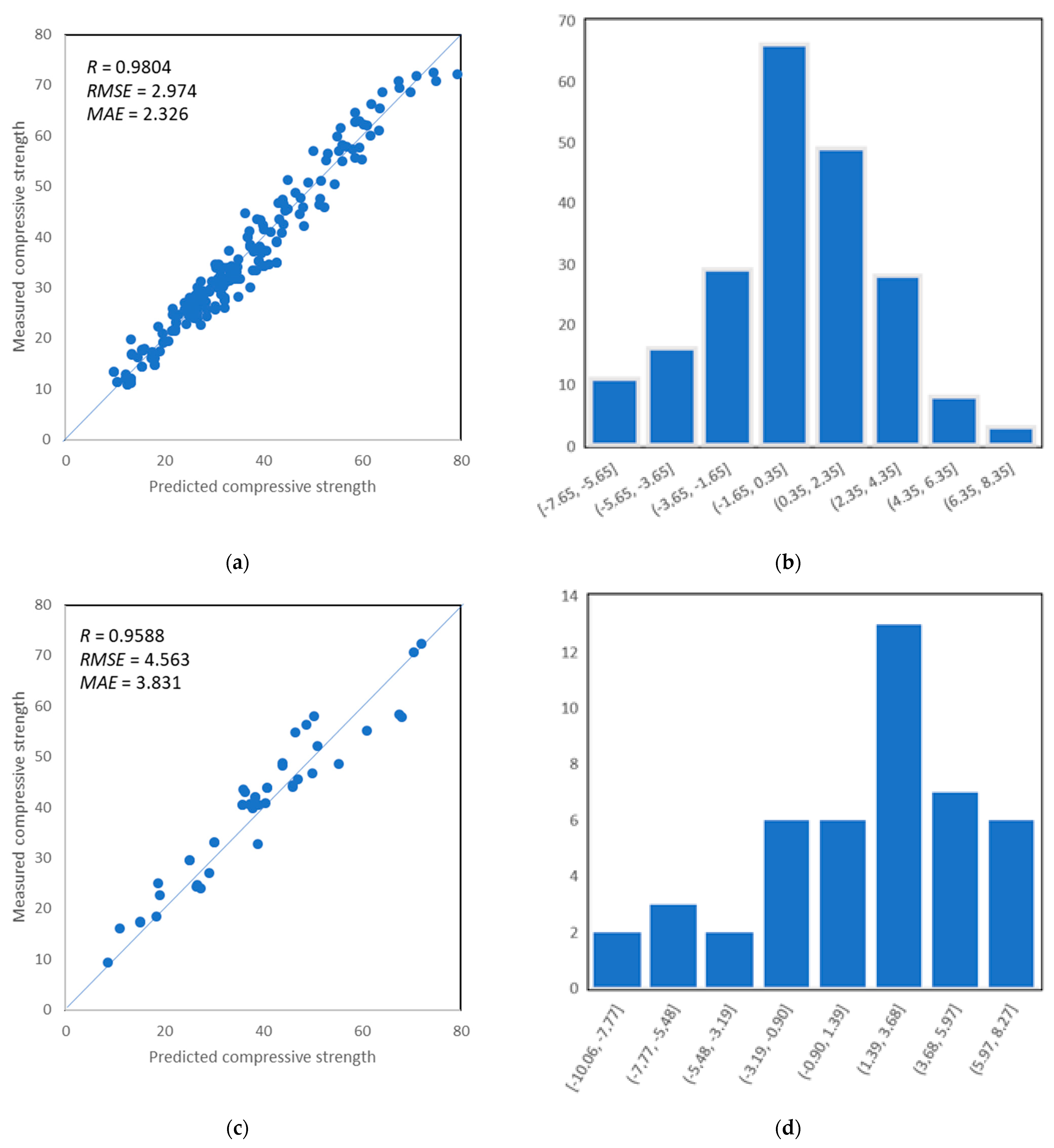
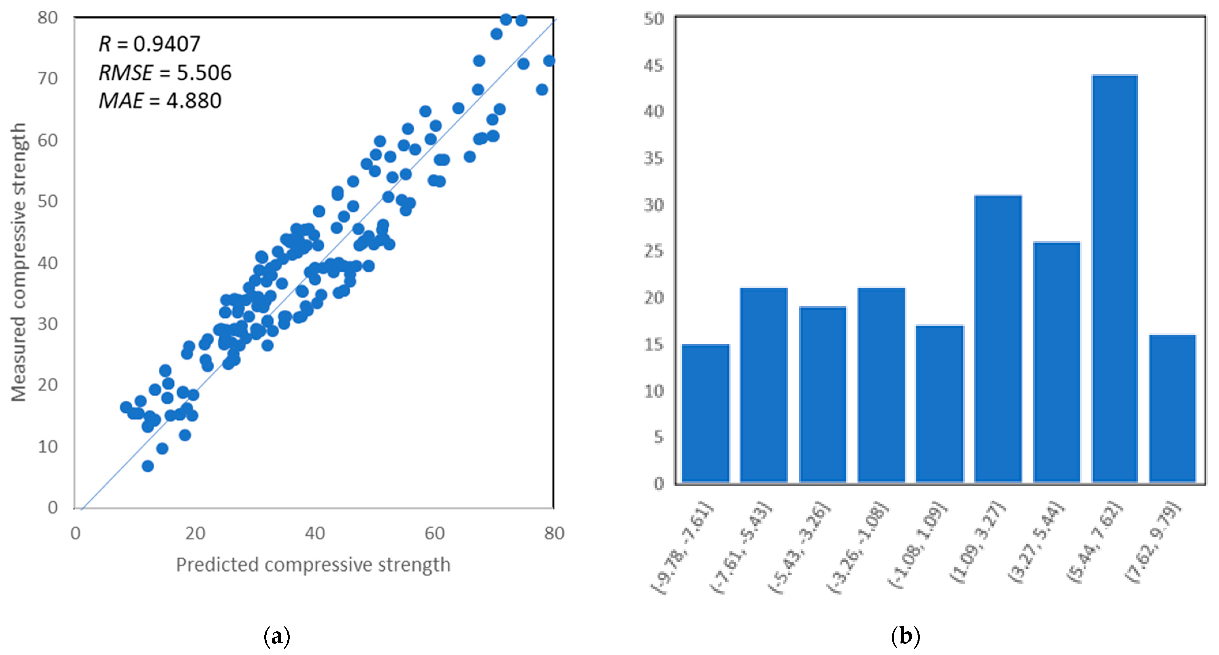
5.1. Artificial Neural Network
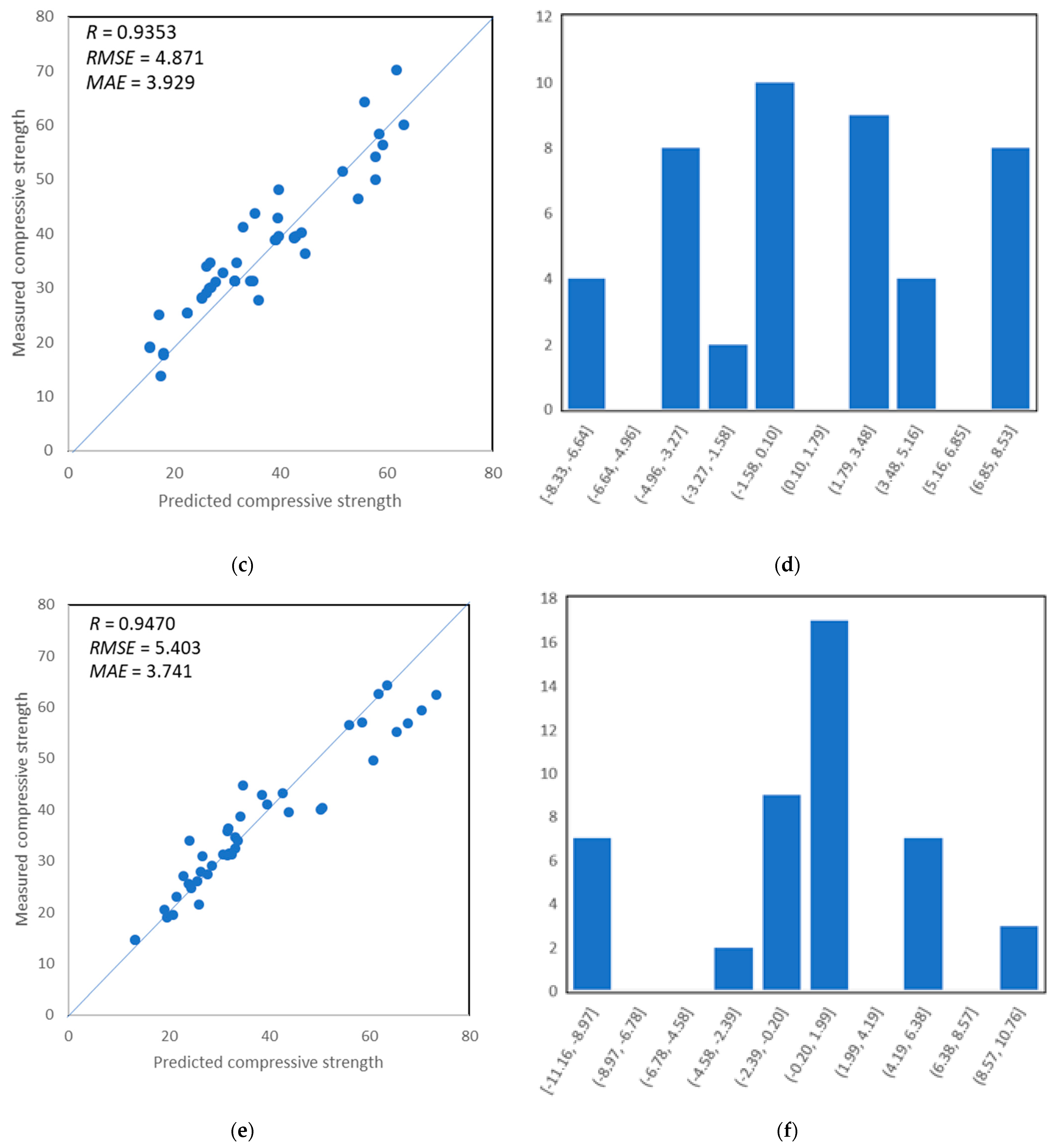
5.2. Support Vector Machine
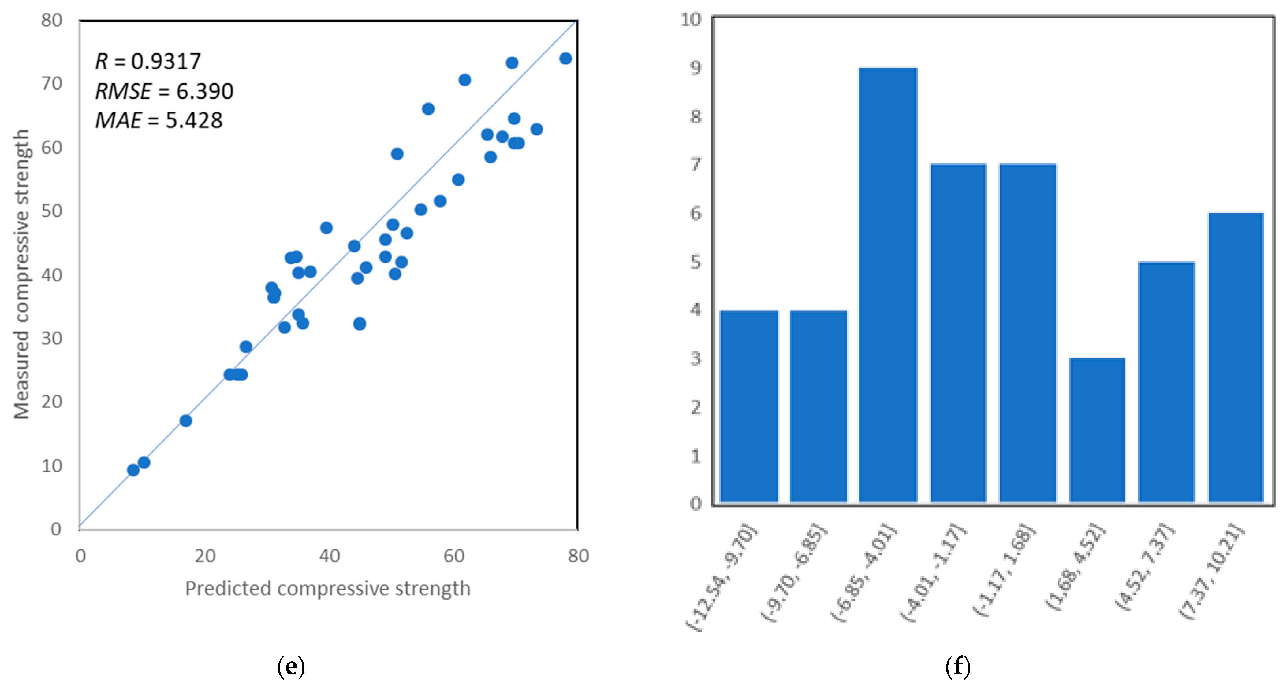
5.3. Gene Expression Programming
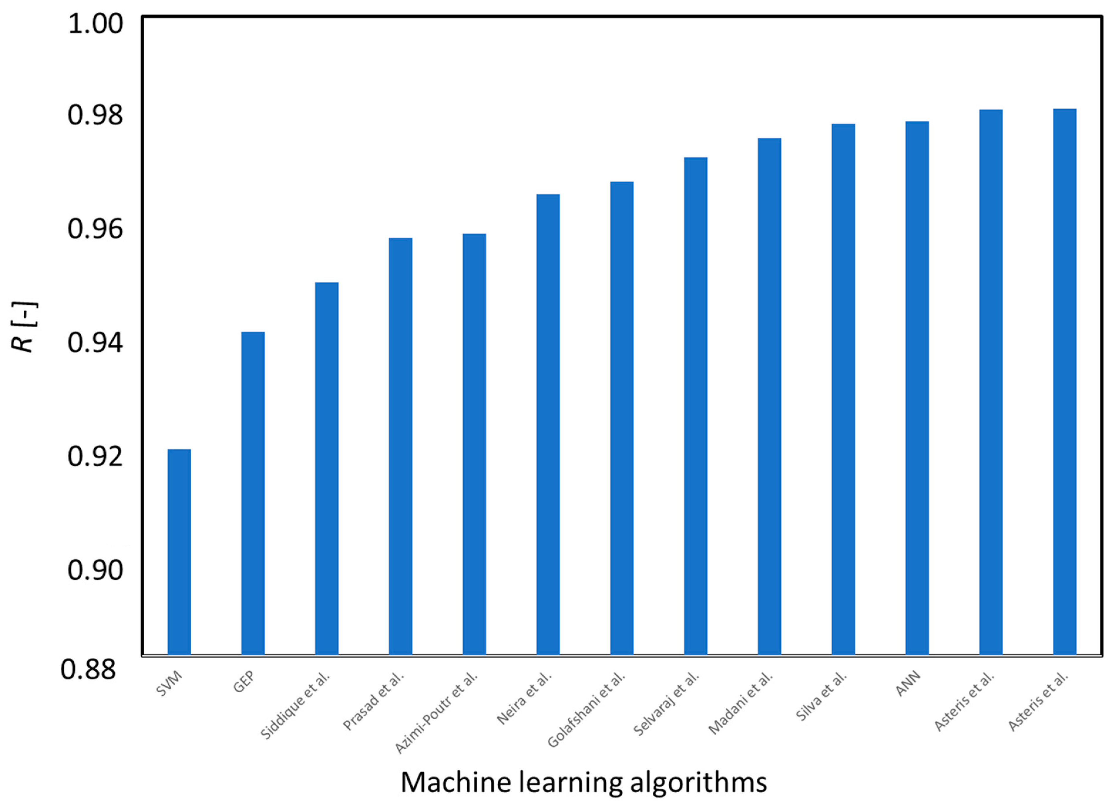
5.4. Comparison between the Proposed Models
6. Conclusions
- ANN-, SVM-, and GEP-based models predict the properties of SCC strength; however, ANN and GEP are the most accurate for this purpose;
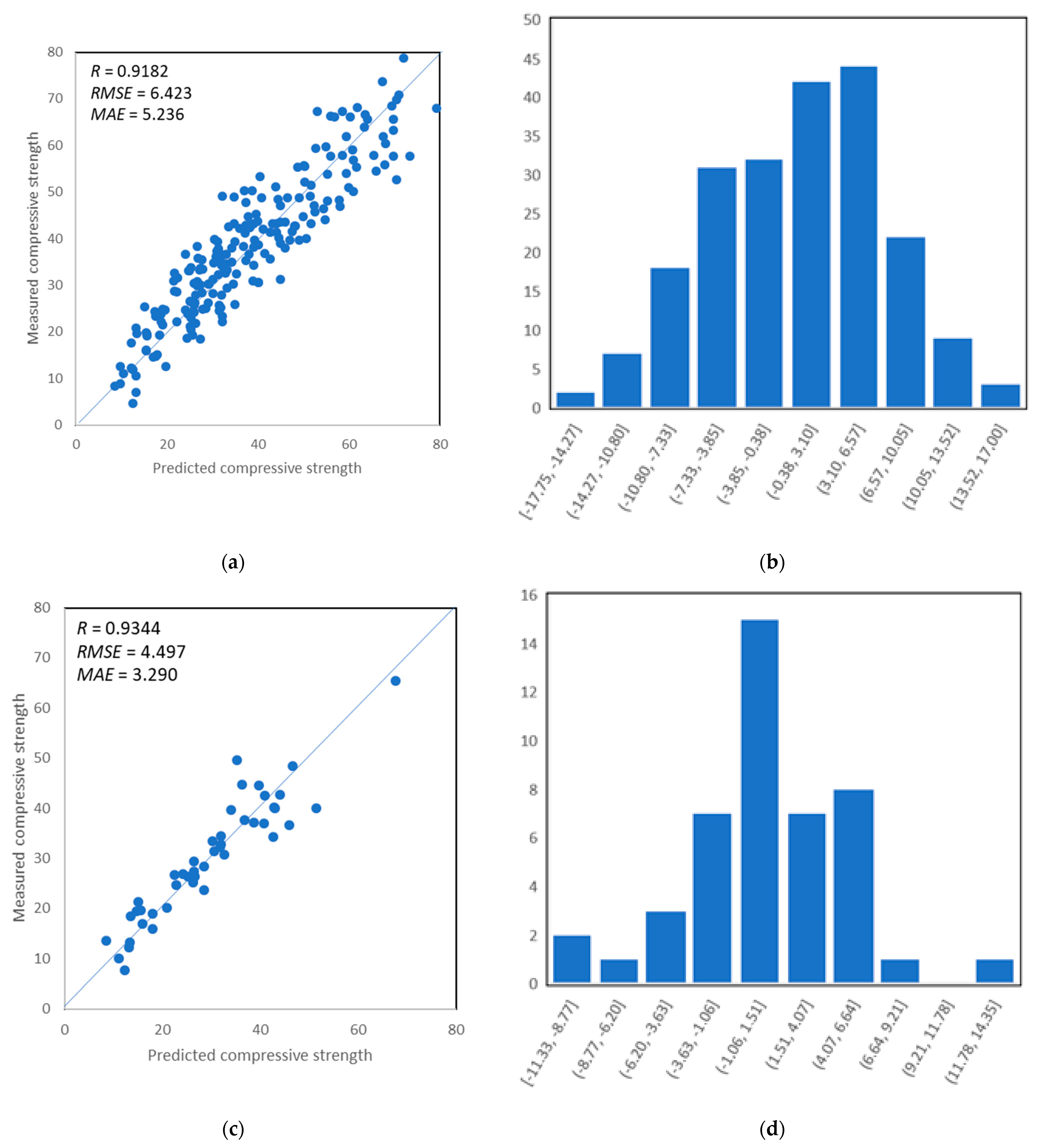
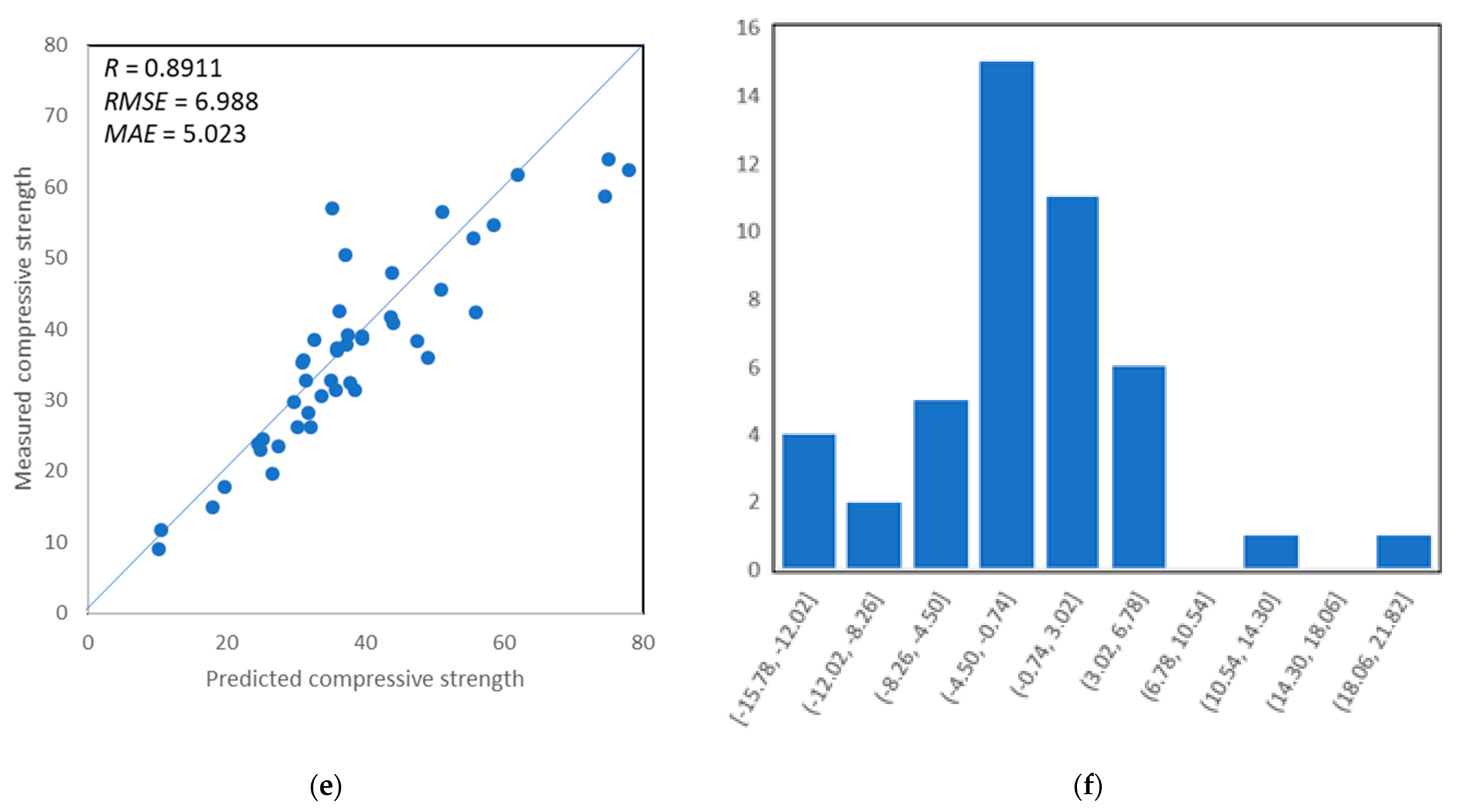
- ANN, SVM, and GEP models were characterized by the very high values of linear correlation coefficient equal to R = 0.9588, R = 0.9344 and R = 0.9353 for the testing set, respectively. The test set of the ANN, SVM, and GEP models show average error values of 5.428 MPa, 5.023 MPa, and 3.741 MPa, respectively. This indicates that the GEP model was able to be performed better in terms of accuracy during this process in comparison to the ANN and SVM models;
- Permutation features show clear influential parameters for strength prediction. Variable such as the ratio of cement and fly ash added to the mixture have a major effect on strength with 53% out of total parameters. Thus, it is important to know their ratio in the mixture in order to evaluate the SCC compressive strength; without this variable, the modelling might be less accurate;
- Statistical analysis and external checks give obstinate responses for all models.
- Hybrid models or advanced evolutionary algorithms can be developed, and the results can be compared to the present study.
- The techniques used in this study can be used to model other engineering properties of concrete and structures.
- Sometimes, the GEP is trapped in a local region that does not contain the global optimum. This phenomenon is called premature convergence and is one of the serious problems in genetic algorithms.
- The “best” fitness is in comparison to other fitness; i.e., the stop criterion is not clear in every problem.
- For specific optimization problems and problem instances, other optimization algorithms may be more efficient than genetic algorithms in terms of speed of convergence.
Author Contributions
Funding
Institutional Review Board Statement
Informed Consent Statement
Data Availability Statement
Conflicts of Interest
Appendix A

| No. | Cement | Fly Ash | Water–Powder Ratio | Sand | Coarse Aggregate | Superplasticizer | Strength |
|---|---|---|---|---|---|---|---|
| - | kg/m3 | kg/m3 | - | kg/m3 | kg/m3 | kg/m3 | MPa |
| 1 | 148 | 137 | 0.55 | 830 | 1002 | 0.11 | 17.95 |
| 2 | 393 | 0 | 0.49 | 758 | 940 | 0 | 39.58 |
| 3 | 325 | 60 | 0.65 | 900 | 850 | 0.12 | 31.4 |
| 4 | 374.3 | 0 | 0.51 | 730.4 | 1013.2 | 0.02 | 39.06 |
| 5 | 348 | 224 | 0.5 | 783 | 848 | 0.43 | 58.6 |
| 6 | 296 | 107 | 0.55 | 778 | 819 | 0.04 | 31.42 |
| 7 | 350 | 162 | 0.41 | 768 | 840 | 0.18 | 51.7 |
| 8 | 296 | 106.7 | 0.55 | 778.4 | 819.2 | 0.04 | 31.42 |
| 9 | 374 | 0 | 0.51 | 730 | 1013 | 0.02 | 39.05 |
| 10 | 148.1 | 136.6 | 0.56 | 830.1 | 1001.8 | 0.11 | 17.96 |
| 11 | 275 | 0 | 0.67 | 808 | 1088 | 0 | 24.5 |
| 12 | 231.75 | 121.62 | 0.49 | 778.45 | 1056.4 | 0.03 | 33.73 |
| 13 | 181.38 | 167.01 | 0.49 | 777.8 | 1055.6 | 0.04 | 27.77 |
| 14 | 194.68 | 100.52 | 0.56 | 905.9 | 1006.4 | 0.04 | 25.72 |
| 15 | 325 | 60 | 0.65 | 899 | 850 | 0.43 | 30.8 |
| 16 | 420 | 80 | 0.33 | 785 | 860 | 0.3 | 56 |
| 17 | 212.52 | 100.37 | 0.51 | 903.59 | 1007.8 | 0.04 | 31.64 |
| 18 | 290 | 100 | 0.33 | 913 | 837 | 0.01 | 42.7 |
| 19 | 333 | 0 | 0.58 | 842.6 | 931.2 | 0 | 31.97 |
| 20 | 250 | 160 | 0.55 | 742 | 837 | 0.5 | 28.5 |
| 21 | 339 | 0 | 0.58 | 781 | 968 | 0 | 32.04 |
| 22 | 207 | 207 | 0.45 | 845 | 843 | 0.4 | 33.2 |
| 23 | 252 | 0 | 0.73 | 784 | 1111 | 0 | 19.69 |
| 24 | 360 | 240 | 0.28 | 853 | 698 | 0.3 | 63.5 |
| 25 | 417 | 153 | 0.32 | 828 | 759 | 0.31 | 61.82 |
| 26 | 163 | 245 | 0.4 | 851 | 851 | 0.2 | 26.2 |
| 27 | 310 | 0 | 0.62 | 850 | 970 | 0 | 27.92 |
| 28 | 350 | 133 | 0.38 | 815 | 883 | 0.34 | 55.3 |
| 29 | 190.34 | 125.18 | 0.51 | 802.59 | 1088.1 | 0.05 | 28.47 |
| 30 | 427 | 115 | 0.36 | 779 | 844 | 0.26 | 59.4 |
| 31 | 475 | 0 | 0.48 | 594 | 932 | 0 | 39.29 |
| 32 | 164.6 | 150.4 | 0.58 | 728.9 | 1023.3 | 0.07 | 18.03 |
| 33 | 165 | 150 | 0.58 | 729 | 1023 | 0.07 | 18.03 |
| 34 | 318 | 126 | 0.47 | 737 | 861 | 0.02 | 40.06 |
| 35 | 317.9 | 126.5 | 0.47 | 736.6 | 860.5 | 0.02 | 40.06 |
| 36 | 280 | 96 | 0.87 | 817 | 850 | 0.62 | 15.9 |
| 37 | 540 | 0 | 0.32 | 613 | 1125 | 0 | 67.31 |
| 38 | 183 | 160 | 0.55 | 891 | 837 | 0.5 | 22.1 |
| 39 | 238.05 | 94.11 | 0.56 | 847.01 | 949.91 | 0.03 | 30.23 |
| 40 | 307 | 0 | 0.63 | 812 | 968 | 0 | 27.53 |
| 41 | 480 | 96 | 0.38 | 819 | 699 | 0.94 | 53 |
| 42 | 144.8 | 133.6 | 0.65 | 811.5 | 979.5 | 0.08 | 13.2 |
| 43 | 145 | 134 | 0.65 | 812 | 979 | 0.08 | 13.2 |
| 44 | 151.6 | 111.9 | 0.7 | 815.9 | 992 | 0.05 | 12.18 |
| 45 | 325 | 60 | 0.85 | 722 | 850 | 0.43 | 13.3 |
| 46 | 370 | 24 | 0.69 | 772 | 850 | 0.25 | 26.4 |
| 47 | 152 | 112 | 0.7 | 816 | 992 | 0.05 | 12.18 |
| 48 | 331 | 0 | 0.58 | 825 | 978 | 0 | 31.45 |
| 49 | 252.5 | 0 | 0.74 | 784.3 | 1111.6 | 0 | 19.77 |
| 50 | 505 | 60 | 0.35 | 630 | 1030 | 0 | 64.02 |
| 51 | 134.7 | 165.7 | 0.6 | 804.9 | 961 | 0.07 | 13.29 |
| 52 | 325 | 60 | 0.65 | 899 | 850 | 0.43 | 32.6 |
| 53 | 135 | 166 | 0.6 | 805 | 961 | 0.07 | 13.29 |
| 54 | 475 | 0 | 0.34 | 662 | 1044 | 0.02 | 58.52 |
| 55 | 251.37 | 118.27 | 0.52 | 754.3 | 1043.6 | 0.02 | 33.27 |
| 56 | 166.09 | 163.27 | 0.54 | 780.09 | 1058.6 | 0.03 | 21.54 |
| 57 | 393 | 0 | 0.49 | 785.6 | 940.6 | 0 | 39.6 |
| 58 | 250 | 0 | 0.73 | 820 | 1100 | 0 | 20.87 |
| 59 | 210 | 100 | 0.65 | 910 | 837 | 0.8 | 19.1 |
| 60 | 190.68 | 125.4 | 0.51 | 804.01 | 1090 | 0.04 | 26.4 |
| 61 | 249 | 60 | 0.68 | 1079 | 850 | 0.43 | 24 |
| 62 | 405 | 0 | 0.43 | 695 | 1120 | 0 | 52.3 |
| 63 | 528 | 0 | 0.35 | 720 | 920 | 0.01 | 56.83 |
| 64 | 250 | 160 | 0.55 | 739 | 837 | 0 | 27.3 |
| 65 | 273 | 90 | 0.55 | 762 | 931 | 0.04 | 32.24 |
| 66 | 297.16 | 117.54 | 0.42 | 753.45 | 1022.8 | 0.03 | 47.4 |
| 67 | 169 | 254 | 0.45 | 853 | 853 | 0 | 30.2 |
| 68 | 272.6 | 89.6 | 0.55 | 762.2 | 931.3 | 0.04 | 32.25 |
| 69 | 190.34 | 125.18 | 0.53 | 798.9 | 1079 | 0.05 | 24.85 |
| 70 | 310 | 0 | 0.62 | 830 | 1012 | 0 | 27.83 |
| 71 | 298 | 107 | 0.52 | 744 | 880 | 0.04 | 31.87 |
| 72 | 298.2 | 107 | 0.52 | 744.2 | 879.6 | 0.04 | 31.88 |
| 73 | 251.37 | 118.27 | 0.51 | 757.73 | 1028.4 | 0.03 | 32.66 |
| 74 | 247 | 165 | 0.45 | 845 | 846 | 0.12 | 34.6 |
| 75 | 400 | 0 | 0.47 | 745 | 1025 | 0 | 43.7 |
| 76 | 170 | 200 | 0.43 | 930 | 900 | 0.2 | 31 |
| 77 | 289 | 0 | 0.66 | 895.3 | 913.2 | 0 | 25.57 |
| 78 | 317 | 160 | 0.55 | 594 | 837 | 0.5 | 29.1 |
| 79 | 326 | 138 | 0.43 | 792 | 801 | 0.03 | 40.68 |
| 80 | 295 | 0 | 0.63 | 769 | 1069 | 0 | 25.18 |
| 81 | 520 | 0 | 0.33 | 855 | 855 | 0.01 | 60.28 |
| 82 | 225 | 275 | 0.35 | 908 | 652 | 0.7 | 41.42 |
| 83 | 222.36 | 96.67 | 0.59 | 870.32 | 967.08 | 0.02 | 24.89 |
| 84 | 165 | 143.57 | 0.53 | 900.9 | 1005.6 | 0 | 26.2 |
| 85 | 238 | 0 | 0.78 | 789 | 1119 | 0 | 17.54 |
| 86 | 238 | 0 | 0.78 | 789 | 1118 | 0 | 17.54 |
| 87 | 238.1 | 0 | 0.78 | 789.3 | 1118.8 | 0 | 17.58 |
| 88 | 238 | 159 | 0.4 | 844 | 844 | 0.29 | 37.8 |
| 89 | 522 | 0 | 0.28 | 896 | 896 | 0 | 74.99 |
| 90 | 148 | 182 | 0.55 | 884 | 839 | 0.1 | 15.52 |
| 91 | 290 | 100 | 0.65 | 709 | 837 | 0.2 | 26.6 |
| 92 | 148.1 | 182.1 | 0.55 | 884.3 | 838.9 | 0.1 | 15.53 |
| 93 | 154.8 | 142.8 | 0.65 | 696.7 | 1047.4 | 0.06 | 12.46 |
| 94 | 302 | 0 | 0.67 | 817 | 974 | 0 | 21.75 |
| 95 | 155 | 143 | 0.65 | 697 | 1047 | 0.06 | 12.46 |
| 96 | 280 | 120 | 0.39 | 946 | 900 | 0.35 | 45 |
| 97 | 255 | 0 | 0.75 | 945 | 889.8 | 0 | 18.75 |
| 98 | 250 | 160 | 0.55 | 746 | 837 | 1 | 26.7 |
| 99 | 400 | 60 | 0.63 | 718 | 850 | 0.43 | 30.4 |
| 100 | 322 | 0 | 0.63 | 800 | 974 | 0 | 25.18 |
| 101 | 250 | 160 | 0.55 | 742 | 837 | 0.5 | 26.4 |
| 102 | 220 | 180 | 0.45 | 850 | 900 | 0.35 | 38 |
| 103 | 350 | 90 | 0.48 | 852 | 923 | 0.14 | 46.5 |
| 104 | 290 | 100 | 0.45 | 913 | 837 | 0.8 | 42.7 |
| 105 | 213.74 | 174.74 | 0.4 | 776.35 | 1053.5 | 0.05 | 40.15 |
| 106 | 331 | 0 | 0.58 | 821 | 1025 | 0 | 31.74 |
| 107 | 427 | 115 | 0.45 | 779 | 844 | 0.12 | 59.4 |
| 108 | 295.8 | 0 | 0.63 | 769.3 | 1091.4 | 0 | 25.22 |
| 109 | 281 | 0 | 0.66 | 774 | 1104 | 0 | 22.44 |
| 110 | 281 | 0 | 0.66 | 774 | 1104 | 0 | 22.44 |
| 111 | 296 | 0 | 0.63 | 769 | 1090 | 0 | 25.18 |
| 112 | 325 | 60 | 0.65 | 898 | 850 | 0.43 | 34.3 |
| 113 | 250 | 160 | 0.55 | 742 | 837 | 0.5 | 26 |
| 114 | 275 | 275 | 0.37 | 796 | 937 | 0.74 | 63.32 |
| 115 | 300 | 0 | 0.61 | 795 | 1075 | 0 | 26.85 |
| 116 | 298.1 | 107 | 0.46 | 815.2 | 879 | 0.02 | 42.64 |
| 117 | 298 | 107 | 0.46 | 815 | 879 | 0.02 | 42.64 |
| 118 | 290 | 100 | 0.48 | 709 | 837 | 0 | 26.6 |
| 119 | 325 | 60 | 0.65 | 896 | 850 | 0.75 | 27.7 |
| 120 | 220 | 180 | 0.39 | 916 | 900 | 0.6 | 43 |
| 121 | 370 | 96 | 0.57 | 833 | 850 | 0.25 | 39.5 |
| 122 | 225 | 0 | 0.8 | 833 | 1113 | 0 | 17.34 |
| 123 | 200 | 200 | 0.4 | 842 | 843 | 0.17 | 34.9 |
| 124 | 143.6 | 174.9 | 0.5 | 844.5 | 942.7 | 0.12 | 15.42 |
| 125 | 250 | 95.69 | 0.54 | 861.17 | 956.86 | 0.02 | 29.22 |
| 126 | 144 | 175 | 0.5 | 844 | 943 | 0.13 | 15.42 |
| 127 | 322 | 138 | 0.35 | 693.81 | 1085.2 | 0 | 58 |
| 128 | 322.5 | 107.5 | 0.47 | 1135 | 630 | 0.01 | 43.98 |
| 129 | 325 | 60 | 0.65 | 898 | 850 | 0.43 | 35 |
| 130 | 250 | 160 | 0.55 | 742 | 837 | 0.5 | 25.3 |
| 131 | 212.07 | 121.62 | 0.54 | 779.32 | 1057.6 | 0.03 | 24.9 |
| 132 | 301 | 129 | 0.47 | 1135 | 630 | 0.01 | 44 |
| 133 | 325 | 0 | 0.57 | 783 | 1063 | 0 | 30.57 |
| 134 | 218.85 | 124.13 | 0.46 | 794.91 | 1078.7 | 0.05 | 30.22 |
| 135 | 325 | 60 | 0.65 | 899 | 850 | 0.43 | 35.3 |
| 136 | 370 | 96 | 0.57 | 830 | 850 | 0.62 | 38.8 |
| 137 | 170 | 200 | 0.43 | 928 | 900 | 0.5 | 33 |
| 138 | 330 | 220 | 0.32 | 700 | 899 | 0.69 | 60.9 |
| 139 | 375 | 0 | 0.5 | 758 | 1038 | 0 | 38.21 |
| 140 | 275 | 250 | 0.35 | 775 | 840 | 0.2 | 54.5 |
| 141 | 399 | 100 | 0.35 | 814 | 882 | 0.15 | 55 |
| 142 | 339 | 0 | 0.55 | 754 | 1060 | 0 | 31.65 |
| 143 | 233.81 | 94.58 | 0.6 | 852.16 | 947.04 | 0.02 | 22.84 |
| 144 | 326.5 | 137.9 | 0.43 | 792.5 | 801.1 | 0.03 | 38.63 |
| 145 | 210 | 220 | 0.45 | 768 | 837 | 0.8 | 26.7 |
| 146 | 277 | 0 | 0.69 | 856 | 968 | 0 | 25.97 |
| 147 | 350 | 0 | 0.53 | 770 | 1050 | 0 | 34.29 |
| 148 | 339.2 | 0 | 0.55 | 754.3 | 1069.2 | 0 | 31.9 |
| 149 | 339 | 0 | 0.55 | 754 | 1069 | 0 | 31.84 |
| 150 | 220 | 180 | 0.39 | 916 | 900 | 0.1 | 44 |
| 151 | 280 | 96 | 0.87 | 820 | 850 | 0.25 | 19.6 |
| 152 | 350 | 150 | 0.35 | 900 | 600 | 1 | 37.18 |
| 153 | 229.68 | 118.16 | 0.56 | 757.63 | 1028.1 | 0.03 | 24.54 |
| 154 | 237 | 133 | 0.36 | 1034 | 900 | 0.2 | 49 |
| 155 | 258 | 172 | 0.47 | 1135 | 630 | 0.01 | 43.18 |
| 156 | 150.9 | 183.9 | 0.5 | 772.2 | 991.2 | 0.08 | 15.57 |
| 157 | 295.71 | 95.64 | 0.44 | 859.2 | 955.14 | 0.03 | 39.94 |
| 158 | 151 | 184 | 0.5 | 772 | 991 | 0.08 | 15.57 |
| 159 | 300 | 300 | 0.28 | 787 | 720 | 0.33 | 52.7 |
| 160 | 220 | 330 | 0.32 | 686 | 881 | 0.62 | 47.5 |
| 161 | 250 | 95.69 | 0.55 | 857.2 | 948.9 | 0.02 | 27.22 |
| 162 | 275 | 155 | 0.43 | 827 | 900 | 0.5 | 48 |
| 163 | 277.05 | 97.39 | 0.43 | 875.61 | 973.9 | 0.04 | 48.28 |
| 164 | 229.97 | 118.31 | 0.56 | 758.59 | 1029.4 | 0.02 | 24.48 |
| 165 | 165 | 385 | 0.34 | 656 | 834 | 1 | 34.9 |
| 166 | 145 | 179 | 0.62 | 869 | 824 | 0.06 | 10.54 |
| 167 | 327 | 173 | 0.35 | 902 | 803 | 0.41 | 61.6 |
| 168 | 279.5 | 150.5 | 0.47 | 1135 | 630 | 0.01 | 44.34 |
| 169 | 145.4 | 178.9 | 0.62 | 868.7 | 824 | 0.05 | 10.54 |
| 170 | 83 | 468 | 0.41 | 624 | 794 | 1 | 14.64 |
| 171 | 325 | 325 | 0.34 | 611 | 777 | 1.18 | 50.07 |
| 172 | 376 | 0 | 0.57 | 762.36 | 1003.5 | 0 | 31.97 |
| 173 | 251.37 | 118.27 | 0.51 | 757.73 | 1028.4 | 0.02 | 29.65 |
| 174 | 250 | 160 | 0.55 | 742 | 837 | 0.5 | 24.1 |
| 175 | 250 | 160 | 0.38 | 919 | 837 | 0.5 | 36.3 |
| 176 | 290 | 220 | 0.45 | 625 | 837 | 0.2 | 32.9 |
| 177 | 296 | 0 | 0.65 | 765 | 1085 | 0 | 21.65 |
| 178 | 428 | 257 | 0.27 | 788 | 736 | 0.02 | 74.5 |
| 179 | 250 | 257 | 0.38 | 787 | 853 | 0.23 | 51.5 |
| 180 | 350 | 0 | 0.58 | 775 | 974 | 0 | 27.34 |
| 181 | 200 | 0 | 0.9 | 845 | 1125 | 0 | 12.25 |
| 182 | 183 | 160 | 0.29 | 891 | 837 | 0.01 | 22.1 |
| 183 | 220 | 180 | 0.39 | 916 | 900 | 0.35 | 45 |
| 184 | 212 | 124.78 | 0.47 | 799.54 | 1085.4 | 0.04 | 38.5 |
| 185 | 250 | 160 | 0.34 | 742 | 837 | 0.01 | 28.5 |
| 186 | 500 | 0 | 0.28 | 853 | 966 | 0.01 | 67.57 |
| 187 | 325 | 120 | 0.75 | 755 | 850 | 0.43 | 32.2 |
| 188 | 154.8 | 142.8 | 0.65 | 867.7 | 877.2 | 0.06 | 9.74 |
| 189 | 155 | 143 | 0.65 | 868 | 877 | 0.06 | 9.74 |
| 190 | 500 | 101 | 0.32 | 820 | 753 | 0.38 | 70.93 |
| 191 | 382 | 0 | 0.49 | 739 | 1047 | 0 | 37.42 |
| 192 | 150.7 | 185.3 | 0.5 | 678 | 1074.5 | 0.1 | 13.46 |
| 193 | 382.5 | 0 | 0.49 | 739.3 | 1047.8 | 0 | 37.44 |
| 194 | 151 | 185 | 0.5 | 678 | 1074 | 0.11 | 13.46 |
| 195 | 225 | 525 | 0.33 | 487 | 620 | 1.36 | 34.83 |
| 196 | 275.07 | 121.35 | 0.4 | 777.5 | 1053.6 | 0.04 | 51.33 |
| 197 | 349 | 0 | 0.55 | 809 | 1056 | 0 | 33.61 |
| 198 | 313 | 113 | 0.42 | 689 | 1002 | 0.03 | 36.8 |
| 199 | 313.3 | 113 | 0.42 | 688.7 | 1001.9 | 0.03 | 36.8 |
| 200 | 348 | 224 | 0.31 | 783 | 848 | 0.9 | 58.6 |
| 201 | 420 | 180 | 0.32 | 900 | 750 | 0.03 | 79.19 |
| 202 | 276 | 184 | 0.35 | 693.81 | 1085.2 | 0 | 56 |
| 203 | 385 | 136 | 0.3 | 768 | 903 | 0.05 | 55.55 |
| 204 | 382 | 0 | 0.48 | 739 | 1047 | 0 | 37.42 |
| 205 | 440 | 110 | 0.32 | 714 | 917 | 0.69 | 69.8 |
| 206 | 349 | 162 | 0.39 | 779 | 852 | 0.29 | 59.9 |
| 207 | 349 | 0 | 0.55 | 806 | 1047 | 0 | 32.72 |
| 208 | 477 | 53 | 0.45 | 768 | 668 | 0.09 | 32.19 |
| 209 | 212.57 | 100.39 | 0.51 | 903.79 | 1003.8 | 0.05 | 37.4 |
| 210 | 325 | 0 | 0.55 | 1042 | 850 | 0.43 | 41.2 |
| 211 | 397 | 0 | 0.47 | 734 | 1040 | 0 | 39.09 |
| 212 | 250 | 160 | 0.72 | 566 | 837 | 0.5 | 11 |
| 213 | 370 | 24 | 0.69 | 770 | 850 | 0.62 | 18.7 |
| 214 | 236 | 0 | 0.82 | 885 | 968 | 0 | 18.42 |
| 215 | 250 | 160 | 0.34 | 739 | 837 | 0 | 27.3 |
| 216 | 197 | 197 | 0.35 | 856 | 856 | 0.28 | 38.9 |
| 217 | 237 | 133 | 0.43 | 960 | 900 | 0.5 | 46 |
| 218 | 350 | 133 | 0.52 | 815 | 883 | 0.16 | 55.3 |
| 219 | 165 | 385 | 0.58 | 735 | 865 | 0.84 | 37.92 |
| 220 | 312.7 | 0 | 0.57 | 822.2 | 999.7 | 0.03 | 25.1 |
| 221 | 317 | 160 | 0.37 | 594 | 837 | 0.01 | 29.1 |
| 222 | 313 | 0 | 0.57 | 822 | 1000 | 0.03 | 25.1 |
| 223 | 350 | 90 | 0.39 | 852 | 923 | 0.3 | 46.5 |
| 224 | 313.8 | 112.6 | 0.4 | 782.9 | 925.3 | 0.03 | 38.46 |
| 225 | 380 | 20 | 0.38 | 1180 | 578 | 0.4 | 40.4 |
| 226 | 407 | 244 | 0.28 | 815 | 761 | 0.02 | 70.4 |
| 227 | 314 | 113 | 0.4 | 783 | 925 | 0.03 | 38.46 |
| 228 | 248 | 203 | 0.39 | 808 | 900 | 0.35 | 50 |
| 229 | 304.8 | 99.6 | 0.48 | 705.2 | 959.4 | 0.03 | 30.12 |
| 230 | 305 | 100 | 0.48 | 705 | 959 | 0.03 | 30.12 |
| 231 | 480 | 0 | 0.4 | 712.2 | 936.2 | 0 | 43.94 |
| 232 | 220 | 180 | 0.33 | 982 | 900 | 0.35 | 51 |
| 233 | 164 | 200 | 0.5 | 846 | 849 | 0.08 | 15.09 |
| 234 | 210 | 100 | 0.44 | 910 | 837 | 0.01 | 19.1 |
| 235 | 344 | 147 | 0.35 | 814 | 881 | 0.12 | 48.75 |
| 236 | 164.2 | 200.1 | 0.5 | 846 | 849.3 | 0.08 | 15.09 |
| 237 | 357 | 193 | 0.33 | 878 | 742 | 0.02 | 67.5 |
| 238 | 275 | 155 | 0.43 | 830 | 900 | 0.2 | 36 |
| 239 | 333 | 215 | 0.33 | 835 | 766 | 0.24 | 50.24 |
| 240 | 220 | 180 | 0.39 | 916 | 900 | 0.35 | 47 |
| 241 | 250 | 160 | 0.34 | 746 | 837 | 0.01 | 26.7 |
| 242 | 321 | 128 | 0.41 | 780 | 870 | 0.03 | 37.26 |
| 243 | 321.4 | 127.9 | 0.41 | 779.7 | 870.1 | 0.04 | 37.27 |
| 244 | 250 | 160 | 0.23 | 919 | 837 | 0.01 | 36.3 |
| 245 | 250 | 160 | 0.34 | 742 | 837 | 0.01 | 26.4 |
| 246 | 355.9 | 141.6 | 0.39 | 778.4 | 801.4 | 0.03 | 40.87 |
| 247 | 356 | 142 | 0.39 | 778 | 801 | 0.03 | 40.87 |
| 248 | 460 | 0 | 0.35 | 693.81 | 1085.2 | 0 | 68 |
| 249 | 298 | 107 | 0.4 | 784 | 953 | 0.04 | 35.86 |
| 250 | 350 | 111 | 0.39 | 831 | 900 | 0.32 | 61 |
| 251 | 485 | 0 | 0.3 | 800 | 1120 | 0 | 71.99 |
| 252 | 298.1 | 107.5 | 0.4 | 784 | 953.2 | 0.04 | 35.87 |
| 253 | 480 | 0 | 0.4 | 721 | 936 | 0 | 43.89 |
| 254 | 198 | 232 | 0.34 | 874 | 900 | 0.2 | 46 |
| 255 | 158 | 195 | 0.62 | 713 | 898 | 0.07 | 8.54 |
| 256 | 350 | 162 | 0.59 | 768 | 840 | 0.09 | 51.7 |
| 257 | 158.4 | 194.9 | 0.62 | 712.9 | 897.7 | 0.07 | 8.54 |
| 258 | 251.81 | 99.94 | 0.42 | 899.76 | 1006 | 0.05 | 33.94 |
| 259 | 249.1 | 98.75 | 0.45 | 889.01 | 987.76 | 0.05 | 30.85 |
| 260 | 210 | 220 | 0.22 | 786 | 837 | 0.01 | 26.7 |
| 261 | 275 | 275 | 0.34 | 691 | 880 | 1.25 | 57.9 |
| 262 | 250 | 160 | 0.34 | 742 | 837 | 0.01 | 26 |
| 263 | 250 | 261 | 0.55 | 478 | 837 | 0.5 | 17 |
| 264 | 161 | 241 | 0.35 | 866 | 864 | 0.3 | 35.8 |
| 265 | 300 | 200 | 0.35 | 923 | 663 | 0.7 | 54.69 |
| 266 | 540 | 0 | 0.3 | 676 | 1055 | 0 | 61.89 |
| 267 | 290 | 220 | 0.26 | 625 | 837 | 0 | 32.9 |
| 268 | 525 | 0 | 0.36 | 613 | 1125 | 0 | 55.94 |
| 269 | 213.5 | 174.24 | 0.41 | 771.9 | 1043.6 | 0.05 | 44.64 |
| 270 | 465 | 85 | 0.41 | 910 | 590 | 0.02 | 35.19 |
| 271 | 250 | 275 | 0.34 | 842 | 772 | 0.23 | 39.62 |
| 272 | 210 | 220 | 0.65 | 562 | 837 | 0.2 | 10.2 |
| 273 | 397 | 0 | 0.47 | 734 | 1040 | 0 | 36.94 |
| 274 | 368 | 92 | 0.35 | 693.81 | 1085.2 | 0 | 66 |
| 275 | 465 | 85 | 0.41 | 910 | 590 | 0.97 | 35.19 |
| 276 | 250 | 160 | 0.34 | 742 | 837 | 0.01 | 25.3 |
| 277 | 520 | 0 | 0.34 | 805 | 870 | 0.01 | 51.02 |
| 278 | 213.5 | 174.24 | 0.4 | 775.48 | 1052.3 | 0.05 | 45.94 |
| 279 | 193 | 158 | 0.39 | 1024 | 900 | 0.35 | 44 |
| 280 | 437 | 80 | 0.34 | 743 | 924 | 0.43 | 69.7 |
| 281 | 500 | 0 | 0.3 | 655 | 1033 | 0.02 | 69.84 |
| 282 | 336.5 | 0 | 0.54 | 816.8 | 985.8 | 0.01 | 44.87 |
| 283 | 336 | 0 | 0.54 | 817 | 986 | 0.01 | 44.86 |
| 284 | 220 | 180 | 0.39 | 916 | 900 | 0.35 | 49 |
| 285 | 246.83 | 125.08 | 0.39 | 800.89 | 1086.8 | 0.05 | 52.5 |
| 286 | 220 | 180 | 0.39 | 916 | 900 | 0.12 | 49 |
| 287 | 385 | 0 | 0.48 | 763 | 966 | 0 | 31.35 |
| 288 | 540 | 60 | 0.33 | 900 | 750 | 0.02 | 78.05 |
| 289 | 322.2 | 115.6 | 0.45 | 813.4 | 817.9 | 0.03 | 31.18 |
| 290 | 322 | 116 | 0.45 | 813 | 818 | 0.03 | 31.18 |
| 291 | 250 | 160 | 0.34 | 742 | 837 | 0.01 | 24.1 |
| 292 | 290.35 | 96.18 | 0.43 | 865 | 961.18 | 0.03 | 34.74 |
| 293 | 252.31 | 98.75 | 0.42 | 889.01 | 987.76 | 0.06 | 50.6 |
| 294 | 380 | 145 | 0.35 | 988 | 659 | 0.28 | 65.5 |
| 295 | 344 | 86 | 0.47 | 1135 | 630 | 0.01 | 50.37 |
| 296 | 438 | 263 | 0.27 | 774 | 723 | 0.02 | 69.5 |
| 297 | 380 | 192 | 0.35 | 931 | 621 | 0.21 | 67.8 |
| 298 | 412 | 138 | 0.33 | 887 | 752 | 0.02 | 73.4 |
| 299 | 350 | 186 | 0.33 | 786 | 851 | 0.22 | 70.4 |
| 300 | 375 | 125 | 0.35 | 938 | 673 | 0.7 | 60.8 |
References
- Zongjin, L. Advanced Concrete Technology, 1st ed.; John Wiley and Sons Ltd.: Hoboken, NJ, USA, 2011; pp. 1–521. ISBN 9780470437438. [Google Scholar]
- De Schutter, G.; Bartos, P.; Domone, P.; Gibbs, J. Self-Compacting Concrete; Whittles Publishing: Caithness, UK; CRC Press, Taylor & Francis Group: Boca Raton, FL, USA, 2008; ISBN 978-1904445-30-2. [Google Scholar]
- Guru Jawahar, J.; Sashidhar, C.; Ramana Reddy, I.V.; Annie Peter, J. Effect of coarse aggregate blending on short-term mechanical properties of self compacting concrete. Mater. Des. 2013, 43, 185–194. [Google Scholar] [CrossRef]
- Li, H.; Yin, J.; Yan, P.; Sun, H.; Wan, Q. Experimental Investigation on the Mechanical Properties of Self-Compacting Concrete under Uniaxial and Triaxial Stress. Materials 2020, 13, 1830. [Google Scholar] [CrossRef] [PubMed]
- Zhang, X.; Luo, Y.; Wang, L.; Zhang, J.; Wu, W.; Yang, C. Flexural strengthening of damaged RC T-beams using self-compacting concrete jacketing under different sustaining load. Constr. Build. Mater. 2018, 172, 185–195. [Google Scholar] [CrossRef]
- Chalioris, C.E.; Pourzitidis, C.N. Rehabilitation of Shear-Damaged Reinforced Concrete Beams Using Self-Compacting Concrete Jacketing. ISRN Civ. Eng. 2012, 2012, 816107. [Google Scholar] [CrossRef] [Green Version]
- Sucharda, O.; Brozovsky, J.; Mikolasek, D. Numerical modelling and bearing capacity of reinforced concrete beams. Key Eng. Mater. 2014, 577–578, 281–284. [Google Scholar] [CrossRef]
- Czarnecki, S.; Shariq, M.; Nikoo, M.; Sadowski, Ł. An intelligent model for the prediction of the compressive strength of cementitious composites with ground granulated blast furnace slag based on ultrasonic pulse velocity measurements. Meas. J. Int. Meas. Confed. 2021, 172, 108951. [Google Scholar] [CrossRef]
- Nicoara, A.I.; Stoica, A.E.; Vrabec, M.; Šmuc Rogan, N.; Sturm, S.; Ow-Yang, C.; Vasile, B.S. End-of-life materials used as supplementary cementitious materials in the concrete industry. Materials 2020, 13, 1954. [Google Scholar] [CrossRef] [Green Version]
- EN British Standard. 450-1, Fly Ash for Concrete—Definition, Specifications and Conformity Criteria; British Standards Institution: London, UK, 2012. [Google Scholar]
- Golewski, G.L. Green concrete composite incorporating fly ash with high strength and fracture toughness. J. Clean. Prod. 2018, 172, 218–226. [Google Scholar] [CrossRef]
- Farooq, F.; Rahman, S.K.U.; Akbar, A.; Khushnood, R.A.; Javed, M.F.; Alyousef, R.; Alabduljabbar, H.; Aslam, F. A comparative study on performance evaluation of hybrid GNPs/CNTs in conventional and self-compacting mortar. Alex. Eng. J. 2020, 59, 369–379. [Google Scholar] [CrossRef]
- Bušić, R.; Benšić, M.; Miličević, I.; Strukar, K. Prediction models for the mechanical properties of self-compacting concrete with recycled rubber and silica fume. Materials 2020, 13, 1821. [Google Scholar] [CrossRef] [Green Version]
- Deifalla, A.F.; Zapris, A.G.; Chalioris, C.E. Multivariable Regression Strength Model for Steel Fiber-Reinforced Concrete Beams under Torsion. Materials 2021, 14, 3889. [Google Scholar] [CrossRef] [PubMed]
- Sucharda, O.; Pajak, M.; Ponikiewski, T.; Konecny, P. Identification of mechanical and fracture properties of self-compacting concrete beams with different types of steel fibres using inverse analysis. Constr. Build. Mater. 2017, 138, 263–275. [Google Scholar] [CrossRef]
- Asteris, P.G.; Kolovos, K.G.; Douvika, M.G.; Roinos, K. Prediction of self-compacting concrete strength using artificial neural networks. Eur. J. Environ. Civ. Eng. 2016, 20, 102–122. [Google Scholar] [CrossRef]
- Asteris, P.G.; Kolovos, K.G. Self-compacting concrete strength prediction using surrogate models. Neural Comput. Appl. 2019, 31, 409–424. [Google Scholar] [CrossRef]
- Belalia Douma, O.; Boukhatem, B.; Ghrici, M.; Tagnit-Hamou, A. Prediction of properties of self-compacting concrete containing fly ash using artificial neural network. Neural Comput. Appl. 2017, 28, 707–718. [Google Scholar] [CrossRef]
- Siddique, R.; Aggarwal, P.; Aggarwal, Y. Prediction of compressive strength of self-compacting concrete containing bottom ash using artificial neural networks. Adv. Eng. Softw. 2011, 42, 780–786. [Google Scholar] [CrossRef]
- Prasad, B.K.R.; Eskandari, H.; Reddy, B.V.V. Prediction of compressive strength of SCC and HPC with high volume fly ash using ANN. Constr. Build. Mater. 2009, 23, 117–128. [Google Scholar] [CrossRef]
- Azimi-Pour, M.; Eskandari-Naddaf, H.; Pakzad, A. Linear and non-linear SVM prediction for fresh properties and compressive strength of high volume fly ash self-compacting concrete. Constr. Build. Mater. 2020, 230, 117021. [Google Scholar] [CrossRef]
- Zhang, J.; Ma, G.; Huang, Y.; Sun, J.; Aslani, F.; Nener, B. Modelling uniaxial compressive strength of lightweight self-compacting concrete using random forest regression. Constr. Build. Mater. 2019, 210, 713–719. [Google Scholar] [CrossRef]
- Golafshani, E.M.; Ashour, A. Prediction of self-compacting concrete elastic modulus using two symbolic regression techniques. Autom. Constr. 2016, 64, 7–19. [Google Scholar] [CrossRef] [Green Version]
- Selvaraj, S.; Sivaraman, S. Prediction model for optimized self-compacting concrete with fly ash using response surface method based on fuzzy classification. Neural Comput. Appl. 2019, 31, 1365–1373. [Google Scholar] [CrossRef]
- Saha, P.; Debnath, P.; Thomas, P. Prediction of fresh and hardened properties of self-compacting concrete using support vector regression approach. Neural Comput. Appl. 2020, 32, 7995–8010. [Google Scholar] [CrossRef]
- Kaveh, A.; Bakhshpoori, T.; Hamze-Ziabari, S.M. M5’ and mars based prediction models for properties of selfcompacting concrete containing fly ash. Period. Polytech. Civ. Eng. 2018, 62, 281–294. [Google Scholar] [CrossRef] [Green Version]
- Neira, P.; Bennun, L.; Pradena, M.; Gomez, J. Prediction of concrete compressive strength through artificial neural network. Gradjevinar 2020, 72, 585–592. [Google Scholar] [CrossRef]
- Madani, H.; Kooshafar, M.; Emadi, M. Compressive Strength Prediction of Nanosilica-Incorporated Cement Mixtures Using Adaptive Neuro-Fuzzy Inference System and Artificial Neural Network Models. Pract. Period. Struct. Des. Constr. 2020, 25, 04020021. [Google Scholar] [CrossRef]
- Silva, F.A.N.; Delgado, J.M.P.Q.; Cavalcanti, R.S.; Azevedo, A.C.; Guimarães, A.S.; Lima, A.G.B. Use of nondestructive testing of ultrasound and artificial neural networks to estimate compressive strength of concrete. Buildings 2021, 11, 44. [Google Scholar] [CrossRef]
- Kovačević, M.; Lozančić, S.; Nyarko, E.K.; Hadzima-Nyarko, M. Modeling of Compressive Strength of Self-Compacting Rubberized Concrete Using Machine Learning. Materials 2021, 14, 4346. [Google Scholar] [CrossRef] [PubMed]
- Ahmad, A.; Farooq, F.; Niewiadomski, P.; Ostrowski, K.; Akbar, A.; Aslam, F.; Alyousef, R. Prediction of compressive strength of fly ash based concrete using individual and ensemble algorithm. Materials 2021, 14, 794. [Google Scholar] [CrossRef] [PubMed]
- Czarnecki, S.; Sadowski, L.; Hola, J. Artificial neural networks for non-destructive identification of the interlayer bonding between repair overlay and concrete substrate. Adv. Eng. Softw. 2020, 141, 102769. [Google Scholar] [CrossRef]
- Barnat-Hunek, D.; Omiotek, Z.; Szafraniec, M.; Dzierzak, R. An integrated texture analysis and machine learning approach for durability assessment of lightweight cement composites with hydrophobic coatings modified by nanocellulose. Measurement 2021, 179, 109538. [Google Scholar] [CrossRef]
- Ferreira, C. Gene Expression Programming: A New Adaptive Algorithm for Solving Problems. arXiv 2001, arXiv:cs/0102027. Available online: http://arxiv.org/abs/cs/0102027 (accessed on 20 April 2021).
- Ferreira, C. Gene Expression Programming: Mathematical Modeling by an Artificial Intelligence; Springer: Berlin/Heidelberg, Germany, 2006. [Google Scholar]
- Chen, H.M.; Kao, W.K.; Tsai, H.C. Genetic programming for predicting aseismic abilities of school buildings. Eng. Applicat. Artif. Intel. 2021, 25, 1103–1113. [Google Scholar] [CrossRef]
- Pathak, N.; Siddique, R. Properties of self-compacting-concrete containing fly ash subjected to elevated temperatures. Constr. Build. Mater. 2012, 30, 274–280. [Google Scholar] [CrossRef]
- Dhiyaneshwaran, S.; Ramanathan, P.; Baskar, I.; Venkatasubramani, R. Study on durability characteristics of self-compacting concrete with fly ash. Jordan J. Civ. Eng. 2013, 7, 342–353. Available online: https://core.ac.uk/download/pdf/234698563.pdf (accessed on 23 February 2021).
- Sun, Z.J.; Duan, W.W.; Tian, M.L.; Fang, Y.F. Experimental research on self-compacting concrete with different mixture ratio of fly ash. Adv. Mater. Res. 2011, 236, 490–495. [Google Scholar] [CrossRef]
- Barbhuiya, S. Effects of fly ash and dolomite powder on the properties of self-compacting concrete. Constr. Build. Mater. 2011, 25, 3301–3305. [Google Scholar] [CrossRef]
- Bingöl, A.F.; Tohumcu, I. Effects of different curing regimes on the compressive strength properties of self compacting concrete incorporating fly ash and silica fume. Mater. Des. 2013, 51, 12–18. [Google Scholar] [CrossRef]
- Liu, M. Self-compacting concrete with different levels of pulverized fuel ash. Constr. Build. Mater. 2010, 24, 1245–1252. [Google Scholar] [CrossRef]
- Douglas, R.P. Properties of Self-Consolidating Concrete Containing Type F Fly Ash: With a Verification of the Minimum Paste Volume, PCA R&D Ser. No. 2619. M (2004) 1–83. Available online: https://www.concrete.org/publications/internationalconcreteabstractsportal/m/details/id/15831 (accessed on 23 February 2021).
- Bui, V.K.; Akkaya, Y.; Shah, S.P. Rheological model for self-consolidating concrete. ACI Mater. J. 2002, 99, 549–559. [Google Scholar] [CrossRef]
- Hemalatha, T.; Ramaswamy, A.; Chandra Kishen, J.M. Micromechanical analysis of self compacting concrete. Mater. Struct. Constr. 2015, 48, 3719–3734. [Google Scholar] [CrossRef]
- Venkatakrishnaiah, R.; Sakthivel, G. Bulk utilization of flyash in self compacting concrete. KSCE J. Civ. Eng. 2015, 19, 2116–2120. [Google Scholar] [CrossRef]
- Ramanathan, P.; Baskar, I.; Muthupriya, P.; Venkatasubramani, R. Performance of self-compacting concrete containing different mineral admixtures. KSCE J. Civ. Eng. 2013, 17, 465–472. [Google Scholar] [CrossRef]
- Nehdi, M.; Pardhan, M.; Koshowski, S. Durability of self-consolidating concrete incorporating high-volume replacement composite cements. Cem. Concr. Res. 2004, 34, 2103–2112. [Google Scholar] [CrossRef]
- Dinakar, P.; Babu, K.G.; Santhanam, M. Durability properties of high volume fly ash self compacting concretes. Cem. Concr. Compos. 2008, 30, 880–886. [Google Scholar] [CrossRef]
- Jalal, M.; Mansouri, E. Effects of fly ash and cement content on rheological, mechanical, and transport properties of high-performance self-compacting concrete. Sci. Eng. Compos. Mater. 2012, 19, 393–405. [Google Scholar] [CrossRef]
- Boel, V.; Audenaert, K.; Schutter, G.; De Heirman, G.; Vandewalle, L.; Desmet, B.; Vantomme, J. Transport properties of self compacting concrete with limestone filler or fly ash. Mater. Struct. Constr. 2007, 40, 507–516. [Google Scholar] [CrossRef]
- Guru Jawahar, J.; Sashidhar, C.; Ramana Reddy, I.V.; Annie Peter, J. Micro and macrolevel properties of fly ash blended self compacting concrete. Mater. Des. 2013, 46, 696–705. [Google Scholar] [CrossRef]
- Patel, R.; Hossain, K.M.A.; Shehata, M.; Bouzoubaâ, N.; Lachemi, M. Development of statistical models for mixture design of high-volume fly ash self-consolidating concrete. ACI Mater. J. 2004, 101, 294–302. [Google Scholar] [CrossRef]
- Dinakar, P. Design of self-compacting concrete with fly ash. Mag. Concr. Res. 2012, 64, 401–409. [Google Scholar] [CrossRef]
- Güneyisi, E.; Gesolu, M.; Özbay, E. Strength and drying shrinkage properties of self-compacting concretes incorporating multi-system blended mineral admixtures. Constr. Build. Mater. 2010, 24, 1878–1887. [Google Scholar] [CrossRef]
- Sukumar, B.; Nagamani, K.; Srinivasa Raghavan, R. Evaluation of strength at early ages of self-compacting concrete with high volume fly ash. Constr. Build. Mater. 2008, 22, 1394–1401. [Google Scholar] [CrossRef]
- Siddique, R. Properties of self-compacting concrete containing class F fly ash. Mater. Des. 2011, 32, 1501–1507. [Google Scholar] [CrossRef]
- Asteris, P.G.; Mokos, V.G. Concrete compressive strength using artificial neural networks. Neural Comput. Appl. 2020, 32, 11807–11826. [Google Scholar] [CrossRef]
- Gandomi, A.H.; Roke, D.A. Software, undefined 2015, Assessment of artificial neural network and genetic programming as predictive tools. Adv. Eng. Softw. 2015, 88, 63–72. [Google Scholar] [CrossRef]
- Gholampour, A.; Gandomi, A.H.; Ozbakkaloglu, T. New formulations for mechanical properties of recycled aggregate concrete using gene expression programming. Constr. Build. Mater. 2017, 130, 122–145. [Google Scholar] [CrossRef]
- Zobel, C.W.; Cook, D.F. Evaluation of neural network variable influence measures for process control. Eng. Applicat. Artif. Intel. 2011, 24, 803–812. [Google Scholar] [CrossRef]
- Gandomi, A.H.; Alavi, A.H.; Mirzahosseini, M.R.; Nejad, F.M. Nonlinear Genetic-Based Models for Prediction of Flow Number of Asphalt Mixtures. J. Mater. Civ. Eng. 2011, 23, 248–263. [Google Scholar] [CrossRef]
- Erdal, H.I.; Karakurt, O.; Namli, E. High performance concrete compressive strength forecasting using ensemble models based on discrete wavelet transform. Eng. Applicat. Artif. Intel. 2013, 26, 1246–1254. [Google Scholar] [CrossRef]
| S. No | Algorithm Name | Notation | Dataset | Prediction Properties | Year | Waste Material Used | References |
|---|---|---|---|---|---|---|---|
| 1 | Artificial neural network | ANN | 169 | Compressive strength | 2016 | FA GGBFS SF RHA | [16] |
| 2 | Artificial neural network | ANN | 205 | Compressive strength | 2019 | FA GGBFS SF RHA | [17] |
| 3 | Artificial neural network | ANN | 114 | Compressive strength | 2017 | FA | [18] |
| 4 | Artificial neural network | ANN | 80 | Compressive strength | 2011 | FA | [19] |
| 5 | Artificial neural network | ANN | 300 | Compressive strength | 2009 | FA | [20] |
| 6 | Support vector machine | SVM | - | Compressive strength | 2020 | FA | [21] |
| 7 | Random forest | RF | 131 | Compressive strength | 2019 | FA GGBFS SF | [22] |
| 8 | Biogeographical-based programming | BBP | 413 | Elastic modulus | 2016 | SF FA SLAG | [23] |
| 9 | Intelligent rule-based enhanced multiclass support vector machine and fuzzy rules | IREMSVM-FR with RSM | 114 | Compressive strength | 2019 | FA | [24] |
| 10 | Support vector machine | SVM | 115 | Slump test L-box test V-funnel test Compressive strength | 2020 | FA | [25] |
| 11 | Multivariate adaptive regression spline | M5 MARS | 114 | Compressive strength Slump test L-box test V-funnel test | 2018 | FA | [26] |
| Parameter | Neural Network Properties |
|---|---|
| Input parameters | Six (6) |
| Output parameters | One (1) |
| Percentage of training set/testing and validation set | 70/30 |
| Number of epochs | Hundred (100) |
| Performance limit | 10−6 |
| Training model | Supervised |
| Training process | Quasi-Newton |
| Activation function (HL) | Logistic (sigmoid) |
| Activation function (OL) | Logistic (linear) |
| Parameters | Minimum | Maximum |
| Input Variables | ||
| Cement (kg/m3) | 83 | 540 |
| Fly ash (kg/m3) | 0 | 525 |
| Coarse aggregate (kg/m3) | 578 | 1125 |
| Fine aggregate (kg/m3) | 478 | 1180 |
| Superplasticizer (%) | 0 | 1.36 |
| Water–binder ratio | 0.22 | 0.9 |
| Output Variable | Minimum | Maximum |
| Compressive strength (MPa) | 8.54 | 78.4 |
| Statistical Measures of Input Parameters and Output Strength in Modeling Prediction | ||||||
|---|---|---|---|---|---|---|
| Dataset | Parameters | |||||
| Training Set | Cement | Fly Ash | Water–Binder | Fine Aggregate | Coarse Aggregate | Superplasticizer |
| Mean | 292.48 | 118.08 | 0.48 | 802.90 | 912.45 | 0.18 |
| Standard Error | 6.69 | 6.13 | 0.01 | 6.76 | 7.82 | 0.02 |
| Median | 290.00 | 120.68 | 0.46 | 793.46 | 900.00 | 0.05 |
| Mode | 250.00 | 0.00 | 0.55 | 742.00 | 837.00 | 0.00 |
| Standard Deviation | 96.95 | 88.88 | 0.13 | 97.97 | 113.39 | 0.26 |
| Sample Variance | 9399.46 | 7899.70 | 0.02 | 9598.18 | 12,857.39 | 0.07 |
| Kurtosis | −0.11 | 2.55 | 0.26 | 2.30 | 0.27 | 3.89 |
| Skewness | 0.51 | 0.87 | 0.76 | 0.57 | −0.35 | 2.00 |
| Range | 457.00 | 525.00 | 0.67 | 693.00 | 547.00 | 1.36 |
| Minimum | 83.00 | 0.00 | 0.23 | 487.00 | 578.00 | 0.00 |
| Maximum | 540.00 | 525.00 | 0.90 | 1180.00 | 1125.00 | 1.36 |
| Sum | 61,421.24 | 24,796.10 | 100.81 | 168,608.70 | 191,614.79 | 37.16 |
| Count | 210.00 | 210.00 | 210.00 | 210.00 | 210.00 | 210.00 |
| Validation Set | Cement | Fly Ash | Water–Binder | Fine Aggregate | Coarse Aggregate | Superplasticizer |
| Mean | 292.65 | 117.73 | 0.49 | 789.71 | 912.83 | 0.18 |
| Standard Error | 13.13 | 13.29 | 0.02 | 15.47 | 18.82 | 0.04 |
| Median | 295.90 | 107.25 | 0.50 | 784.50 | 879.00 | 0.04 |
| Mode | 250.00 | 0.00 | 0.55 | 774.00 | 837.00 | 0.00 |
| Standard Deviation | 89.07 | 90.14 | 0.13 | 104.91 | 127.67 | 0.27 |
| Sample Variance | 7933.73 | 8125.93 | 0.02 | 11,005.42 | 16,300.13 | 0.07 |
| Kurtosis | 1.04 | −1.12 | −0.41 | 3.03 | −0.04 | 4.61 |
| Skewness | 0.65 | 0.09 | 0.03 | −0.08 | −0.22 | 2.07 |
| Range | 396.40 | 275.00 | 0.58 | 657.00 | 535.00 | 1.25 |
| Minimum | 143.60 | 0.00 | 0.22 | 478.00 | 590.00 | 0.00 |
| Maximum | 540.00 | 275.00 | 0.80 | 1135.00 | 1125.00 | 1.25 |
| Sum | 13,461.90 | 5415.63 | 22.52 | 36,326.78 | 41,989.96 | 8.22 |
| Count | 46.00 | 46.00 | 46.00 | 46.00 | 46.00 | 46.00 |
| Test Set | Cement | Fly Ash | Water–Binder | Fine Aggregate | Coarse Aggregate | Superplasticizer |
| Mean | 292.76 | 101.57 | 0.49 | 837.83 | 912.01 | 0.15 |
| Standard Error | 12.53 | 11.32 | 0.02 | 13.30 | 20.65 | 0.03 |
| Median | 290.00 | 100.37 | 0.51 | 808.00 | 940.60 | 0.03 |
| Mode | 250.00 | 0.00 | 0.33 | 899.00 | 837.00 | 0.00 |
| Standard Deviation | 84.02 | 75.94 | 0.13 | 89.20 | 138.54 | 0.22 |
| Sample Variance | 7059.62 | 5767.29 | 0.02 | 7956.13 | 19,193.24 | 0.05 |
| Kurtosis | −0.76 | −0.93 | −1.03 | 2.35 | −0.75 | 1.99 |
| Skewness | 0.09 | 0.03 | 0.02 | 1.21 | −0.45 | 1.66 |
| Range | 340.30 | 263.00 | 0.46 | 473.00 | 490.00 | 0.80 |
| Minimum | 134.70 | 0.00 | 0.27 | 662.00 | 621.00 | 0.00 |
| Maximum | 475.00 | 263.00 | 0.73 | 1135.00 | 1111.00 | 0.80 |
| Sum | 13,174.34 | 4570.57 | 22.21 | 37,702.21 | 41,040.48 | 6.82 |
| Count | 45.00 | 45.00 | 45.00 | 45.00 | 45.00 | 45.00 |
| Settings | |
| General property | |
| Chromosomes | 30 |
| Genes | 3, 4, 5 |
| Head size | 8 |
| Linking function | Multiplication |
| Function set | +, −, ×, ÷, exp |
| Numerical Constants | |
| Constant per gene | 10 |
| Data type | Floating number |
| Lower bound | −10 |
| Upper bound | 10 |
| Genetic Operators | |
| Mutation rate | 0.00138 |
| Inversion rate | 0.00546 |
| Insertion Sequences transposition rate | 0.00546 |
| Root Insertion Sequence transposition rate | 0.00546 |
| One-point recombination rate | 0.00277 |
| Two-point recombination rate | 0.00277 |
| Gene recombination rate | 0.00277 |
| Gene transposition rate | 0.00277 |
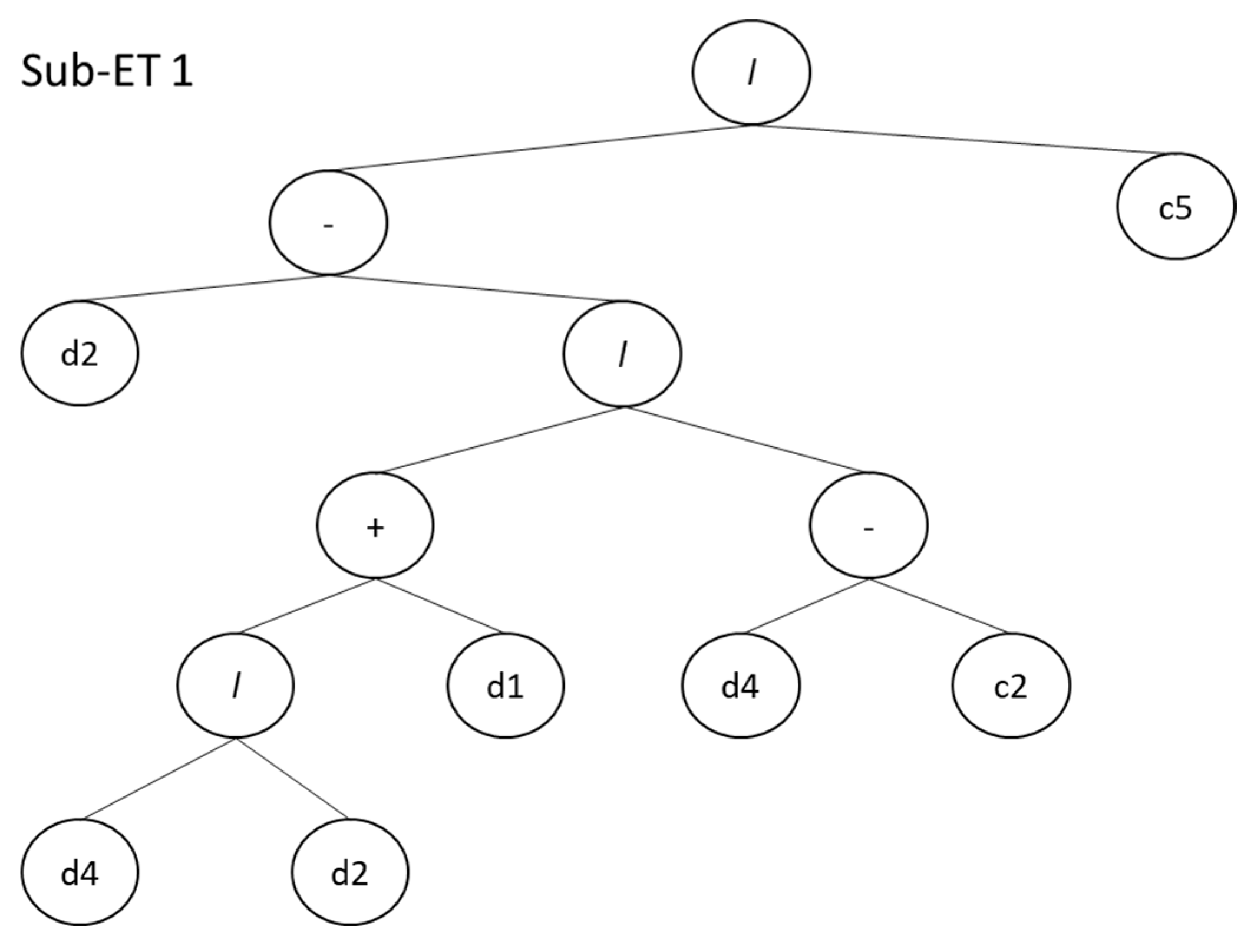
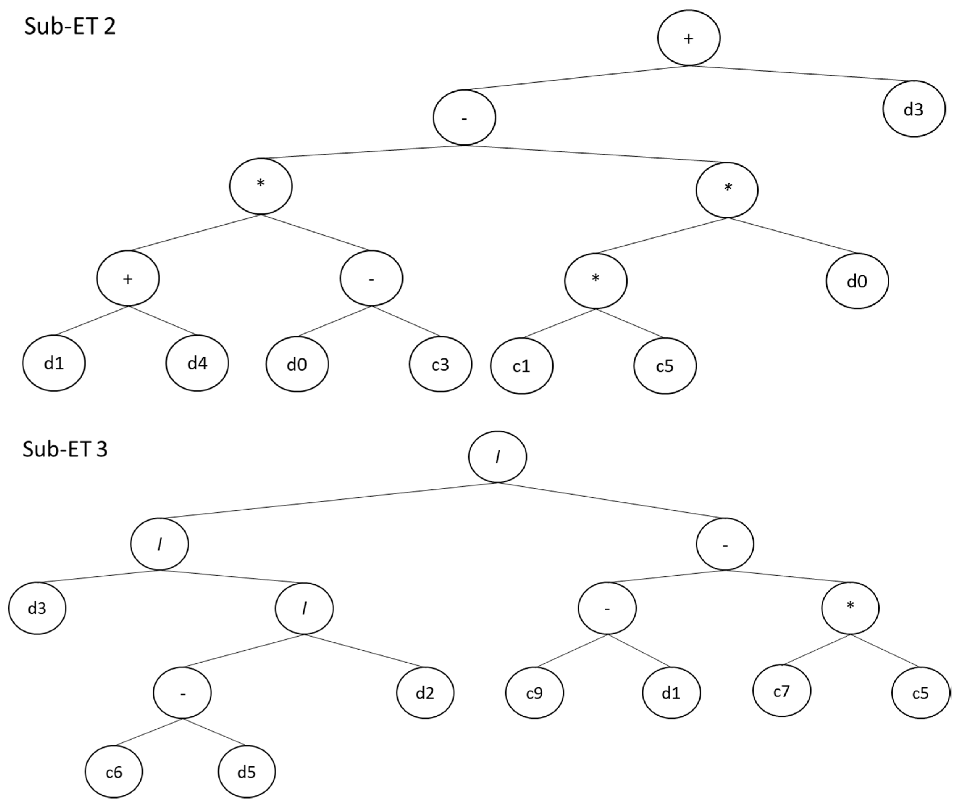
| Parameters Notation | Parameters | Constant Notations | Constant Values |
|---|---|---|---|
| d0 | Cement | G1C5 | −4.28835075 |
| d1 | Fly ash | G1C2 | 37.75001621 |
| d2 | Water–powder | G2C3 | 39.89209066 |
| d3 | Fine aggregate | G2C1 | 9.967413128 |
| d4 | Coarse aggregate | G2C5 | 26.22055325 |
| d5 | Superplasticizer | G3C9 | −20.52776364 |
| - | - | G3C7 | 145.5520044 |
| - | - | G3C5 | −10.5395382 |
| - | - | G3C6 | 544.4511609 |
Publisher’s Note: MDPI stays neutral with regard to jurisdictional claims in published maps and institutional affiliations. |
© 2021 by the authors. Licensee MDPI, Basel, Switzerland. This article is an open access article distributed under the terms and conditions of the Creative Commons Attribution (CC BY) license (https://creativecommons.org/licenses/by/4.0/).
Share and Cite
Farooq, F.; Czarnecki, S.; Niewiadomski, P.; Aslam, F.; Alabduljabbar, H.; Ostrowski, K.A.; Śliwa-Wieczorek, K.; Nowobilski, T.; Malazdrewicz, S. A Comparative Study for the Prediction of the Compressive Strength of Self-Compacting Concrete Modified with Fly Ash. Materials 2021, 14, 4934. https://doi.org/10.3390/ma14174934
Farooq F, Czarnecki S, Niewiadomski P, Aslam F, Alabduljabbar H, Ostrowski KA, Śliwa-Wieczorek K, Nowobilski T, Malazdrewicz S. A Comparative Study for the Prediction of the Compressive Strength of Self-Compacting Concrete Modified with Fly Ash. Materials. 2021; 14(17):4934. https://doi.org/10.3390/ma14174934
Chicago/Turabian StyleFarooq, Furqan, Slawomir Czarnecki, Pawel Niewiadomski, Fahid Aslam, Hisham Alabduljabbar, Krzysztof Adam Ostrowski, Klaudia Śliwa-Wieczorek, Tomasz Nowobilski, and Seweryn Malazdrewicz. 2021. "A Comparative Study for the Prediction of the Compressive Strength of Self-Compacting Concrete Modified with Fly Ash" Materials 14, no. 17: 4934. https://doi.org/10.3390/ma14174934
APA StyleFarooq, F., Czarnecki, S., Niewiadomski, P., Aslam, F., Alabduljabbar, H., Ostrowski, K. A., Śliwa-Wieczorek, K., Nowobilski, T., & Malazdrewicz, S. (2021). A Comparative Study for the Prediction of the Compressive Strength of Self-Compacting Concrete Modified with Fly Ash. Materials, 14(17), 4934. https://doi.org/10.3390/ma14174934