
Key Factors for Implementing Magnetic NDT Method on Thin UHPFRC Bridge Elements


Abstract
:1. Introduction
2. Non-Destructive Method
2.1. Principles
2.2. Determination of Fibre Content and Fibre Orientation
2.2.1. Fibre Content
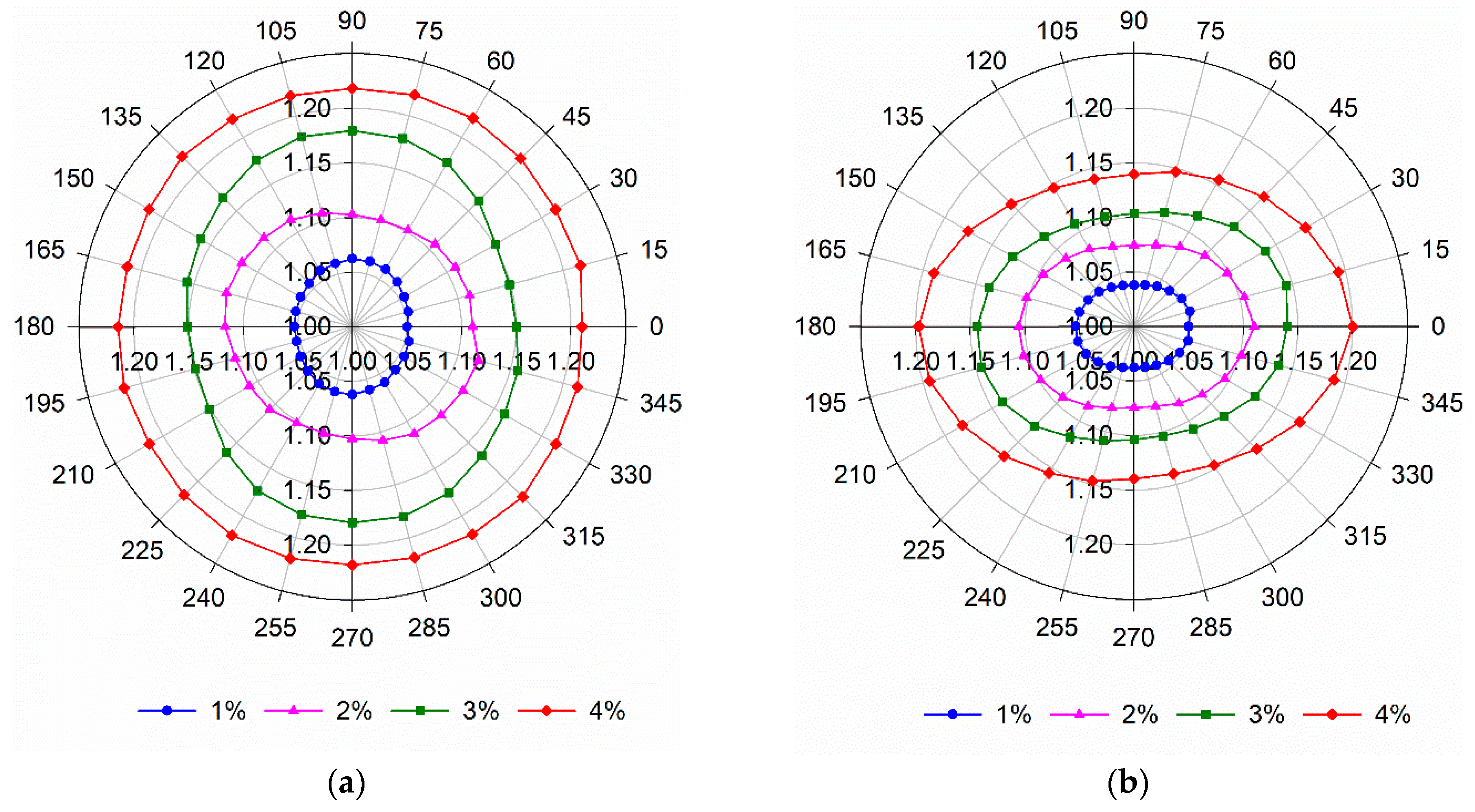
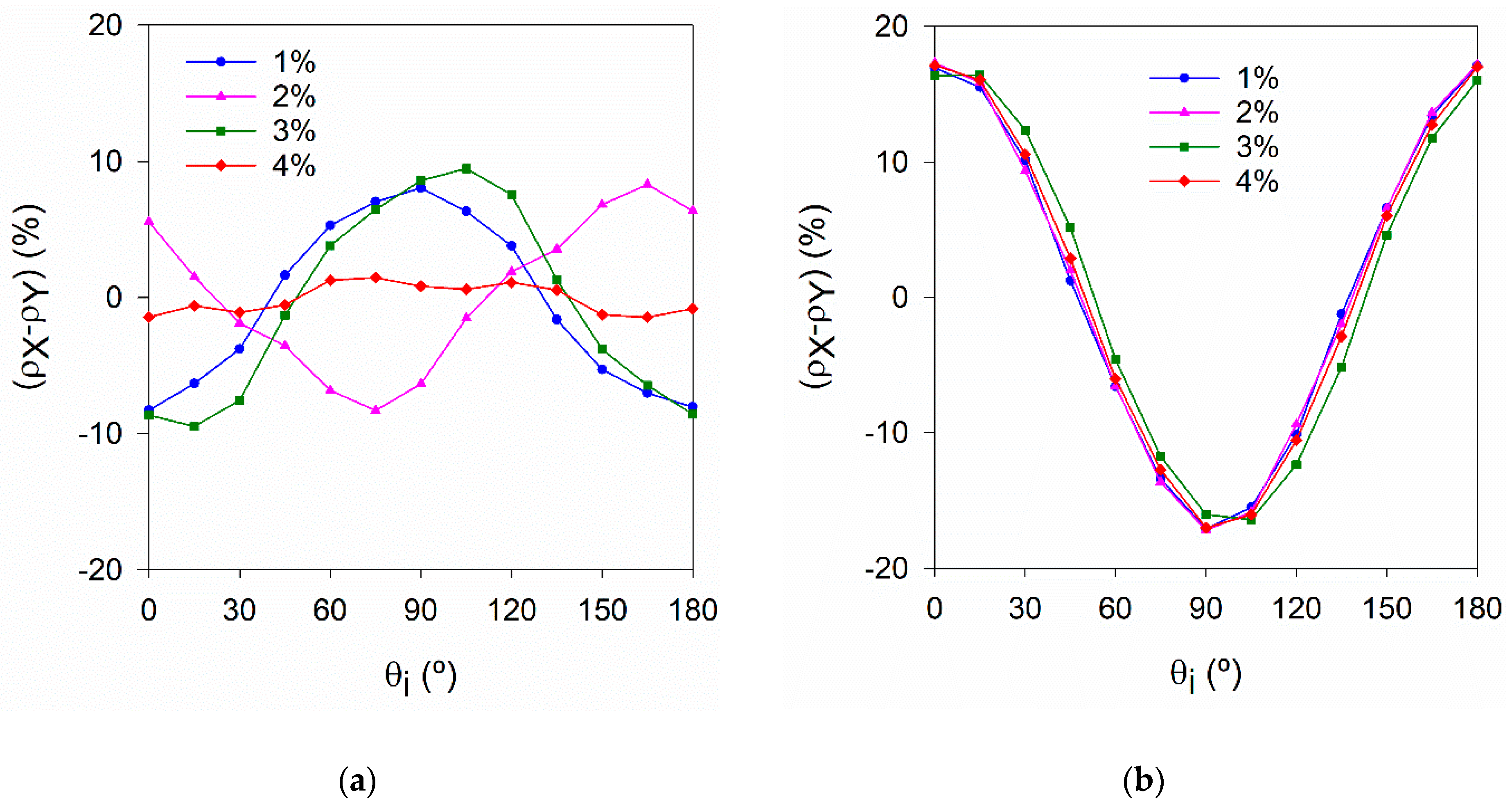
2.2.2. Fibre Orientation
2.3. Estimation of the (Post-Cracking) Tensile Strength
3. Experimental Programme
3.1. Materials and Mix-Proportions
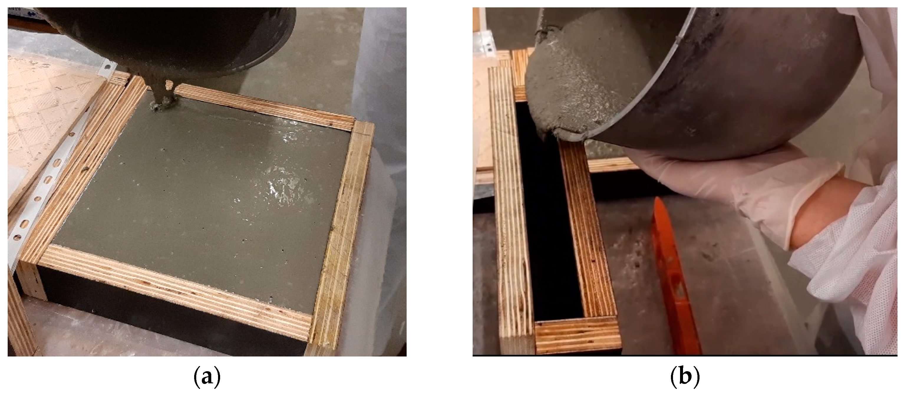
3.2. Mixing, Workability and Specimen Preparation
3.3. NDT Testing
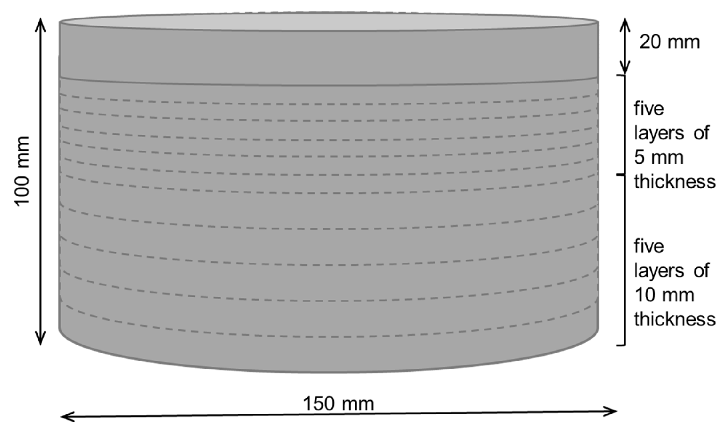
3.3.1. Test Series A
3.3.2. Test Series B
3.3.3. Test Series C
4. Results and Discussion
4.1. Workability
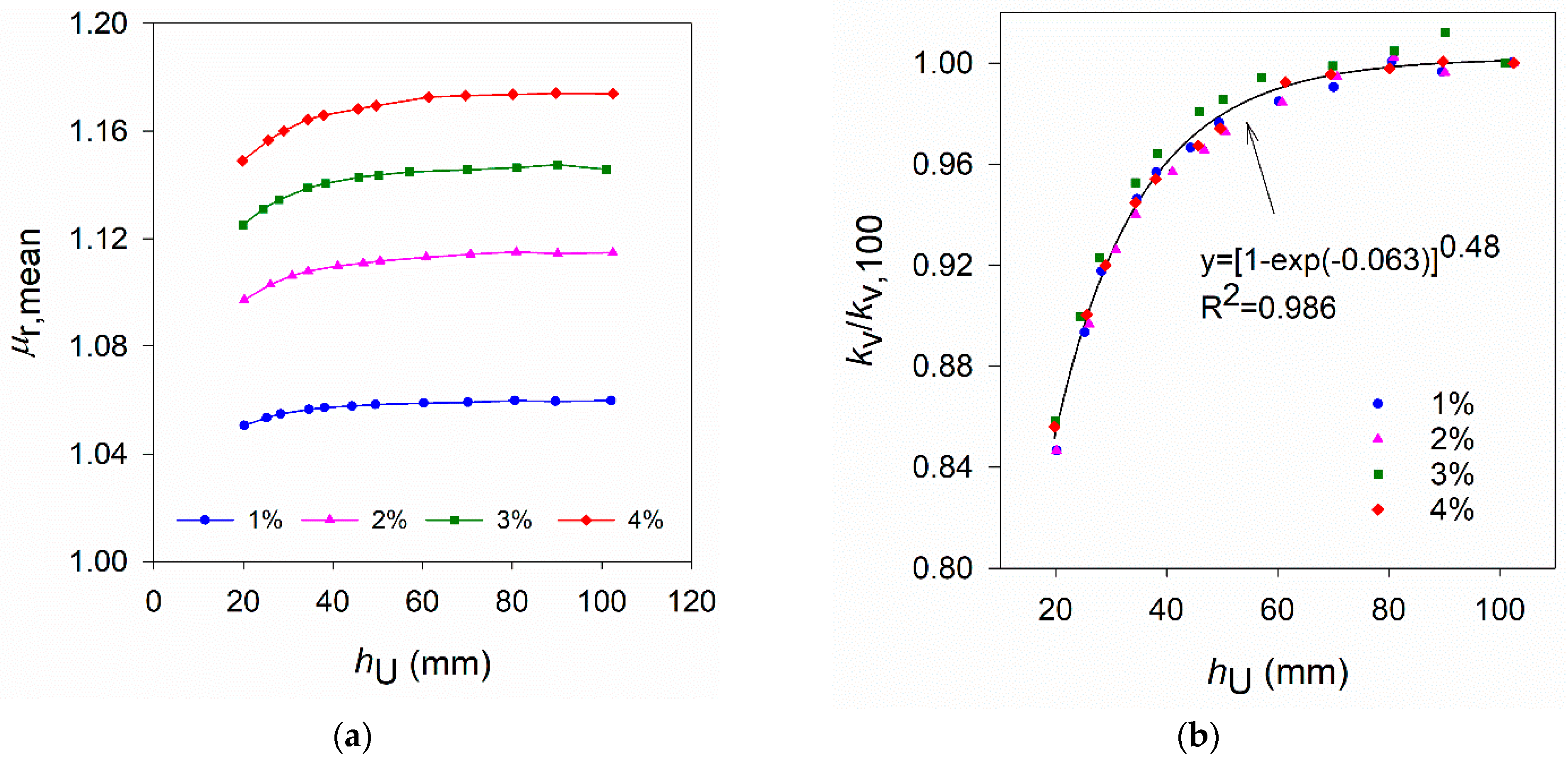
4.2. Effect of Specimen Thickness
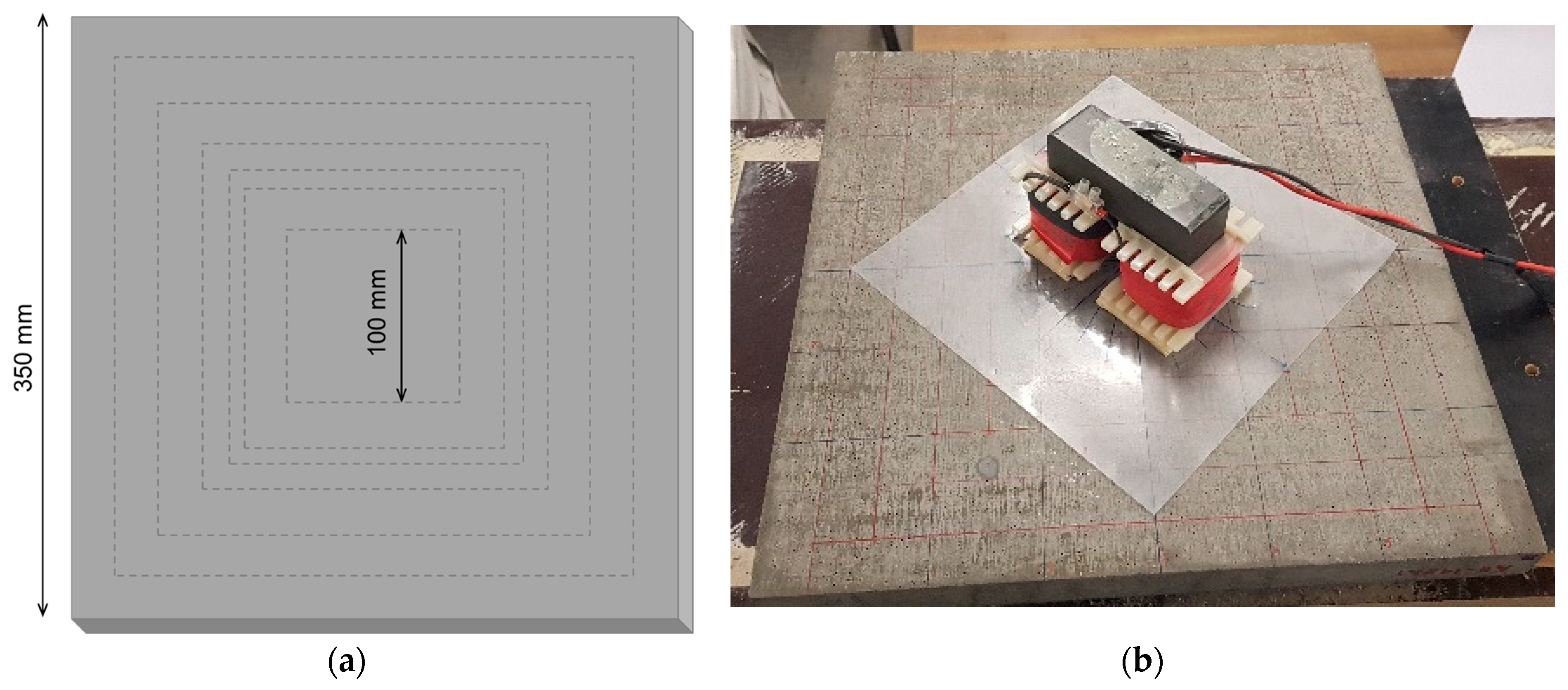
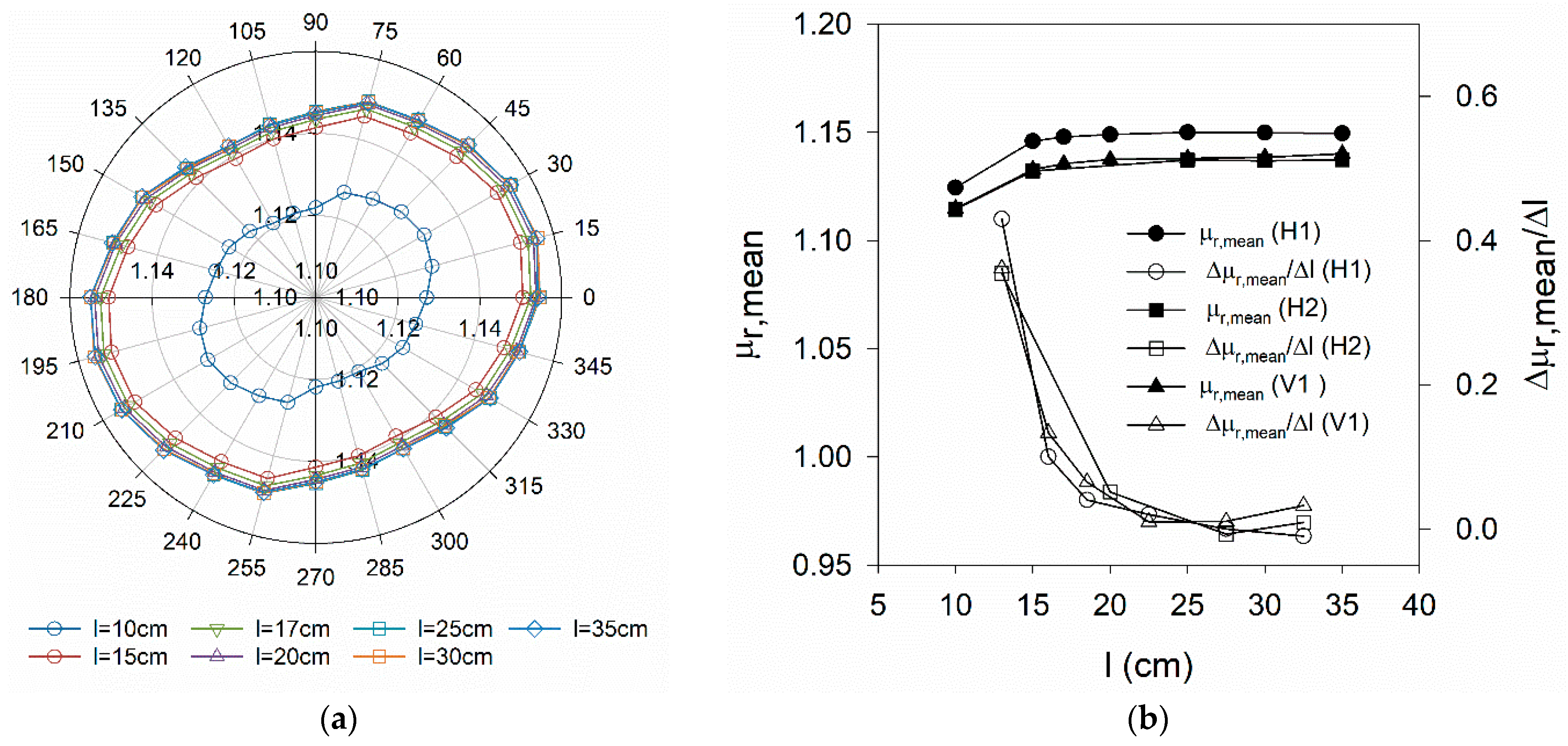
4.3. Effect of the Specimen Area
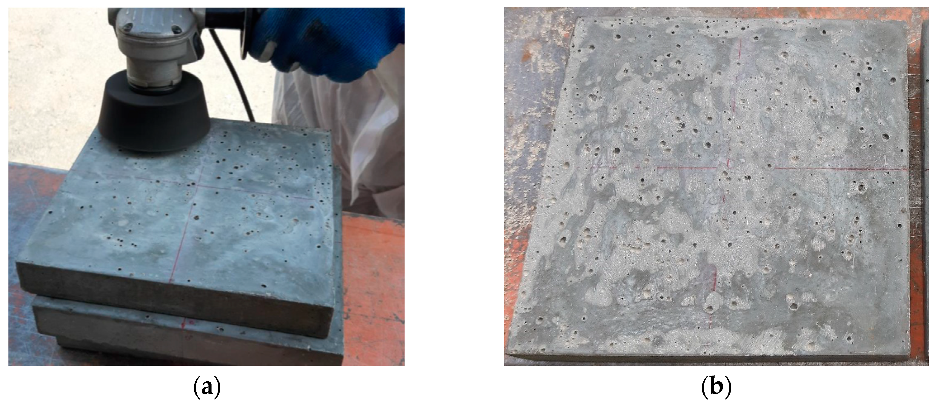
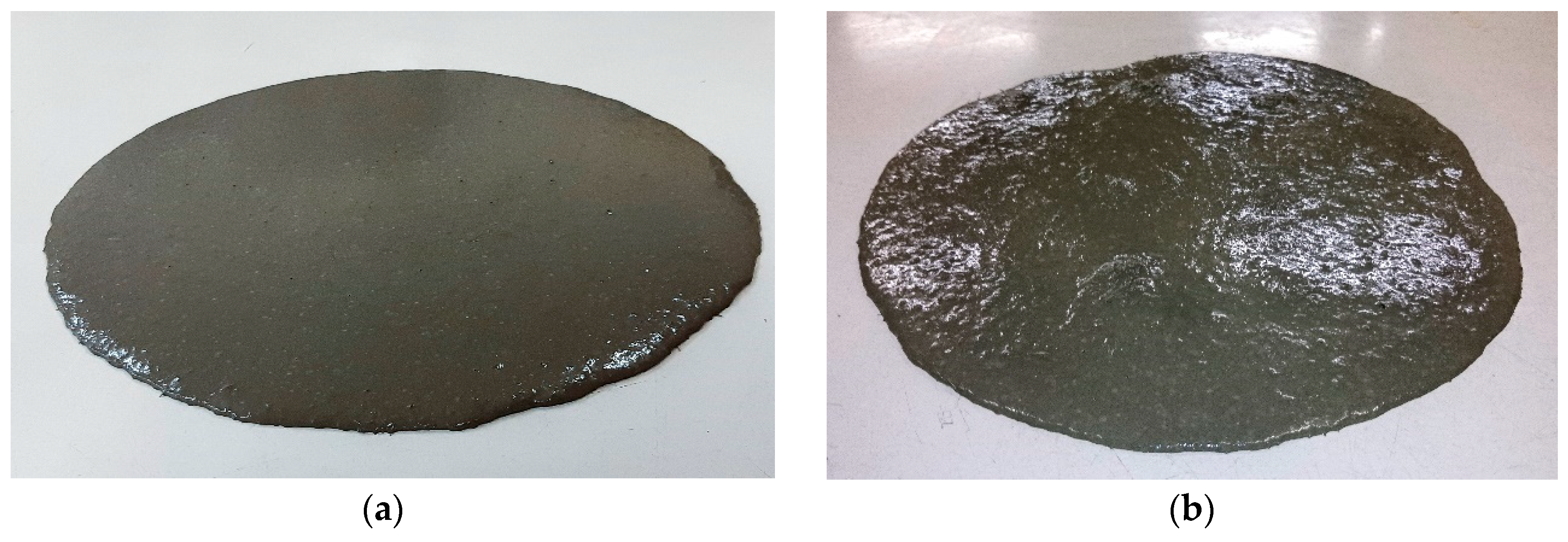
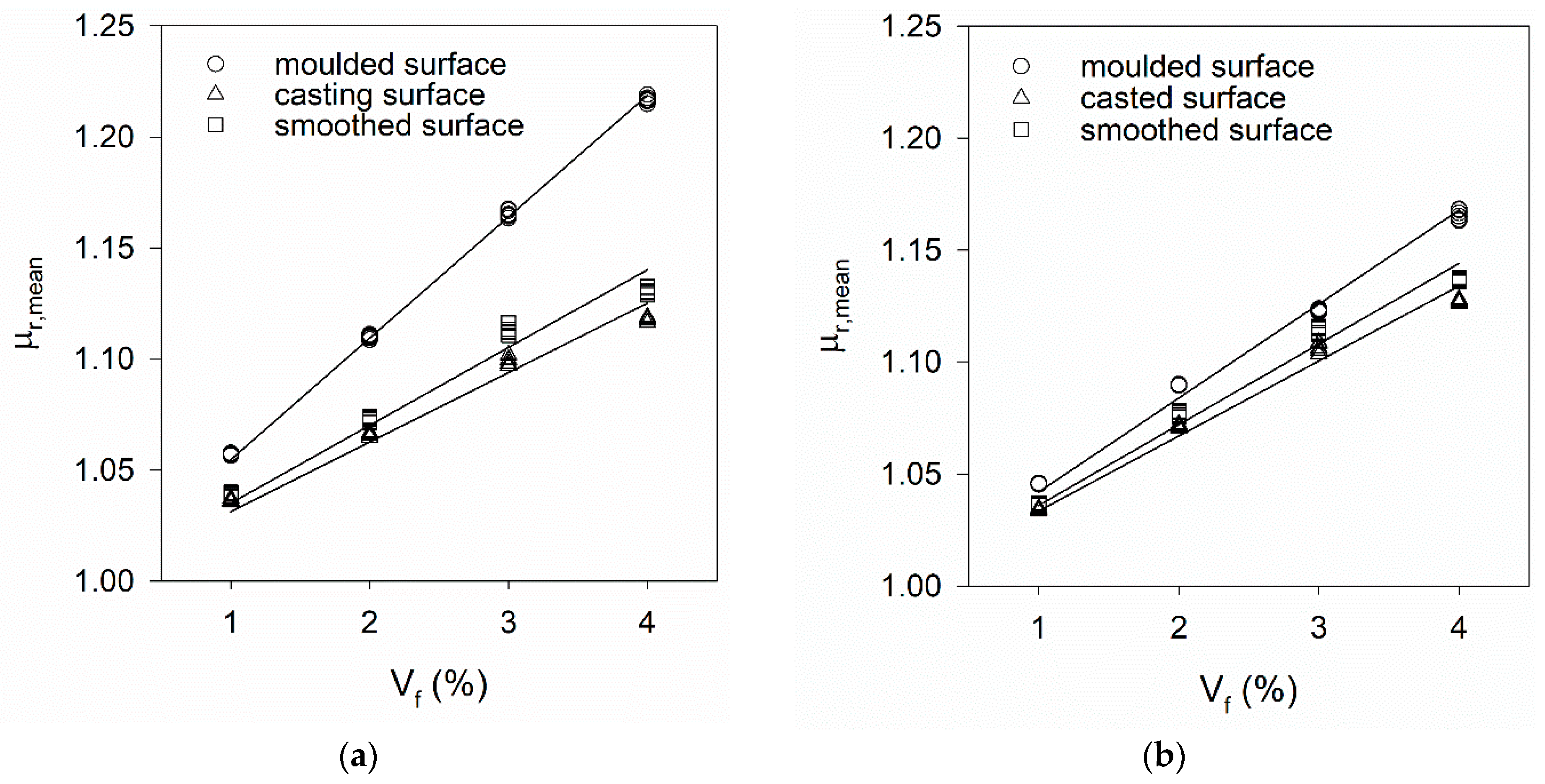
4.4. Effect of Surface Roughness
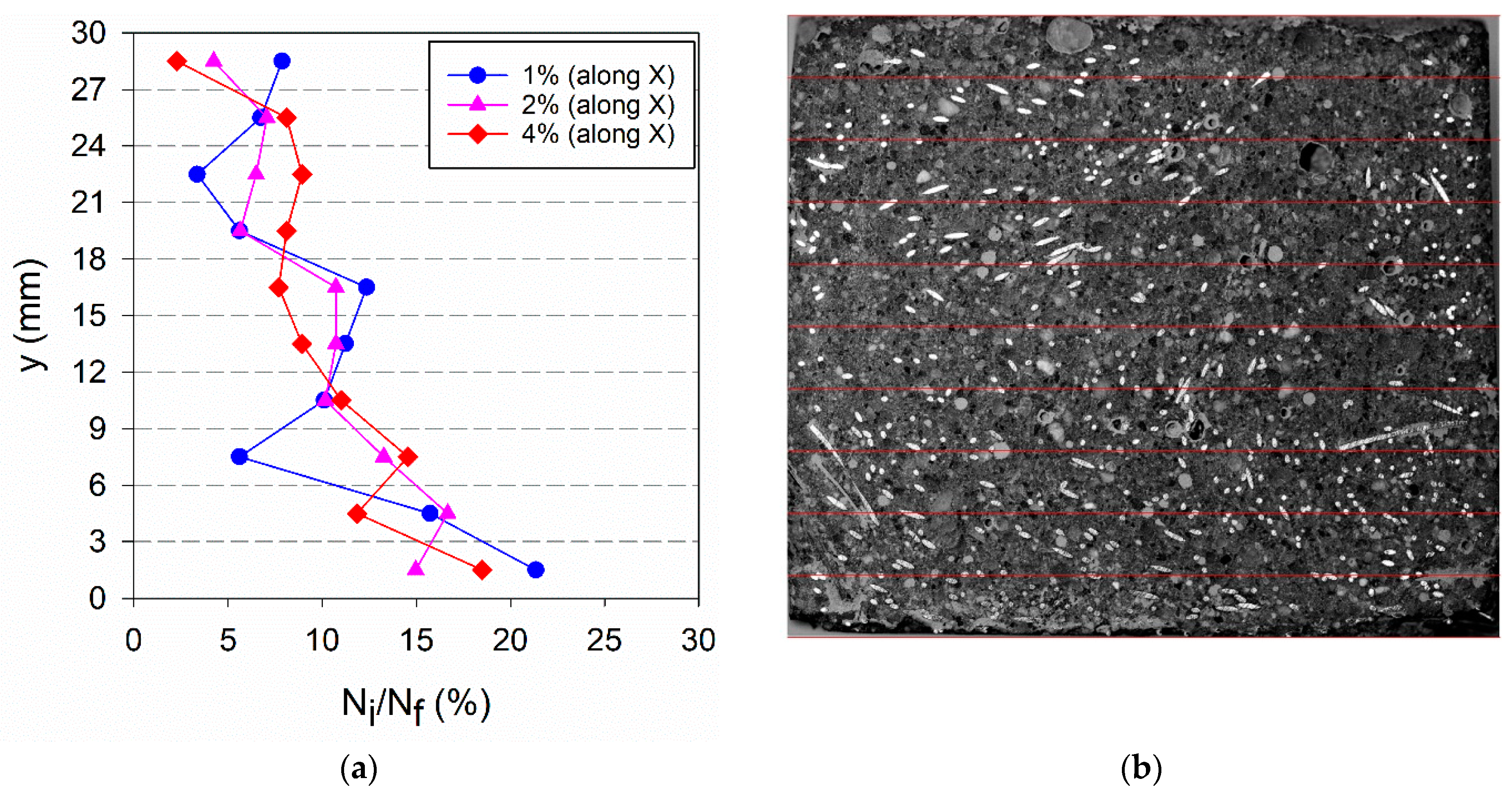
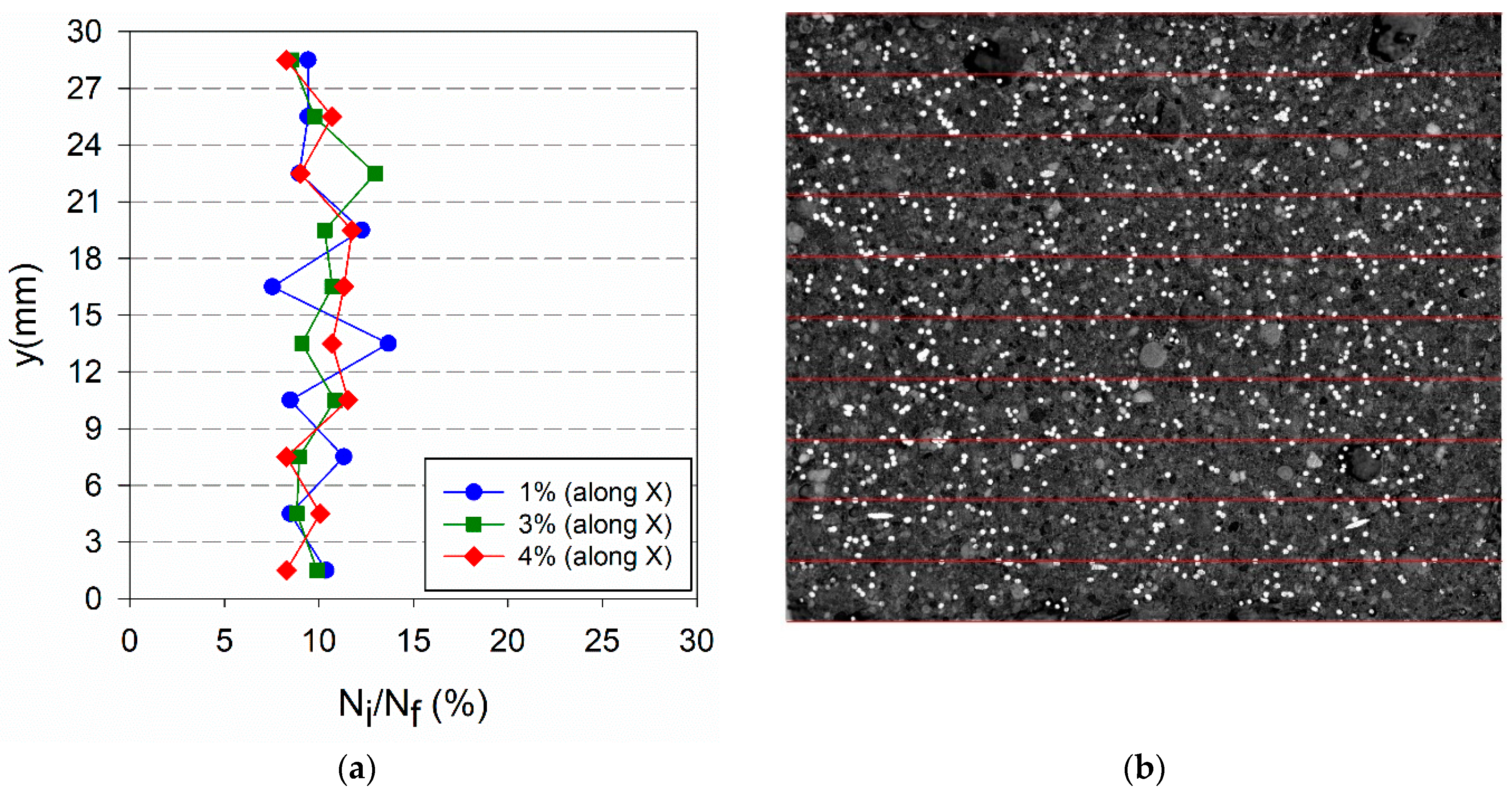
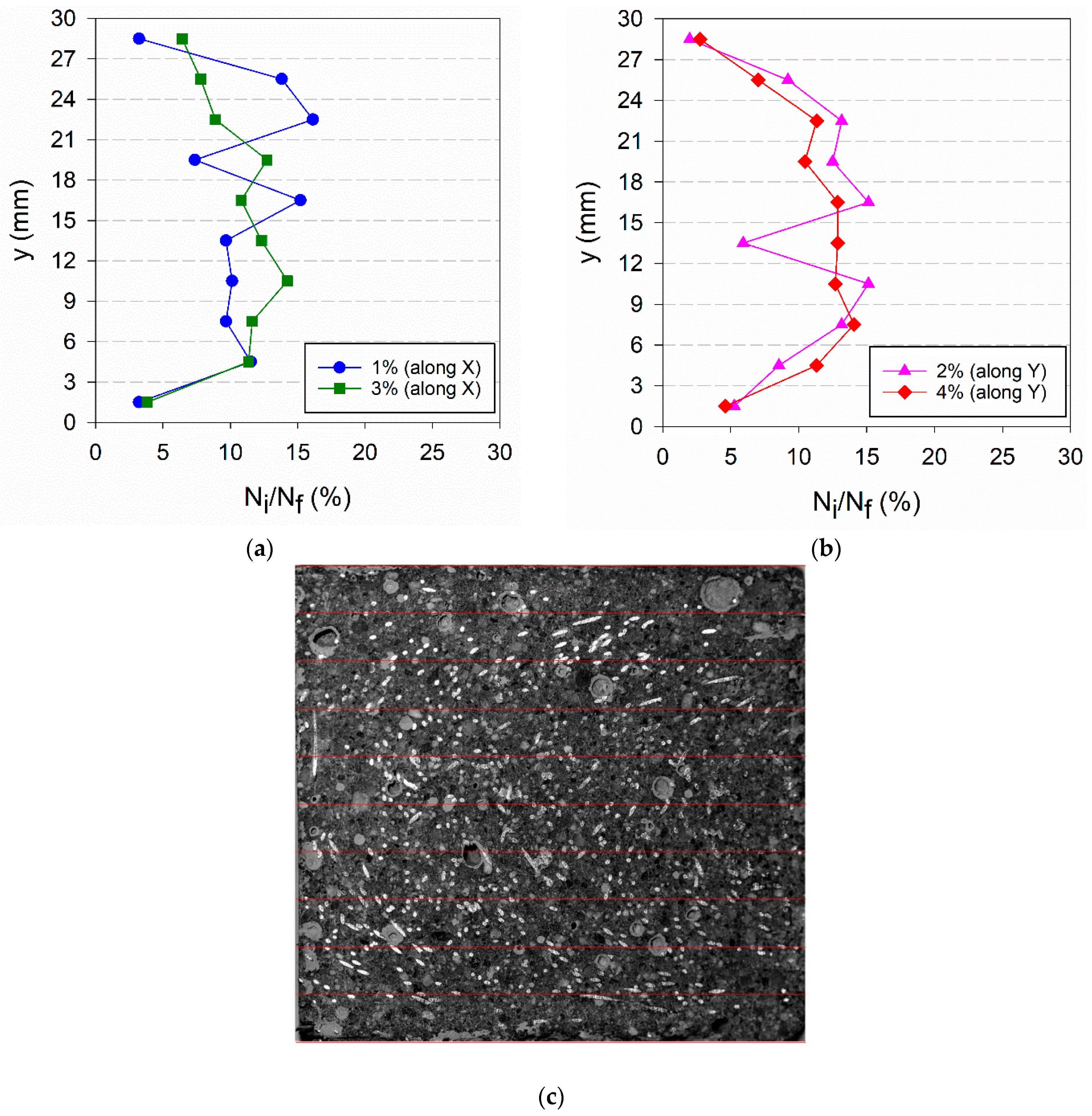
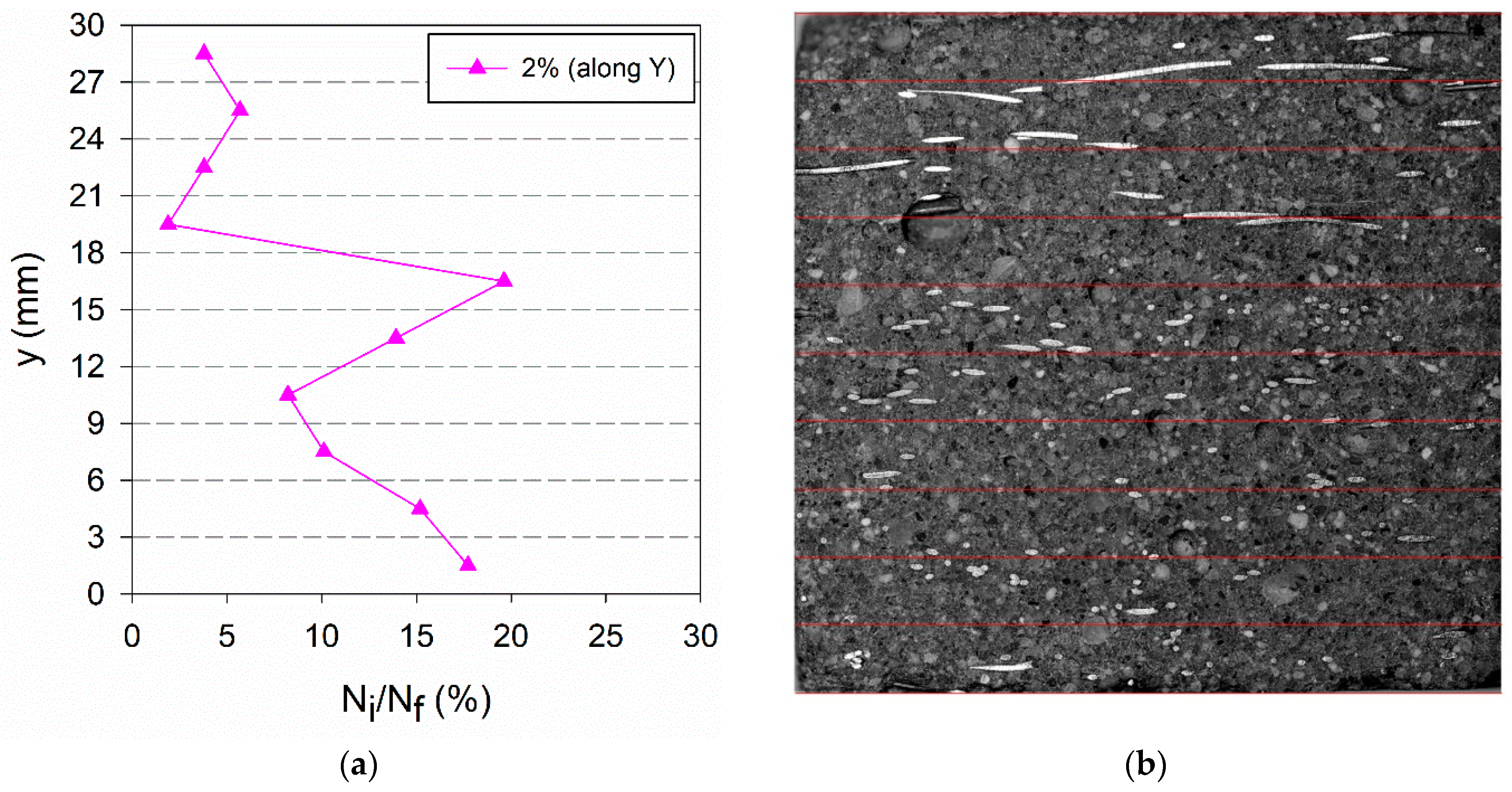
4.5. Effect of Fibres Segregation (In-Depth)
5. Conclusions
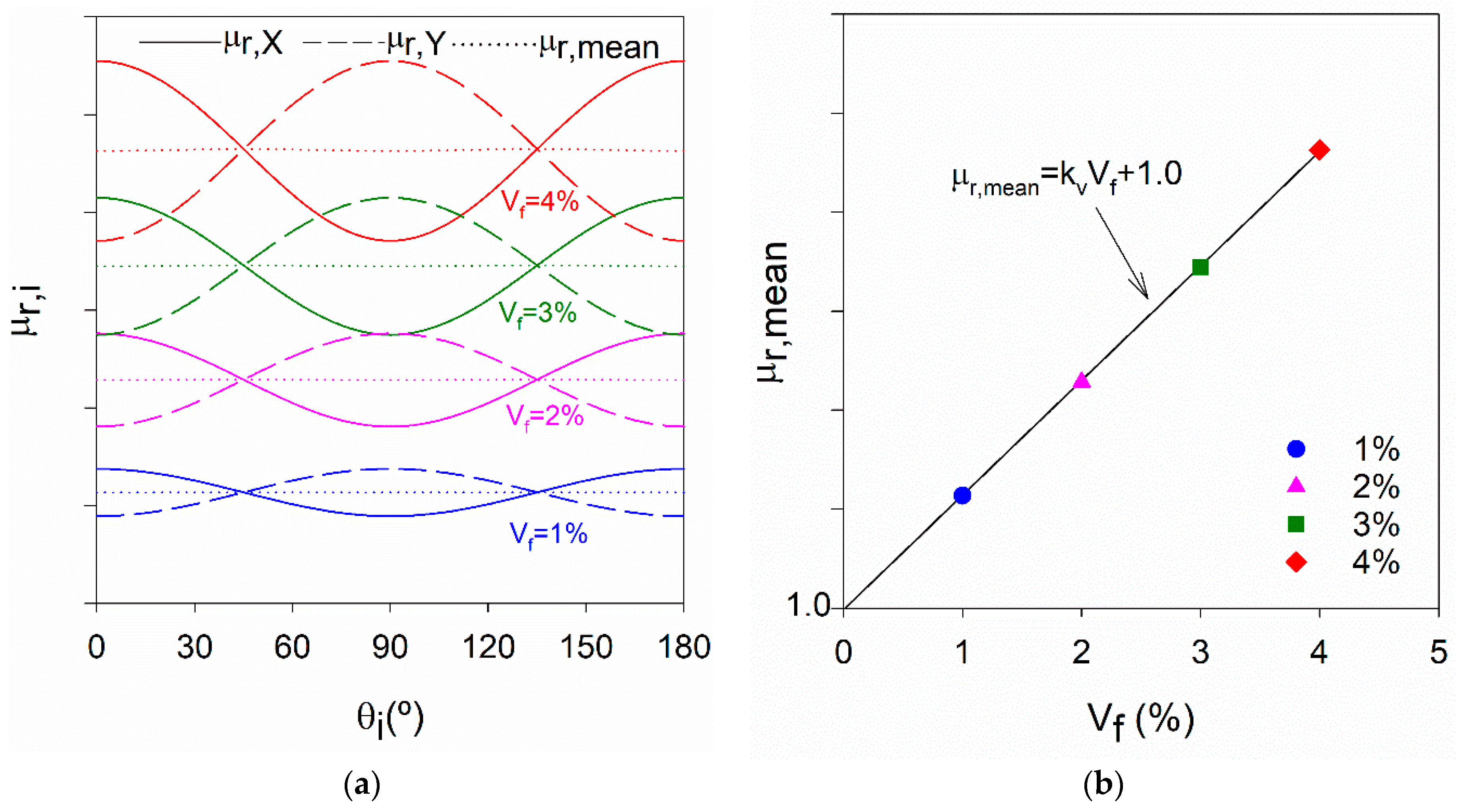
- The proportionality constant that allows to predict Vf from the μr,mean estimated using the magnetic probe changes with the thickness of the UHPFRC layer (hU). A correction function is proposed for as a function of hU.
- The magnetic probe used in this study is capable of evaluating the fibre content and fibre orientation in the UHPFRC up to a depth of 70 mm measured from the contact surface. In UHPFRC elements where it is possible to take measurements on two opposite sides the assessed material thickness can be doubled.
- To perform measurements with a probe similar to the one used in this study, the measuring points (the point at which the probe is centred) are recommended to be at a minimum distance of 100 mm from the sides of the test specimens/elements.
- The probe measurements should be performed preferably over a moulded and smooth surface since perfect contact between the probe and the UHPFRC material is necessary to obtain representative measurements. Unevenness, for example, in the casting surfaces, should be removed by grinding.
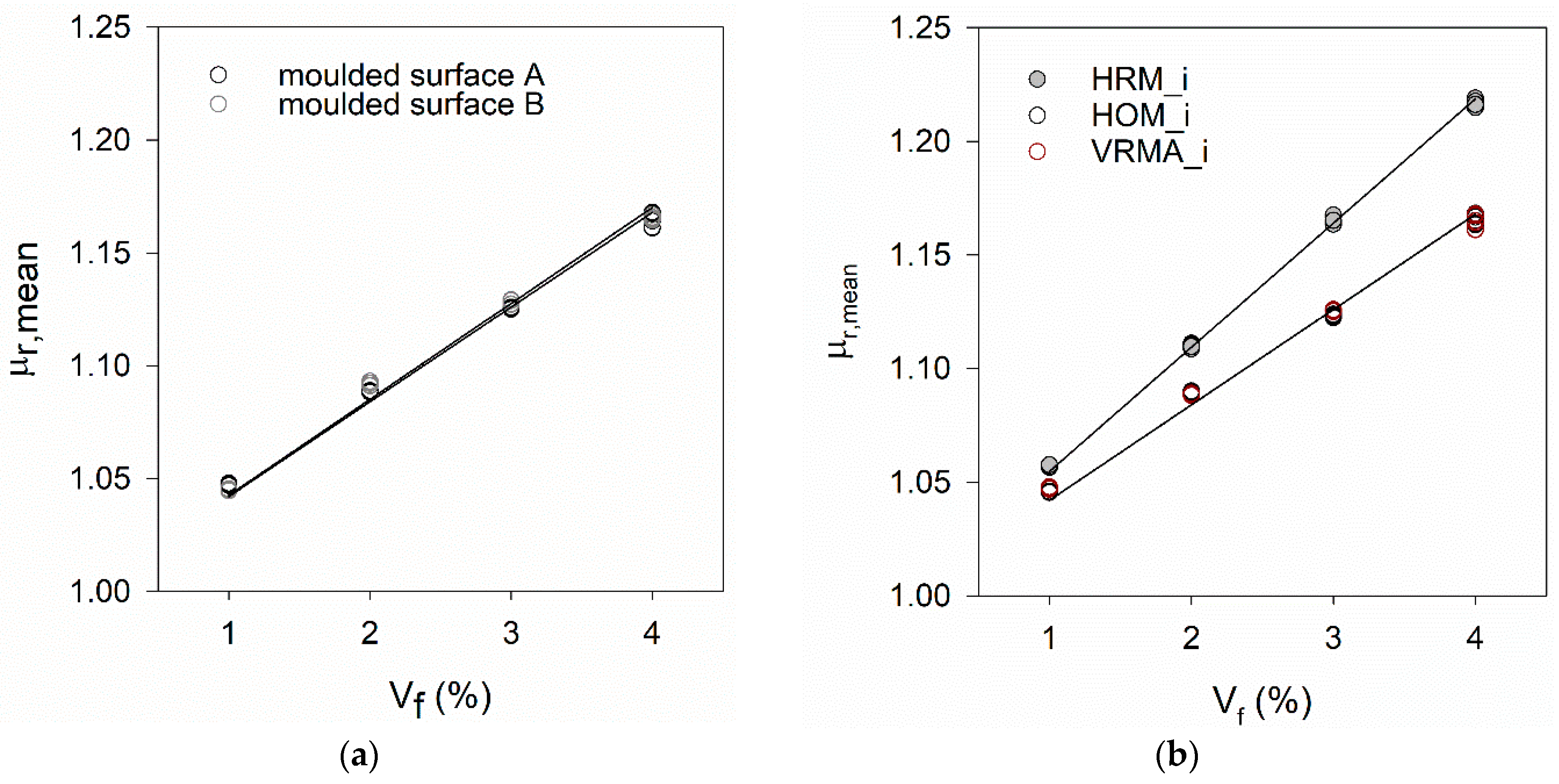
- The magnetic probe is sensitive to the occurrence of in-depth fibres segregation. Even in thin UHPFRC layers, fibres settlement can occur when casting with more fluid mixtures due to gravity action and/or when the material is agitated during casting.
Author Contributions
Funding
Institutional Review Board Statement
Informed Consent Statement
Acknowledgments
Conflicts of Interest
References
- Graybeal, B.; Brühwiler, E.; Kim, B.-S.; Toutlemonde, F.; Voo, Y.L.; Zaghi, A. International Perspective on UHPC in Bridge Engineering. J. Bridge Eng. 2020, 25, 04020094. [Google Scholar] [CrossRef]
- Toutlemonde, F.; Bernadi, S.; Brugeaud, Y.; Simon, A. Twenty Years-Long French Experience in UHPFRC Application and Paths Opened from the Completion of the Standards for UHPFRC. 2018. Available online: https://hal.archives-ouvertes.fr/hal-01955204 (accessed on 26 July 2021).
- Marek, J.; Kolisko, J.; Tej, P.; Čítek, D.; Komanec, J.; Kalný, M.; Vráblík, L. New UHPFRC bridges in the Czech Republic. IOP Conf. Ser. Mater. Sci. Eng. 2019, 596. [Google Scholar] [CrossRef]
- López, J.Á.; Serna, P.; Navarro-Gregori, J.; Camacho, E. Construction of the U-Shaped Truss Footbridge over the Ovejas Ravine in Alicante. In Proceedings of the 2º International Symposium on UHPFRC. Designing and Building with UHPFRC, Marseille France, 1–3 October 2013. [Google Scholar]
- Brühwiler, E.; Denarié, E. Rehabilitation and Strengthening of Concrete Structures Using Ultra-High Performance Fibre Reinforced Concrete. Struct. Eng. Int. 2013, 23, 450–457. [Google Scholar] [CrossRef]
- Alberti, M.G.; Enfedaque, A.; Galvez, J. A review on the assessment and prediction of the orientation and distribution of fibres for concrete. Compos. Part. B Eng. 2018, 151, 274–290. [Google Scholar] [CrossRef]
- Huang, H.; Gao, X.; Teng, L. Fiber alignment and its effect on mechanical properties of UHPC: An overview. Constr. Build. Mater. 2021, 296, 123741. [Google Scholar] [CrossRef]
- Pastor, F.; Hajar, Z.; Palu, P.D. UHPFRC Footbridge in le CANNET des MAURES. In Proceedings of the AFGC-ACI-fib-RILEM Int. Symposium on Ultra-High Performance Fibre-Reinforced Concrete, UHPFRC, Montpellier, France, 2–4 October 2017. [Google Scholar]
- Brühwiler, E.; Bastien-Masse, M.; Mühlberg, H.; Houriet, B.; Fleury, B.; Cuennet, S.; Schär, P.; Boudry, F.; Maurer, M. Strengthening the Chillon viaducts deck slabs with reinforced UHPFRC. In Proceedings of the IABSE Conference Geneva 2015 ‘Structural Engineering: Providing Solutions to Global Challenges’, Geneva, Switzerland, 23–25 September 2015. [Google Scholar] [CrossRef] [Green Version]
- Bastien-Masse, M.; Denarié, E.; Brühwiler, E. Effect of fiber orientation on the in-plane tensile response of UHPFRC reinforcement layers. Cem. Concr. Compos. 2016, 67, 111–125. [Google Scholar] [CrossRef]
- Abrishambaf, A.; Pimentel, M.; Nunes, S. Influence of fibre orientation on the tensile behaviour of ultra-high performance fibre reinforced cementitious composites. Cem. Concr. Res. 2017, 97, 28–40. [Google Scholar] [CrossRef]
- Shen, X.; Brühwiler, E. Influence of local fiber distribution on tensile behavior of strain hardening UHPFRC using NDT and DIC. Cem. Concr. Res. 2020, 132, 106042. [Google Scholar] [CrossRef]
- Miletić, M.; Kumar, L.M.; Arns, J.-Y.; Agarwal, A.; Foster, S.; Arns, C.; Perić, D. Gradient-based fibre detection method on 3D micro-CT tomographic image for defining fibre orientation bias in ultra-high-performance concrete. Cem. Concr. Res. 2020, 129, 105962. [Google Scholar] [CrossRef]
- Krause, M.S.; Hausherr, J.M.; Burgeth, B.; Herrmann, C.; Krenkel, W. Determination of the fibre orientation in composites using the structure tensor and local X-ray transform. J. Mater. Sci. 2010, 45, 888–896. [Google Scholar] [CrossRef]
- Ferrara, L.; Faifer, M.; Toscani, S. A magnetic method for non destructive monitoring of fiber dispersion and orientation in steel fiber reinforced cementitious composites—Part 1: Method calibration. Mater. Struct. 2011, 45, 575–589. [Google Scholar] [CrossRef]
- Ferrara, L.; Faifer, M.; Muhaxheri, M.; Toscani, S. A magnetic method for non destructive monitoring of fiber dispersion and orientation in steel fiber reinforced cementitious composites. Part 2: Correlation to tensile fracture toughness. Mater. Struct. 2011, 45, 591–598. [Google Scholar] [CrossRef]
- Cavalaro, S.H.P.; López-Carreño, R.; Torrents, J.M.; Aguado, A.; Juan-García, P. Assessment of fibre content and 3D profile in cylindrical SFRC specimens. Mater. Struct. 2015, 49, 577–595. [Google Scholar] [CrossRef] [Green Version]
- Nunes, S.; Pimentel, M.; Carvalho, A. Non-destructive assessment of fibre content and orientation in UHPFRC layers based on a magnetic method. Cem. Concr. Compos. 2016, 72, 66–79. [Google Scholar] [CrossRef]
- Ozyurt, N.; Mason, T.O.; Shah, S.P. Non-destructive monitoring of fiber orientation using AC-IS: An industrial-scale application. Cem. Concr. Res. 2006, 36, 1653–1660. [Google Scholar] [CrossRef]
- Lataste, J.; Behloul, M.; Breysse, D. Characterisation of fibres distribution in a steel fibre reinforced concrete with electrical resistivity measurements. NDT E Int. 2008, 41, 638–647. [Google Scholar] [CrossRef]
- Nunes, S.; Pimentel, M.; Ribeiro, F.; Milheiro-Oliveira, P.; Carvalho, A. Estimation of the tensile strength of UHPFRC layers based on non-destructive assessment of the fibre content and orientation. Cem. Concr. Compos. 2017, 83, 222–238. [Google Scholar] [CrossRef] [Green Version]
- Li, L.; Xia, J.; Chin, C.; Jones, S. Fibre Distribution Characterization of Ultra-High Performance Fibre-Reinforced Concrete (UHPFRC) Plates using Magnetic Probes. Materials 2020, 13, 5064. [Google Scholar] [CrossRef]
- Li, L.; Xia, J.; Galobardes, I. Magnetic probe to test spatial distribution of steel fibres in UHPFRC prisms. In Proceedings of the 5th International fib Congress: Better-Smarter-Stronger, Melbourne, Australia, 7–11 October 2018. [Google Scholar]
- Nunes, S.; Ribeiro, F.; Carvalho, A.; Pimentel, M.; Brühwiler, E.; Bastien-Masse, M. Non-destructive measurements to evaluate fiber dispersion and content in UHPFRC reinforcement layers. In Proceedings of the Multi-Span Large Bridges Conference, Porto, Portugal, 1–3 July 2015. [Google Scholar]
- Davis, J.; Huang, Y.; Millard, S.G.; Bungey, J. Determination of Dielectric Properties of Insitu Concrete at Radar Frequencies. Non-Destr. Test. Civ. Eng. 2003. Available online: https://www.ndt.net/article/ndtce03/papers/v078/v078.htm (accessed on 23 July 2021).
- Sine, A.G. Strengthening of Reinforced Concrete Elements with UHPFRC; Faculty of Civil Engineering, Porto University: Porto, Portugal, 2021. [Google Scholar]
- Krenchel, H. Fibre spacing and specific fibre surface. In Fibre Reinforced Cement and Concrete; Construction Press: London, UK, 1975; pp. 69–79. [Google Scholar]
- Abrishambaf, A.; Pimentel, M.; Nunes, S. A meso-mechanical model to simulate the tensile behaviour of ultra-high performance fibre-reinforced cementitious composites. Compos. Struct. 2019, 222, 110911. [Google Scholar] [CrossRef]
- BIBM; Cembureau; ERMCO; EFCA; EFNARC. The European Guidelines for Self-Compacting Concrete Specification, Production and Use. 2005. Available online: https://www.theconcreteinitiative.eu/images/ECP_Documents/EuropeanGuidelinesSelfCompactingConcrete.pdf (accessed on 2 August 2021).
- Wang, R.; Gao, X.; Huang, H.; Han, G. Influence of rheological properties of cement mortar on steel fiber distribution in UHPC. Constr. Build. Mater. 2017, 144, 65–73. [Google Scholar] [CrossRef]
- Rasband, W.S. ImageJ; U.S. National Institutes of Health: Bethesda, MD, USA. Available online: https://imagej.nih.gov/ij/ (accessed on 26 July 2021).

| U-Shape Ferrite Core | Copper Wire Coil | ||||
|---|---|---|---|---|---|
| Reference | Relative Magnetic Permeability | Length | Cross-Section | Wire Diameter | Number of Turns |
| Siemens ferrite N47 | ~2000 | 189 mm | 28 × 30 mm2 | 0.5 mm | 1454 |
| UHPFRC | Constituent Materials | Vf = 1% | Vf = 2% | Vf = 3% | Vf = 4% |
|---|---|---|---|---|---|
| Cementitious matrix | Cement | 794.9 | |||
| Silica fume | 79.49 | ||||
| Limestone filler | 311.43 | ||||
| Water | 145.36 | ||||
| Superplasticizer | 30 | ||||
| Sp/c * | 1.51% | ||||
| Sand | 993.56 | 967.26 | 940.96 | 914.66 | |
| Steel fibres (straight) | lf = 9 mm/df = 0.175 mm | 39.25 | 78.5 | 117.5 | 157 |
| lf = 12 mm/df = 0.175 mm | 39.25 | 78.5 | 117.5 | 157 | |
| Test Series: | A | B | C | |
|---|---|---|---|---|
| Effect Being Evaluated: | Thickness | Area | Surface Roughness | Fibres Segregation (In-Depth) |
| specimen’s | cylinder | square plate | square plate | |
| geometry | h = 100 to 20 mm | l = 350 to 100 mm | l = 200 mm | |
| ϕ = 150 mm | h = 30 mm | h = 30 mm | ||
| total fibre content | 1% | 3% | 1% | |
| 2% | 2% | |||
| 3% | 3% | |||
| 4% | 4% | |||
| number of specimens | 4 | 3 | 12 | |
| fibres orientation | random | random | random | |
| oriented * | ||||
| mould position | horizontal | horizontal | horizontal | |
| vertical | vertical | |||
| condition of the test surface | moulded | moulded | moulded surface | |
| casting surface | ||||
| polished surface | ||||
| Mould Position | Fibres Orientation | Condition of the Test Surface | Specimens Reference * | |
|---|---|---|---|---|
| Horizontal | Random | Moulded surface | HRM_i | HR_i |
| Casting surface | HRC_i | |||
| Smoothed surface | HRS_i | |||
| Horizontal | Oriented | Moulded surface | HOM_i | HO_i |
| Casting surface | HOC_i | |||
| Smoothed surface | HOS_i | |||
| Vertical | Random | Moulded surface A | VRMA_i | VR_i |
| Moulded surface B | VRMB_i | |||
| Test Series | Casting Date | Reference | Vf = 1% | Vf = 2% | Vf = 3% | Vf = 4% |
|---|---|---|---|---|---|---|
| A | 22 May 2019 | -- | 294.5 | 295.0 | 291.5 | 263.0 |
| C | 12 June 2019 | HR_i | 295.5 | 289.0 | 287.5 | 281.0 |
| or | HO_i | 286.0 | 287.5 | 284.0 | 280.5 | |
| 14 June 2019 | VR_i | 288.5 | 287.0 | 288.0 | 274.0 | |
| Average | 290.0 | 289.6 | 287.8 | 274.6 | ||
| Standard deviation | 4.9 | 3.7 | 3.1 | 8.4 | ||
| Coefficient of variation | 1.7% | 1.3% | 1.1% | 3.1% | ||
| Mould Position | Fibres Orientation | Reference | kV | R2 |
|---|---|---|---|---|
| Horizontal | Random | HRM_i | 5.5 | 0.999 |
| HRC_i | 3.1 | 0.965 | ||
| HRS_i | 3.5 | 0.965 | ||
| Oriented | HOM_i | 4.2 | 0.992 | |
| HOC_i | 3.4 | 0.980 | ||
| HOS_i | 3.6 | 0.979 | ||
| Vertical | Random | VRMA_i | 4.2 | 0.991 |
| VRMB_i | 4.3 | 0.990 |
| Fibre Content | HR_i | HO_i | VR_i | |||
|---|---|---|---|---|---|---|
| Vf | Along X | Along Y | Along X | Along Y | Along X | Along Y |
| 1% | 89 | -- | 212 | -- | 217 | -- |
| 2% | 354 | -- | 158 | 152 | ||
| 3% | -- | 639 | 747 | 713 | -- | |
| 4% | 481 | -- | 953 | -- | 583 | |
Publisher’s Note: MDPI stays neutral with regard to jurisdictional claims in published maps and institutional affiliations. |
© 2021 by the authors. Licensee MDPI, Basel, Switzerland. This article is an open access article distributed under the terms and conditions of the Creative Commons Attribution (CC BY) license (https://creativecommons.org/licenses/by/4.0/).
Share and Cite
Nunes, S.; Pimentel, M.; Sine, A.; Mokhberdoran, P. Key Factors for Implementing Magnetic NDT Method on Thin UHPFRC Bridge Elements. Materials 2021, 14, 4353. https://doi.org/10.3390/ma14164353
Nunes S, Pimentel M, Sine A, Mokhberdoran P. Key Factors for Implementing Magnetic NDT Method on Thin UHPFRC Bridge Elements. Materials. 2021; 14(16):4353. https://doi.org/10.3390/ma14164353
Chicago/Turabian StyleNunes, Sandra, Mário Pimentel, Aurélio Sine, and Paria Mokhberdoran. 2021. "Key Factors for Implementing Magnetic NDT Method on Thin UHPFRC Bridge Elements" Materials 14, no. 16: 4353. https://doi.org/10.3390/ma14164353
APA StyleNunes, S., Pimentel, M., Sine, A., & Mokhberdoran, P. (2021). Key Factors for Implementing Magnetic NDT Method on Thin UHPFRC Bridge Elements. Materials, 14(16), 4353. https://doi.org/10.3390/ma14164353